| Issue |
A&A
Volume 680, December 2023
|
|
|---|---|---|
| Article Number | A40 | |
| Number of page(s) | 9 | |
| Section | Galactic structure, stellar clusters and populations | |
| DOI | https://doi.org/10.1051/0004-6361/202347223 | |
| Published online | 07 December 2023 | |
3D stellar motion in the axisymmetric Galactic potential and the e–z resonances
1
Universidade de São Paulo, IAG, Rua do Matão 1226, Cidade Universitária, 05508-090 São Paulo, Brazil
e-mail: This email address is being protected from spambots. You need JavaScript enabled to view it.
2
Rua Sessenta e Três 125, Olinda, 53090-393 Recife, Pernambuco, Brazil
e-mail: This email address is being protected from spambots. You need JavaScript enabled to view it.
Received:
18
June
2023
Accepted:
27
August
2023
Abstract
Context. The full phase-space information on the kinematics of a huge number of stars provided by Gaia Data Release 3 increases the demand for a better understanding of the 3D stellar dynamics.
Aims. In this paper, we investigate the possible regimes of motion of stars in the axisymmetric approximation of the Galactic potential, applying a 3D observation-based model developed elsewhere. The model consists of three components: the axisymmetric disc, the central spheroidal bulge, and the spherical halo of dark matter. The axisymmetric disc model is divided into thin and thick stellar discs and H I and H2 gaseous disc subcomponents, by combining three Miyamoto-Nagai disc profiles of any model order (1, 2, or 3) for each disc subcomponent, to reproduce a radially exponential mass distribution. The physical and structural parameters of the Galaxy components are adjusted by observational kinematic constraints.
Methods. The phase space of the two-degrees-of-freedom model was studied by means of the Poincaré and dynamical mapping, the dynamical spectrum method, and the direct numerical integrations of the Hamiltonian equations of motion.
Results. For the chosen physical parameters, the nearly circular (close to the rotation curve) and low-altitude stellar behaviour is composed of two weakly coupled simple oscillations, radial and vertical motions. The amplitudes of the vertical oscillations of these orbits gradually increase with the growing Galactocentric distances, in concordance with the exponential mass decay assumed. However, for increasing planar eccentricities, e, and the altitudes over the equatorial disc, z, new regimes of stellar motion emerge as a result of the beating between the radial and vertical oscillation frequencies, which we refer to as e–z resonances. The corresponding resonant motion produces the characteristic sudden increase or decrease in the amplitude of the vertical oscillation, bifurcations in the dynamical spectra, and the chains of islands of stable motion in the phase space.
Conclusions. The results obtained can be useful in understanding and interpreting the features observed in the stellar 3D distribution around the Sun.
Key words: Galaxy: kinematics and dynamics / solar neighborhood / Galaxy: structure
Independent researcher.
© The Authors 2023
 Open Access article, published by EDP Sciences, under the terms of the Creative Commons Attribution License (https://creativecommons.org/licenses/by/4.0), which permits unrestricted use, distribution, and reproduction in any medium, provided the original work is properly cited.
This article is published in open access under the Subscribe to Open model. This email address is being protected from spambots. You need JavaScript enabled to view it. to support open access publication.
1. Introduction
In the past decades, there has been a growing set of evidence that the disc stars of the Milky Way galaxy exhibit density and velocity structures in several phase-space planes of the Galactic disc, in both the radial and vertical directions. The long-known stellar warp in the outer disc, a vertically asymmetric distribution of stars close to the Galactic plane, is seen as a bending of the plane upwards in the first and second Galactic quadrants (longitudes 0 ° ≤l ≤ 180°) and downwards in the third and fourth quadrants (longitudes 180 ° ≤l ≤ 360°; Momany et al. 2006). Recently, a number of stellar density substructures, appearing as overdensities or dips, have been found in the LAMOST data, at several radial and vertical positions in the Galactic disc (Wang et al. 2018).
Large-scale vertical motions as a Galactic north–south asymmetry have been revealed by spectroscopic and astrometric surveys such as SEGUE (Widrow et al. 2012), RAVE (Williams et al. 2013), and LAMOST (Carlin et al. 2013), as well as the second Gaia Data Release (Katz 2018). Such bulk vertical motions of stars present a wave-like behaviour, which has been referred to as exhibiting bending and breathing motions, with stars coherently moving towards or away from the Galactic mid-plane, on both sides of it (Kawata et al. 2018; Ghosh et al. 2022; Khachaturyants et al. 2022). Several dynamical processes have been evoked to explain these non-zero vertical motions, including ones with external origins, such as the passing of the Saggitarius dwarf galaxy through the Milky Way disc (Gómez et al. 2013) or the excitation of the disc due to interactions with dark matter subhaloes (Feldmann & Spolyar 2015), as well as ones from non-axisymmetric internal perturbations, such as the breathing motion induced by the Galactic bar (Monari et al. 2015) or by the action of spiral density waves (Faure et al. 2014; Ghosh et al. 2022; Khachaturyants et al. 2022, among others).
The density structures present in the R–Vφ plane (Galactocentric radius versus azimuthal velocity) of disc stars, known as diagonal ridges, clearly visible in the distribution of the mean Galactic radial velocity ⟨VR⟩, can also be seen in the vertical direction from maps of the mean absolute distance from the disc mid-plane ⟨|z|⟩ and the mean vertical velocity ⟨Vz⟩ of the stellar distribution (Khanna et al. 2019; Wang et al. 2020). This attribute may be indicative of a coupling between the planar and vertical motions of the stars in the disc. Several attempts to unravel the origin of these structures have been presented in the literature, with some of them relying on simulations of external mechanisms like the Sagittarius dwarf galaxy perturbation (Antoja et al. 2018; Laporte et al. 2019; Khanna et al. 2019) and others on simulations that take into account internal dynamics such as the bar or the spiral resonances (Hunt et al. 2018; Michtchenko et al. 2018; Fragkoudi et al. 2019; Barros et al. 2020).
Another striking feature associated with the vertical motion of the stars in the Galactic disc is the phase-space spiral (or the so-called snail shell) present in the z–Vz plane. Many authors interpret it as evidence of an ongoing phase mixing in the vertical direction of the disc due to the influence of an outer perturbation (Antoja et al. 2018; Binney & Schönrich 2018; Bland-Hawthorn et al. 2019; Laporte et al. 2019) or the instability of a buckling bar (Khoperskov et al. 2019), or even due to the earlier-discussed vertical bending waves (Darling & Widrow 2019) or vertical breathing motion (Hunt et al. 2022, for two-armed phase spirals) in the disc. Alternatively, Michtchenko et al. (2019) shows that the phase spiral can be well explained by the dynamical effects of the stellar moving groups in the solar neighbourhood.
We propose to analyse the above-cited Galactic structures and investigate their causes by studying the stellar dynamics in the following steps:
– Modelling a 3D Galactic gravitational potential. In this work, we use the Barros et al. (2016) axisymmetric Galactic potential model, adjusted to recent observational data. Firstly, the chosen potential is suitable to the study of the vertical stellar motion. Secondly, it is simple in analytical forms, which produces a good representation of the radially exponential mass distribution of the Galaxy. Moreover, any non-axisymmetric mass effects (e.g. due to the central bar and/or spiral arms) can be easily added to the model posteriorly.
– Studying the Galactic model in the whole phase space in order to obtain all the possible regimes of stellar motion that could provide reasonable explanations for the observed Galactic phase-space structures. This is, in part, the main objective of the present paper.
– Performing numerical simulations through numerical integrations of stellar orbits, to verify whether our achievements are satisfactory. This is a topic for a future study.
In the present paper, we focus on the study of the stellar orbits in the Galactic disc, assuming a zeroth-order approximation of a time-independent and axisymmetric Galactic gravitational potential. The whole phase space around the Sun is investigated through techniques widely used in celestial mechanics. Resonances between the radial and vertical independent modes of the stellar motion are characterised in terms of resonant zones, formed by islands of stability that capture and trap stars inside them, enhancing the stellar density, and separatrices that deplete the objects close to these regions. Our goal, for a subsequent work, is to investigate possible associations between the observed Galactic phase-space structures and the resonant zones originating in the commensurabilities between the radial and vertical frequencies of the stellar motion.
This paper is organised as follows. In Sect. 2, we describe the 3D axisymmetric Galactic gravitational potential model used for the construction of the Hamiltonian function and the calculus of the stellar orbits. In Sect. 3, we study the 3D stellar dynamics on the representative plane R–Vφ in the radial and vertical directions. In Sect. 4, regimes of stellar motion are analysed in terms of the beating between the planar and vertical frequencies of oscillation, and, in Sect. 5, we extend the analysis for a wide range of initial vertical velocities, Vz. Concluding remarks are drawn in the closing Sect. 6.
2. 3D Galactic model
Here, we briefly describe the 3D model of the axisymmetric Galactic potential and refer the reader to Barros et al. (2016) for more details. The model considers the contributions of three Galactic components to the potential; they are the axisymmetric disc, the central spheroidal bulge, and the spherical halo of dark matter.
The axisymmetric disc is composed of the stellar (thin and thick discs) and gaseous (H I and H2 discs) components. Each of these components is a superposition of three Miyamoto-Nagai discs (MN; Miyamoto & Nagai 1975), which reproduces a radially exponential mass distribution (Smith et al. 2015). We adopted the 1st-, 2nd-, and 3rd-order expressions for the potential of the MN-discs at the position R and z (cylindrical coordinates), respectively:
 (1)
(1)
![Mathematical equation: $$ \begin{aligned}&\Phi ^2_\mathrm{MN} (R,z)=\Phi ^1_\mathrm{MN} (R,z)-\frac{GM\,a(a+\zeta )}{\left[R^{2}+\left(a+\zeta \right)^{2}\right]^{3/2}},\end{aligned} $$](/articles/aa/full_html/2023/12/aa47223-23/aa47223-23-eq2.gif) (2)
(2)
![Mathematical equation: $$ \begin{aligned}&\Phi ^3_\mathrm{MN} (R,z)=\Phi ^2_\mathrm{MN} (R,z)+\frac{GM}{3}\times \frac{a^{2}\left[R^{2}-2(a+\zeta )^{2}\right]}{\left[R^{2}+\left(a+\zeta \right)^{2}\right]^{5/2}}, \end{aligned} $$](/articles/aa/full_html/2023/12/aa47223-23/aa47223-23-eq3.gif) (3)
(3)
where  , with b being the vertical scale length, while M and a are the mass and the radial scale length of each disc component, respectively.
The potential of the thin disc is then written as a combination of three third-order MN-discs,
 (4)
(4)
while the potential of the thick disc is a combination of three first-order MN-discs,
 (5)
(5)
The contributions of the gaseous discs components H I and H2 into the total axisymmetric potential are, respectively,
 (6)
(6)
 (7)
(7)
The potential of the Galactic bulge was derived by a Hernquist density distribution profile, in the form (Hernquist 1990)
 (8)
(8)
where two free parameters, Mb and ab, are the total mass and the scale radius of the bulge, respectively.
Finally, we considered a spherical dark halo, the potential of which was modelled with a logarithmic potential in the form (e.g. Binney & Tremaine 2008)
 (9)
(9)
where rh is the core radius and vh is the circular velocity at large R (i.e. relative to the core radius), respectively.
The analytical rotation curve was then calculated using the expression
 (10)
(10)
where the axisymmetric potential, Φ0, is just the sum of the potentials of the Galactic components described above, that is:
 (11)
(11)
The physical and structural parameters of the components of the Galactic axisymmetric potential were obtained by applying a fitting procedure, which adjusts the analytical rotation curve (Eq. (10)) to the observed one. For the observation-based rotation curve, we used data of H I-line tangential directions from Burton & Gordon (1978) and Fich et al. (1989), CO-line tangential directions from Clemens (1985), and maser sources data associated with high-mass star-forming regions from Reid et al. (2019) and Rastorguev et al. (2017). From these data, the Galactic radii and rotation velocities were calculated, taking the distance of the Sun from the Galactic centre as R0 = 8.122 kpc (GRAVITY Collaboration 2018) and the local standard of rest (LSR) velocity at the Sun as V0 = 233.4 km s−1 (Drimmel & Poggio 2018). As additional constraints to the fitting procedure, we used the value of the local angular velocity, Ω0, the local disc surface density, Σ0, and the local surface density within |z|≤1.1 kpc. For details of the data used and the fitting procedure, see Barros et al. (2016, 2021).
The parameters obtained are shown in Tables 1 and 2. The contributions of each component of the axisymmetric potential to the Galactic rotation curve are plotted in Fig. 1 (top panel), together with the calculated rotation curve (red line) and the data points. Figure 1 (bottom panel) also shows the radial profile of the Kz vertical force resulting from the Galactic model calculated at z = 1.1 kpc. We note a good agreement between the modelled force and the measured Kz-force, based on measurements by Bovy & Rix (2013; black dots with error bars).
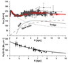 |
Fig. 1. Observed and modelled radial and vertical force field profiles as functions of Galactocentric distances. Top: rotation curve of the Galaxy. The observed rotation curve is represented by the points with error bars, which indicate masers data from high-mass star-forming regions (Reid et al. 2019; Rastorguev et al. 2017), and H I and CO tangent-point data (Burton & Gordon 1978; Clemens 1985; Fich et al. 1989). The red curve shows the analytical rotation curve expressed by Eq. (10). The contributions of the modelled disc (continuous curve), bulge (short-dashed line), and dark halo (long-dashed line) to the axisymmetric Galactic potential are also shown. Bottom: vertical force, Kz, at z = 1.1 kpc as a function of the Galactic radius. The black dots with error bars are from observation measurements by Bovy & Rix (2013), while the solid grey curve shows the Kz force radial profile at z = 1.1 kpc resulting from our Galactic model. |
Physical and structural parameters of the disc components of the axisymmetric Galactic model.
Physical and structural parameters of the spheroidal components of the Galactic model.
The stellar orbits were calculated through the numerical integrations of the equations of motion, defined by the Hamiltonian function, given as
![Mathematical equation: $$ \begin{aligned} H(R,p_r,z,V_z)=\frac{1}{2}\left[p_r^2+\frac{L_z^2}{R^2}+V_z^2\right]+\Phi _0(R,z), \end{aligned} $$](/articles/aa/full_html/2023/12/aa47223-23/aa47223-23-eq13.gif) (12)
(12)
where pr and Vz are the linear radial momentum and vertical velocity, respectively, and Lz is the angular momentum, which is a constant in the axisymmetric approximation (all momenta are given per mass unit).
3. 3D stellar dynamics on the representative plane
The dynamical model defined by the Hamiltonian in Eq. (12) has two degrees of freedom. The resulting stellar motion can be formally represented by two coupled oscillations: one, in the radial (equatorial) direction, is described by the pair of variables R–pr, and the other, in the vertical direction, is described by the pair z–Vz. The phase space of the system is four-dimensional, which makes it difficult to visualise the stellar orbits; however, in this paper we introduce a representative plane that allows us to present the main features of the 3D stellar dynamics. This plane is the R–Vφ plane, where Vφ is the tangential velocity defined as Vφ = Lz/R; we show this plane in Fig. 2.
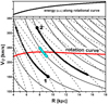 |
Fig. 2. Topology of the Hamiltonian (Eq. (12)) on the representative R–Vφ plane. The continuous curves are the levels of the angular momentum Lz = R × Vφ, while the dashed curves are the energy levels, calculated with the fixed initial values pR = 0, z = 0 and Vz = 20 km s−1. The rotation curve is shown by red dots. The projections of the three 3D orbits on the plane are: the Sun’s orbit (cyan dots), one orbit starting at configuration 1, and another at configuration 2 (black dots). The motion always occurs along a fixed Lz-value due to conservation of the angular momentum, Lz. The conservation of the energy during the motion defines two turning points of each orbit, both lying at the intersections of the corresponding Lz- and energy levels. Top panel: the total energy (see Eq. (12)), in arbitrary units, calculated along the rotation curve, as a function of R. |
To study the stellar motions on the R–Vφ plane, we fixed, in this paper, the initial values of the planar linear momentum at pr = 0 and the vertical height at z = 0. It is worth noting that this choice preserves the generality of the presentation, since all closed stellar motions under the potential given by Eq. (11) pass through these conditions. The initial value of the vertical velocity was chosen as Vz = 20 km s−1, except when the dependence of the motion on the initial vertical configuration was analysed (Sect. 5). The chosen velocity value is close to the value of the standard deviation of the Vz distribution of the stars from Gaia Data Release 3 (Prusti 2016; Vallenari 2023), with |z|< 1 pc (we obtained σVz = 18 km s−1).
First, we plot on the R–Vφ plane in Fig. 2 the main characteristics of the Hamiltonian dynamics: the orbital energy and the angular momentum, which are both constants of motion in our model. The energy levels and Lz-levels are shown by dashed and continuous lines, respectively. The rotation curve obtained using Eq. (10) is shown by the red curve.
By definition, the rotation curve is a place of circular orbits, which are orbits of the minimal energy for a given Lz-value. The geometric interpretation of this condition is that, given the location of a circular orbit on the rotation curve, the corresponding Lz-level is tangent to the minimal energy level on the R–Vφ plane. This fact can be observed in Fig. 2, considering that the energy is continuously increasing with increasing radial distances, R, as shown in the top panel in Fig. 2. The same Lz-level always intersects the levels of higher energy at two points, which are the turning points of the radial oscillations at the condition pr = 0.
We plot in Fig. 2 the direct projections of three 3D stellar orbits: one is the Sun’s orbit (cyan dots), calculated with the initial values R = 8.122 kpc, pr = −12.9 km s−1, Vφ = 245.6 km s−1, z = 0.015 kpc, and Vz = 7.78 km s−1 (Drimmel & Poggio 2018). The orbits of two other fictitious stars (black dots) start at points 1 and 2, respectively, with pr = 0, z = 0, and Vz = 20 km s−1. We can verify that all the orbits are closed, that is, each one evolves between two turning points that belong to the same energy levels, along the corresponding Lz-levels (constant of motion) around the circular orbits, which lie at the intersection of the corresponding energy and Lz-levels.
A detailed analysis of the main features of the stellar motions on the representative R–Vφ plane can be done in two steps: first, by focusing on the radial oscillations on the Galactic equatorial plane, and then on the vertical oscillations around the equatorial plane. By understanding the behaviour of each component of the stellar motion in the axisymmetric potential, we can consider new effects produced by their interaction. We shall do this in the following sections.
3.1. Radial oscillations
The R–Vφ plane shown in Fig. 2 is commonly used for understanding the radial (or planar) motion of stars. Indeed, due to the conservation of angular momentum during the motion, the projections of the 3D orbits are aligned along the corresponding Lz-levels (continuous lines), as observed in the case of our three examples. Since the orbital energy is also conserved in our problem, the orbit’s projections must match the corresponding energy level at conditions pr = 0, which was chosen in the construction of the plane. By definition, this condition defines two turning points of a closed orbit that delimit the path of the radial oscillation on the R–Vφ plane and, consequently, the maximal (Rmax) and minimal (Rmin) values of the radial orbital variation (and the tangential velocity, Vφ, for a given Lz-value).
Any Lz-level crosses the rotation curve (red curve) at one point at Rc on the R–Vφ plane in Fig. 2, which corresponds to the circular orbit of the minimal energy for the corresponding Lz. Under this condition, two turning points merge at one point, characterising the circular orbit with the zero-amplitude R-oscillation, that is, the periodic orbit of the two-degrees-of-freedom problem. All other orbits calculated along the same Lz-level are quasi-periodic orbits oscillating with non-zero R-amplitudes in such a way that the larger the deviations from the rotation curve are, the larger the amplitudes of the radial variations are.
The amplitude of the radial oscillation is related to the planar eccentricity of the orbit as
which is uniquely defined by the values of the orbital energy and angular momentum of the stellar orbit. In the conservative problem considered in this paper, it is a constant of motion. The gain or loss of orbital energy due to some external physical processes, without changing the angular momentum of the system, will increase or decrease the amplitude of R-oscillation and, consequently, the planar eccentricity. This effect, known as “heating” in stellar dynamics, is analogous to the tidal gravitational interactions in planet-satellite systems.
The equatorial motions of the stars are shown in Fig. 3, where we plot the orbits in the subspace R–pR. The orbits were calculated through numerical integrations of the equations of motion defined by the Hamiltonian (Eq. (12)), with initial conditions chosen along the level Lz = 1995 kpc km s−1, which corresponds to the Sun’s orbit (see Fig. 2). To obtain the projection of the 3D motion on the Galactic plane, we gathered the orbital coordinates at the instants when the orbits cross the equatorial plane (the condition z = 0) in the direction of the positive z values (the condition Vz > 0). This approach is known as the Poincaré surface of section method, and allows us to plot the radial motion separately from the vertical one.
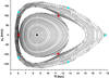 |
Fig. 3. Poincaré map of the stellar 3D orbits calculated with the initial conditions chosen along the Sun’s Lz-level. The initial vertical conditions were chosen at z = 0 and Vz = 20 km s−1. The projections are calculated at instants when the star crosses the equatorial plane with Vz > 0. The orbits are concentric, with the circular orbit at the centre (black dot). This orbit lies at the intersection of the rotation curve and the Sun’s Lz-level on the R–Vφ plane, at Rc = 8.522 kpc and Vφ = 234 km s−1. Red and cyan dots show the projections of two periodic orbits on the Poincaré map corresponding to the 2/1 and 4/1 resonances, respectively (see later Fig. 7). |
Figure 3 shows that all orbits in the R–pR subspace oscillate around a circular periodic orbit (black dot) that lies at the intersection of the corresponding Lz-level and the rotation curve, at Rc = 8.522 kpc and Vφ = 234 km s−1 on the R–Vφ plane in Fig. 2. This periodic orbit appears as a fixed point on the R–pR plane, indicating that the amplitude of the radial oscillation is zero (or e = 0). At the same time, the vertical motion started with the initial Vz = 20 km s−1 has non-zero amplitude; it is a simple oscillation around the equatorial plane (z = 0).
In the vicinity of the fixed point (black dot) between 7.0 kpc and 10.5 kpc, the concentric low-eccentricity orbits with e < 0.2 evolve in good agreement with the epicyclic approximation (e.g. Binney & Tremaine 2008). The orbit of the Sun, with an eccentricity of 0.061, is located in this region of the phase space. The values of the radial and vertical frequencies for the Sun’s Lz level, derived under the epicyclic approximation, are equal to 0.00542 and 0.01387 (in units of 1/Myr), respectively, which corresponds to the radial and vertical periods of 184.5 Myr and 72.07 Myr. These periods derived from the power spectrum of the Sun’s orbit, calculated numerically through our model, are of 161.3 Myr and 75.2 Myr, respectively.
The orbits with increasing eccentricity, however, deviate from the epicyclic approximation and, when the eccentricity approaches 0.5, a notable feature appears in Fig. 3. Indeed, at radial distances beyond 12 kpc we can clearly observe a lack of circulating orbits, but there are some islands on the Poincaré map. As shown below, the orbits in this region are different structurally from the low-eccentricity orbits and are related to the new kind of motion mode. The planar axisymmetric model is not able to explain this feature, and thus we proceed with investigating the vertical motion and its interaction with the planar component.
3.2. The vertical oscillations
The same representative R–Vφ plane shown in Fig. 2 can be used to study the stellar motion in the vertical direction. For this, we plot in Fig. 4, by continuous lines, the levels of the maximal altitude over the equatorial plane that a star reaches during its vertical oscillation (zmax). To obtain zmax, we integrated numerically, over several billion years, the equations of motion defined by the Hamiltonian (Eq. (12)), over the 200 × 200 grid of the initial conditions covering the R–Vφ plane. All orbits started with pR = 0 on the galactic equatorial plane (at z = 0) and with the same initial vertical velocity, Vz = 20 km s−1. The panel at the top of Fig. 4 shows zmax obtained in this way for the circular orbits located along the rotation curve (red curve). We plot also the projection of the Sun’s orbit (cyan dots) along the Lz-level (dashed line) on the R–Vφ plane.
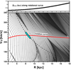 |
Fig. 4. Representative R–Vφ plane shown in Fig. 2, with the same rotation curve (red dots) and the Sun’s orbit (cyan dots) along the Lz-level (dashed line). The equidistant levels are used to represent the amplitude of the vertical oscillation of the stellar orbits (see top panel to associate the absolute zmax-values), with the initial conditions z = 0 and Vz = 20 km s−1. Top panel: the amplitude of the vertical oscillation, zmax, calculated along the rotation curve, as a function of R. |
To understand the zmax–evolution on the Galactic R–Vφ–plane, we considered first the nearly circular orbits, distributed along the rotation curve. For these low-eccentricity orbits, the amplitude of the vertical oscillation increases smoothly with the growing Galactocentric distance, as shown in the top panel in Fig. 4. This result is consistent with the radially decaying exponential mass distribution model applied and is in agreement with the observed increase in the scale height with the increase in the Galactic radius of the disc stars, which is the so-called flaring of the Galactic disc (López-Corredoira et al. 2002; Amôres et al. 2017; Robin et al. 2022).
However, the continuous evolution of the zmax-levels is interrupted in the regions of increasing planar eccentricities when we move away from the rotation curve on the R–Vφ plane in Fig. 4, in the direction of both the higher and lower tangential velocities. To understand this behaviour, it is worth noting that, in domains of regular oscillations, small changes in the initial conditions lead to small changes in the elements of the orbits, in particular, the amplitude, zmax. Consequently, the levels suffer slight displacements on the map when the initial conditions are gradually changed. However, in the vicinity of the resonances, small changes in the initial configurations produce large changes in the orbital elements, which form singular structures, such as resonant islands and stochastic layers. On the dynamical map in Fig. 4, these structures appear in the form of stalactites of different widths.
On the Poincaré map in Fig. 5, the same structures appear as chains of islands contrasting with the orbits, which regularly circulate around the origin. To construct this map, we picked up the orbital coordinates z and Vz at the instants when the star is in the turning point of its orbit (pr = 0) of minimal radial distance (ṗr > 0). The initial configurations of the orbits were chosen along the Sun’s Lz-level and z and Vz fixed at 0 and 20 km s−1, respectively, as in Fig. 3. However, in this case, the initial R-values were extended to very large radial distances, up to 27 kpc.
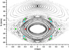 |
Fig. 5. Same as in Fig. 3, except the projections were calculated at conditions pR = 0 and ṗR > 0 on the z–Vz plane. Red, cyan, and green dots show the projections of three periodic orbits on the Poincaré map corresponding to the 2/1, 4/1, and 6/1 resonances, respectively. The large island of orbits oscillating around the centre at z = 0 kpc and Vz = 103.0 km s−1 (black dot) is related to the strong 1/1 resonance (see later Fig. 7). |
Comparing this map to the map of equatorial motion shown in Fig. 3, we verify that the behaviour in the vertical direction is more complicated. We can observe projections of qualitatively different types: there are circulating orbits of regular motion at smaller stellar altitudes. With the increasing height, chains of islands of different widths appear, separated by the stochastic layers. A large island dominates the region of high vertical velocities in the positive half-plane of the map and is surrounded by a sea of chaotic motion. To identify the cause of this behaviour, we applied a special spectral analysis method, the results of which we describe in the next section.
4. The e–z resonances
To understand the features of the resonant motion, we started plotting the amplitude of the vertical oscillation, (zmax), as a function of the initial radial distance, R, on the top panel in Fig. 6. In contrast to the other one shown in the top panel in Fig. 4, the amplitude, zmax, was now calculated with initial conditions chosen along the Lz-level corresponding to the Sun’s orbit. In this case, all orbits are eccentric, with the exception of one located at Rc = 8.522 kpc, at the intersection of the Lz-level with the rotation curve in Fig. 4.
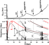 |
Fig. 6. Evolution of the zmax and the radial and vertical frequencies along the Sun’s Lz-level. Top: amplitude of the vertical oscillation of stars as a function of the initial Galactocentric distance. The initial values of Vφ are chosen along the Sun’s Lz-level, while z = 0 and VZ = 20 km s−1. Bottom: dynamical spectrum of the stellar orbits calculated along the Sun’s Lz-level. The nominal positions of some resonances are shown by vertical dashed lines. |
For the orbits starting along the same Lz-level, at the same initial configurations in the vertical direction (z = 0 and Vz = 20 km s−1), the minimal value of zmax is associated with the circular orbit, at Rc = 8.522 kpc. The vertical amplitude generally increases when the orbital eccentricity increases, with both increasing and decreasing in distance from the circular orbit. However, this evolution of zmax is not monotonous, but rather shows sudden increases and decreases at some radial distances. The nature of this behaviour can be analysed using the dynamical power spectrum method, which allows us to detect the change of a regime of motion through the analysis of the evolution of the main frequencies of the dynamical system (a detailed description of the method and its applications to different systems is found in e.g. Michtchenko et al. 2002, 2017).
The bottom panel of Fig. 6 shows two proper frequencies, fr and fz, which are the frequencies of the radial and vertical oscillations, respectively, as functions of the radial distance, R. The evolution of the fr-frequency (red dots) and its harmonics is monotonous over the whole R-range; it reaches the maximal value at Rc = 8.522 kpc, which is expected since the circular orbit is an equilibrium solution of the effective potential,  , with the constant Lz. On the other hand, the behaviour of the fz-frequency (black dots) on the dynamical spectrum is highly non-harmonic and we can observe the appearance of bifurcations, stable islands, and an erratic scattering of the dots, which is characteristic of the chaotic motion.
By analysing the evolution of the proper frequencies in the bottom panel of Fig. 6 we verified that bifurcations occur when beats between two independent frequencies occur. This condition is known as resonances between distinct modes of motion, and leads to changes in the regime of motion. One beat occurs around R = 14 kpc, where fR ≅ 2 fz, giving rise to the island of the 2/1 resonant motion. The periodic orbit of the 2/1 resonance is shown in the subspaces R–pR (top) and z–Vz (bottom) in Fig. 7 (Col. a); the projections of this orbit in the Poincaré maps are shown by red dots in Figs. 3 and 5.
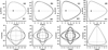 |
Fig. 7. Resonant periodic orbits on the R–pR plane (top row) and z–Vz plane (bottom row). The initial conditions were chosen along the Sun’s Lz-level, while z = 0 and Vz = 20 km s−1. Column a: The 2/1 resonant orbit with e = 0.45 (red dots on the Poincaré maps in Figs. 3 and 5). Column b: The 4/1 resonant orbit with e = 0.72 (cyan dots in Figs. 3 and 5). Column c: The 6/1 resonant orbit with e = 1.01 (green dots in Fig. 5). Column d: The 1/1 resonant orbit with e = 0.802 (black dot in Fig. 5). |
The beating frequencies are also observed at R = 17.8 kpc in the dynamical spectrum at the bottom of Fig. 6 this event is associated with the 4/1 resonance. The radial and vertical oscillation modes of the corresponding periodic orbit are shown in Fig. 7 (Col. b); the projection of this orbit in the Poincaré maps is shown by cyan dots in Figs. 3 and 5. In Fig. 5, we also show, by way of green dots, the projection of the 6/1 resonant orbit (see Fig. 7c); the location of this resonance in the dynamical spectrum is shown at R = 19.2 kpc.
We denote these resonances as the e–z resonances, where e and z denote planar eccentricities and vertical heights of stellar orbits, respectively. The most important of the e–z resonances is the 1/1 resonance, the domain of which is large and separated by the layers of chaotic motion (separatrices). For a given value of Lz, it appears at very large Galactic distances; in the dynamical map in Fig. 6, its domain extends from 20 kpc to 35 kpc. The motion inside the 1/1 resonance is stable, with the amplitude of the vertical oscillation reaching its minimal value at the centre (locus) of the resonance at ∼27 kpc; this locus appears as a fixed point (black dot) in the Poincaré map in Fig. 5. The locus is a periodic orbit of the 1/1 resonance shown in Fig. 7 (Col. d). The neighbourhood of the 1/1 resonance is generally a domain of highly unstable motion. This is due to the overlap of the high-order resonances of the type fr/fz ≅ m/n (m and n are integers).
Finally, it is worth emphasising that, comparing the evolution of the two frequencies at the bottom of Fig. 6 we note the following qualitative difference in the behaviour of the two independent modes: while the radial motion seems to be unaffected by the passage through the resonances, their impact on the vertical motion is significant. This could be explained by the peculiar characteristics of the massive disc potential.
5. The dependence on the initial vertical velocity, Vz
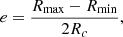
In this section, we investigate the resonant behaviour as a function of the initial vertical velocity, Vz. For this, we introduce the representative plane, R–Vz, of the initial conditions and fix the rest of the variables at pr = 0, z = 0 and Lz = 1995 kpc km s−1, the latter corresponding to the Sun’s angular momentum.
Figure 8 presents the amplitude of the vertical oscillation in the form of the zmax-levels on the representative R–Vz plane. The red curve shows the positions of the circular orbits of the constant Lz, which are slightly dislocated in the direction of the larger Galactocentric distances, when the initial vertical velocities increase. The panel beside the R–Vz plane allows us to quantify the zmax-amplitude, showing its values calculated along the loci of the circular orbits (red curve). The smoothed evolution of this quantity with the increasing initial Vz can be observed.
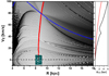 |
Fig. 8. R–Vz plane of initial conditions chosen along the Sun’s Lz-level, with pR = 0 and z = 0. The equidistant levels of the maximal vertical deviation from the equatorial plane, zmax, are shown by continuous curves; its value mainly increases with the increasing Vz (see beside panel to associate the absolute zmax-values). The red curve shows the location of the circular orbits with Lz = 1995 kpc km s−1 as a function of the initial Vz. The structures, which are characteristic of the e–z resonances, appear on both sides of the red curve, expanding their domains with increasing eccentricities. The blue curve shows loci of the very strong 1/1 resonance. The projection of the Sun’s orbit is shown by cyan dots; its maximal z-amplitude is around 0.85 kpc. Side panel: zmax-values as a function of the initial Vz, for circular orbits (red curve) and orbits with initial R = 13 kpc (black curve). |
The bifurcation structures, which are characteristic of the resonances, appear outside the loci of the circular orbits in Fig. 8 and are strengthened with the increasing planar eccentricities of the orbits. The black curve on the side panel shows the evolution of the zmax-amplitude calculated along the constant initial R = 13 kpc. We can observe behaviour similar to that shown in the top panel in Fig. 6, indicating the passages through some e–z resonances. The most prominent passage is through the 1/1 resonance, the loci of which are shown by the blue dots in Fig. 8. The projection of the Sun’s trajectory on the R–Vz plane is shown by cyan dots. Its proximity to the rotation curve prevents it from being captured in one of the resonances.
6. Conclusions
In this paper, we report the existence of resonant motion of the kind e–z (e and z being the planar eccentricity and vertical altitude of stellar orbits, respectively), produced by the axisymmetric Galactic 3D potential.
We investigated the spatial motion of the stars by applying an elaborated model of the axisymmetric potential of the Galactic disc (Barros et al. 2016). The model accounts for the combined gravitational effects due to the two stellar discs (thin and thick discs) and two gaseous discs (H I and H2 discs). Moreover, to account for a radially exponential Galactic mass distribution, each of the discs is approximated by the composition of the three MN disc profiles (Smith et al. 2015). The physical and structural parameters of the modelled components were chosen to correspond to the observable rotation curve of the Galaxy.
The motion of stars in the axisymmetric Galactic potential was investigated in the whole phase space by applying several techniques from celestial mechanics. One of those is the dynamical mapping of the representative plane chosen here as the R–Vφ plane. Based on the conservation laws, we identify two independent modes of stellar motion, radial and vertical ones. The radial motion is an oscillation around the circular solution, which is a circular orbit belonging to the rotation curve and characterised by the same angular momentum as the radial mode. The vertical motion is an oscillation around the equatorial Galactic plane.
For nearly circular orbits, with small planar eccentricities, two oscillations are weakly coupled. It is worth noting that the circular orbits survive even when vertical velocities are very high. However, when the planar eccentricities increase, the coupling between two modes of motion also increases. Their interaction is better visualised in the dynamical power spectra, which clearly show the regions in the phase space where two proper frequencies are commensurate. These beating frequencies indicate the resonant zones, which we denote as e–z resonances.
In Hamiltonian theories, resonances are fundamental properties of dynamical systems with two or more degrees of freedom. They occur in domains of the phase space where the frequencies of the independent modes of motion are commensurate. The locations and the sizes of the resonant domains are strongly dependent upon the physical parameters of the model adopted to describe the system under study. Thus, by associating some observable structures of the objects with the resonances, we can assess the reliable ranges of the parameters of the applied model. One example of this approach is shown in Michtchenko et al. (2018), in which we relate the moving groups in the solar neighbourhood to the Lindblad resonances produced by the spiral perturbations, and estimate the spiral strength and pattern speed.
The main features of the e–z resonant motion are a sudden increase or decrease in the amplitude of the vertical oscillation, the capture and entrapment of stars inside the stable resonant zones, enhancing the density of those zones, and the depletion of the regions close to the separatrices of the resonances. This behaviour is characteristic of the vertical oscillations, while the planar radial motion is only slightly affected by the e–z resonances; this is probably due to the peculiar properties of the disc potential.
It is worth emphasising that, despite the fact that the resonances occur at very large Galactic distances, the high eccentricities of the resonant orbits enable us to detect them in the solar neighbourhood, according to Fig. 7. Indeed, analysing the behaviour of one thousand randomly chosen stars in the Gaia Data Release 3 sample from the solar vicinity (R⊙ ± 0.2 kpc and |pR|≥100 km s−1), we detected resonant oscillations in 10% of the objects, mainly inside the 2/1 resonance. Of course, whether these stars are really evolving inside the e–z resonances depends strongly upon the parameters adopted in our model. Thus, we should be able to observe the described manifestations of the e–z resonances by analysing the distribution of the observable proper elements of the stars. The comparison to theoretical predictions could allow us to improve unknown values of the parameters that describe the observable Galactic mass distribution.
Acknowledgments
We acknowledge the anonymous referee for the detailed review and for the many helpful suggestions which allowed us to improve the manuscript. This work was supported by the Brazilian agencies Conselho Nacional de Desenvolvimento Científico e Tecnológico (CNPq), and São Paulo Research Foundation (FAPESP). This work has made use of the facilities of the Laboratory of Astroinformatics (IAG/USP, NAT/Unicsul), funded by FAPESP (grant 2009/54006-4) and INCT-A. This work has made use of data from the European Space Agency (ESA) mission Gaia (https://www.cosmos.esa.int/gaia), processed by the Gaia Data Processing and Analysis Consortium (DPAC, https://www.cosmos.esa.int/web/gaia/dpac/consortium). Funding for the DPAC has been provided by national institutions, in particular the institutions participating in the Gaia Multilateral Agreement.
References
- Amôres, E. B., Robin, A. C., & Reylé, C. 2017, A&A, 602, A67 [NASA ADS] [CrossRef] [EDP Sciences] [Google Scholar]
- Antoja, T., Helmi, A., Romero-Gómez, M., et al. 2018, Nature, 561, 360 [Google Scholar]
- Barros, D. A., Lépine, J. R. D., & Dias, W. S. 2016, A&A, 593, A108 [NASA ADS] [CrossRef] [EDP Sciences] [Google Scholar]
- Barros, D. A., Pérez-Villegas, A., Lépine, J. R. D., Michtchenko, T. A., & Vieira, R. S. S. 2020, ApJ, 888, 75 [NASA ADS] [CrossRef] [Google Scholar]
- Barros, D. A., Pérez-Villegas, A., Michtchenko, T. A., & Lépine, J. R. D. 2021, Front. Astron. Space Sci., 8, 48 [NASA ADS] [CrossRef] [Google Scholar]
- Binney, J., & Schönrich, R. 2018, MNRAS, 481, 1501 [Google Scholar]
- Binney, J., & Tremaine, S. 2008, Galactic Dynamics: Second Edition (Princeton University Press) [Google Scholar]
- Bland-Hawthorn, J., Sharma, S., Tepper-Garcia, T., et al. 2019, MNRAS, 486, 1167 [NASA ADS] [CrossRef] [Google Scholar]
- Bovy, J., & Rix, H.-W. 2013, ApJ, 779, 115 [Google Scholar]
- Burton, W. B., & Gordon, M. A. 1978, A&A, 63, 7 [NASA ADS] [Google Scholar]
- Carlin, J. L., DeLaunay, J., Newberg, H. J., et al. 2013, ApJ, 777, L5 [Google Scholar]
- Clemens, D. P. 1985, ApJ, 295, 422 [NASA ADS] [CrossRef] [Google Scholar]
- Darling, K., & Widrow, L. M. 2019, MNRAS, 484, 1050 [CrossRef] [Google Scholar]
- Drimmel, R., & Poggio, E. 2018, Res. Notes Am. Astron. Soc., 2, 210 [Google Scholar]
- Faure, C., Siebert, A., & Famaey, B. 2014, MNRAS, 440, 2564 [CrossRef] [Google Scholar]
- Feldmann, R., & Spolyar, D. 2015, MNRAS, 446, 1000 [NASA ADS] [CrossRef] [Google Scholar]
- Fich, M., Blitz, L., & Stark, A. A. 1989, ApJ, 342, 272 [NASA ADS] [CrossRef] [Google Scholar]
- Fragkoudi, F., Katz, D., Trick, W., et al. 2019, MNRAS, 488, 3324 [NASA ADS] [Google Scholar]
- Gaia Collaboration (Prusti, T., et al.) 2016, A&A, 595, A1 [NASA ADS] [CrossRef] [EDP Sciences] [Google Scholar]
- Gaia Collaboration (Katz, D., et al.) 2018, A&A, 616, A11 [NASA ADS] [CrossRef] [EDP Sciences] [Google Scholar]
- Gaia Collaboration (Vallenari, A., et al.) 2023, A&A, 674, A1 [NASA ADS] [CrossRef] [EDP Sciences] [Google Scholar]
- Ghosh, S., Debattista, V. P., & Khachaturyants, T. 2022, MNRAS, 511, 784 [CrossRef] [Google Scholar]
- Gómez, F. A., Minchev, I., O’Shea, B. W., et al. 2013, MNRAS, 429, 159 [Google Scholar]
- GRAVITY Collaboration (Abuter, R., et al.) 2018, A&A, 615, L15 [NASA ADS] [CrossRef] [EDP Sciences] [Google Scholar]
- Hernquist, L. 1990, ApJ, 356, 359 [Google Scholar]
- Hunt, J. A. S., Hong, J., Bovy, J., Kawata, D., & Grand, R. J. J. 2018, MNRAS, 481, 3794 [NASA ADS] [CrossRef] [Google Scholar]
- Hunt, J. A. S., Price-Whelan, A. M., Johnston, K. V., & Darragh-Ford, E. 2022, MNRAS, 516, L7 [NASA ADS] [CrossRef] [Google Scholar]
- Kawata, D., Baba, J., Ciucǎ, I., et al. 2018, MNRAS, 479, L108 [Google Scholar]
- Khachaturyants, T., Debattista, V. P., Ghosh, S., Beraldo e Silva, L., & Daniel, K. J. 2022, MNRAS, 517, L55 [CrossRef] [Google Scholar]
- Khanna, S., Sharma, S., Tepper-Garcia, T., et al. 2019, MNRAS, 489, 4962 [Google Scholar]
- Khoperskov, S., Di Matteo, P., Gerhard, O., et al. 2019, A&A, 622, L6 [NASA ADS] [CrossRef] [EDP Sciences] [Google Scholar]
- Laporte, C. F. P., Minchev, I., Johnston, K. V., & Gómez, F. A. 2019, MNRAS, 485, 3134 [Google Scholar]
- López-Corredoira, M., Cabrera-Lavers, A., Garzón, F., & Hammersley, P. L. 2002, A&A, 394, 883 [NASA ADS] [CrossRef] [EDP Sciences] [Google Scholar]
- Michtchenko, T. A., Lazzaro, D., Ferraz-Mello, S., & Roig, F. 2002, Icarus, 158, 343 [NASA ADS] [CrossRef] [Google Scholar]
- Michtchenko, T. A., Vieira, R. S. S., Barros, D. A., & Lépine, J. R. D. 2017, A&A, 597, A39 [NASA ADS] [CrossRef] [EDP Sciences] [Google Scholar]
- Michtchenko, T. A., Lépine, J. R. D., Pérez-Villegas, A., Vieira, R. S. S., & Barros, D. A. 2018, ApJ, 863, L37 [NASA ADS] [CrossRef] [Google Scholar]
- Michtchenko, T. A., Barros, D. A., Pérez-Villegas, A., & Lépine, J. R. D. 2019, ApJ, 876, 36 [NASA ADS] [CrossRef] [Google Scholar]
- Miyamoto, M., & Nagai, R. 1975, PASJ, 27, 533 [NASA ADS] [Google Scholar]
- Momany, Y., Zaggia, S., Gilmore, G., et al. 2006, A&A, 451, 515 [NASA ADS] [CrossRef] [EDP Sciences] [Google Scholar]
- Monari, G., Famaey, B., & Siebert, A. 2015, MNRAS, 452, 747 [NASA ADS] [CrossRef] [Google Scholar]
- Rastorguev, A. S., Utkin, N. D., Zabolotskikh, M. V., et al. 2017, Astrophys. Bull., 72, 122 [NASA ADS] [CrossRef] [Google Scholar]
- Reid, M. J., Menten, K. M., Brunthaler, A., et al. 2019, ApJ, 885, 131 [Google Scholar]
- Robin, A. C., Bienaymé, O., Salomon, J. B., et al. 2022, A&A, 667, A98 [NASA ADS] [CrossRef] [EDP Sciences] [Google Scholar]
- Smith, R., Flynn, C., Candlish, G. N., Fellhauer, M., & Gibson, B. K. 2015, MNRAS, 448, 2934 [Google Scholar]
- Wang, H.-F., Liu, C., Xu, Y., Wan, J.-C., & Deng, L. 2018, MNRAS, 478, 3367 [NASA ADS] [CrossRef] [Google Scholar]
- Wang, H. F., Huang, Y., Zhang, H. W., et al. 2020, ApJ, 902, 70 [Google Scholar]
- Widrow, L. M., Gardner, S., Yanny, B., Dodelson, S., & Chen, H.-Y. 2012, ApJ, 750, L41 [Google Scholar]
- Williams, M. E. K., Steinmetz, M., Binney, J., et al. 2013, MNRAS, 436, 101 [Google Scholar]
All Tables
Physical and structural parameters of the disc components of the axisymmetric Galactic model.
Physical and structural parameters of the spheroidal components of the Galactic model.
All Figures
|
Fig. 1. Observed and modelled radial and vertical force field profiles as functions of Galactocentric distances. Top: rotation curve of the Galaxy. The observed rotation curve is represented by the points with error bars, which indicate masers data from high-mass star-forming regions (Reid et al. 2019; Rastorguev et al. 2017), and H I and CO tangent-point data (Burton & Gordon 1978; Clemens 1985; Fich et al. 1989). The red curve shows the analytical rotation curve expressed by Eq. (10). The contributions of the modelled disc (continuous curve), bulge (short-dashed line), and dark halo (long-dashed line) to the axisymmetric Galactic potential are also shown. Bottom: vertical force, Kz, at z = 1.1 kpc as a function of the Galactic radius. The black dots with error bars are from observation measurements by Bovy & Rix (2013), while the solid grey curve shows the Kz force radial profile at z = 1.1 kpc resulting from our Galactic model. |
| In the text | |
|
Fig. 2. Topology of the Hamiltonian (Eq. (12)) on the representative R–Vφ plane. The continuous curves are the levels of the angular momentum Lz = R × Vφ, while the dashed curves are the energy levels, calculated with the fixed initial values pR = 0, z = 0 and Vz = 20 km s−1. The rotation curve is shown by red dots. The projections of the three 3D orbits on the plane are: the Sun’s orbit (cyan dots), one orbit starting at configuration 1, and another at configuration 2 (black dots). The motion always occurs along a fixed Lz-value due to conservation of the angular momentum, Lz. The conservation of the energy during the motion defines two turning points of each orbit, both lying at the intersections of the corresponding Lz- and energy levels. Top panel: the total energy (see Eq. (12)), in arbitrary units, calculated along the rotation curve, as a function of R. |
| In the text | |
|
Fig. 3. Poincaré map of the stellar 3D orbits calculated with the initial conditions chosen along the Sun’s Lz-level. The initial vertical conditions were chosen at z = 0 and Vz = 20 km s−1. The projections are calculated at instants when the star crosses the equatorial plane with Vz > 0. The orbits are concentric, with the circular orbit at the centre (black dot). This orbit lies at the intersection of the rotation curve and the Sun’s Lz-level on the R–Vφ plane, at Rc = 8.522 kpc and Vφ = 234 km s−1. Red and cyan dots show the projections of two periodic orbits on the Poincaré map corresponding to the 2/1 and 4/1 resonances, respectively (see later Fig. 7). |
| In the text | |
|
Fig. 4. Representative R–Vφ plane shown in Fig. 2, with the same rotation curve (red dots) and the Sun’s orbit (cyan dots) along the Lz-level (dashed line). The equidistant levels are used to represent the amplitude of the vertical oscillation of the stellar orbits (see top panel to associate the absolute zmax-values), with the initial conditions z = 0 and Vz = 20 km s−1. Top panel: the amplitude of the vertical oscillation, zmax, calculated along the rotation curve, as a function of R. |
| In the text | |
|
Fig. 5. Same as in Fig. 3, except the projections were calculated at conditions pR = 0 and ṗR > 0 on the z–Vz plane. Red, cyan, and green dots show the projections of three periodic orbits on the Poincaré map corresponding to the 2/1, 4/1, and 6/1 resonances, respectively. The large island of orbits oscillating around the centre at z = 0 kpc and Vz = 103.0 km s−1 (black dot) is related to the strong 1/1 resonance (see later Fig. 7). |
| In the text | |
|
Fig. 6. Evolution of the zmax and the radial and vertical frequencies along the Sun’s Lz-level. Top: amplitude of the vertical oscillation of stars as a function of the initial Galactocentric distance. The initial values of Vφ are chosen along the Sun’s Lz-level, while z = 0 and VZ = 20 km s−1. Bottom: dynamical spectrum of the stellar orbits calculated along the Sun’s Lz-level. The nominal positions of some resonances are shown by vertical dashed lines. |
| In the text | |
|
Fig. 7. Resonant periodic orbits on the R–pR plane (top row) and z–Vz plane (bottom row). The initial conditions were chosen along the Sun’s Lz-level, while z = 0 and Vz = 20 km s−1. Column a: The 2/1 resonant orbit with e = 0.45 (red dots on the Poincaré maps in Figs. 3 and 5). Column b: The 4/1 resonant orbit with e = 0.72 (cyan dots in Figs. 3 and 5). Column c: The 6/1 resonant orbit with e = 1.01 (green dots in Fig. 5). Column d: The 1/1 resonant orbit with e = 0.802 (black dot in Fig. 5). |
| In the text | |
|
Fig. 8. R–Vz plane of initial conditions chosen along the Sun’s Lz-level, with pR = 0 and z = 0. The equidistant levels of the maximal vertical deviation from the equatorial plane, zmax, are shown by continuous curves; its value mainly increases with the increasing Vz (see beside panel to associate the absolute zmax-values). The red curve shows the location of the circular orbits with Lz = 1995 kpc km s−1 as a function of the initial Vz. The structures, which are characteristic of the e–z resonances, appear on both sides of the red curve, expanding their domains with increasing eccentricities. The blue curve shows loci of the very strong 1/1 resonance. The projection of the Sun’s orbit is shown by cyan dots; its maximal z-amplitude is around 0.85 kpc. Side panel: zmax-values as a function of the initial Vz, for circular orbits (red curve) and orbits with initial R = 13 kpc (black curve). |
| In the text | |
Current usage metrics show cumulative count of Article Views (full-text article views including HTML views, PDF and ePub downloads, according to the available data) and Abstracts Views on Vision4Press platform.
Data correspond to usage on the plateform after 2015. The current usage metrics is available 48-96 hours after online publication and is updated daily on week days.
Initial download of the metrics may take a while.