| Issue |
A&A
Volume 679, November 2023
|
|
|---|---|---|
| Article Number | A58 | |
| Number of page(s) | 19 | |
| Section | Planets and planetary systems | |
| DOI | https://doi.org/10.1051/0004-6361/202347335 | |
| Published online | 08 November 2023 | |
The first scattered light images of HD 112810, a faint debris disk in the Sco-Cen association
1
Max-Planck-Institut für Astronomie,
Königstuhl 17,
69117
Heidelberg, Germany
e-mail: This email address is being protected from spambots. You need JavaScript enabled to view it.
2
Department of Astronomy, University of Geneva,
Chemin Pegasi 51,
1290
Versoix, Switzerland
3
Université Grenoble Alpes, CNRS, IPAG,
38000
Grenoble, France
4
Aix Marseille Univ, CNRS, CNES, LAM,
Marseille, France
5
INAF-Osservatorio Astronomico di Padova,
Vicolo dell’Osservatorio 5,
35122
Padova, Italy
6
Scottish Universities Physics Alliance, Institute for Astronomy, University of Edinburgh,
Blackford Hill,
Edinburgh
EH9 3HJ, UK
Centre for Exoplanet Science, University of Edinburgh,
Edinburgh
EH9 3HJ, UK
7
Space Telescope Science Institute,
3700 San Martin Drive,
Baltimore, MD
21218, USA
8
Steward Observatory, Department of Astronomy, University of Arizona,
933 N. Cherry Ave,
Tucson, AZ
85721, USA
9
LESIA, Observatoire de Paris, Université PSL, CNRS, Université Paris Cité, Sorbonne Université,
5 place Jules Janssen,
92195
Meudon, France
10
University of Exeter, Astrophysics Group,
Physics Building, Stocker Road,
Exeter
EX4 4QL, UK
11
School of Physics and Astronomy, Monash University,
Vic
3800, Australia
12
Jet Propulsion Laboratory, California Institute of Technology,
Mail Stop 321-100,
4800 Oak Grove Drive,
Pasadena, CA
91109, USA
Received:
3
July
2023
Accepted:
11
September
2023
Abstract
Context. Circumstellar debris disks provide insight into the formation and early evolution of planetary systems. Resolved belts in particular help to locate planetesimals in exosystems, and can hint at the presence of disk-sculpting exoplanets.
Aims. We study the circumstellar environment of HD 112810 (HIP 63439), a mid-F-type star in the Sco-Cen association with a significant infrared excess indicating the presence of a circumstellar debris disk.
Methods. We collected five high-contrast observations of HD 112810 with VLT/SPHERE. We identified a debris disk in scattered light, and found that the debris signature is robust over a number of epochs and a variety of reduction techniques. We modeled the disk, accounting for self-subtraction and assuming that it is optically thin.
Results. We find a single-belt debris disk, with a radius of 118 ± 9 au and an inclination angle of 75.7−1.3+1.1. This is in good agreement with the constraints from spectral energy distribution modeling and from a partially resolved ALMA image of the system. No planets are detected, though planets below the detection limit (~2.6 MJ at a projected separation of 118 au) could be present and could have contributed to sculpting the ring of debris.
Conclusions. HD 112810 adds to the growing inventory of debris disks imaged in scattered light. The disk is faint, but the radius and the inclination of the disk are promising for follow-up studies of the dust properties.
Key words: circumstellar matter / planet-disk interactions / planetary systems / techniques: high angular resolution
© The Authors 2023
 Open Access article, published by EDP Sciences, under the terms of the Creative Commons Attribution License (https://creativecommons.org/licenses/by/4.0), which permits unrestricted use, distribution, and reproduction in any medium, provided the original work is properly cited.
This article is published in open access under the Subscribe to Open model.
Open Access funding provided by Max Planck Society.
1 Introduction
The outer reaches of exoplanet systems remain difficult to study, with only ~100 exoplanets detected beyond ~10 au to date1. Young exoplanet systems are particularly difficult to study since transit and radial velocity surveys are generally less sensitive to planets around young, active stars – only ~5% of planets with known ages are younger than 100Myr. However, understanding the properties of young planets at all spatial scales, and their population statistics, is key to understanding the formation and early evolution of exoplanetary systems.
Circumstellar debris disks provide a unique view of these outer exosystems (for a review see Hughes et al. 2018). While protoplanetary disks are the sites of active ongoing planet formation, slightly older star systems are often surrounded by circumstellar debris disks that are made up of planetesimals and small dust grains in orbit around the star. The small particles are second-generation dust that is generated by collisions of the planetesimals (e.g., Wyatt 2008, and references therein). Detection of these small particles therefore implies that there is a reservoir of planetesimals, and hints at the location of this material. Further, this dust is quickly depleted from the system, so observations of the small dust indicate that these collisions between planetesimals are ongoing: this could imply the presence of unseen planets that stir the disk and enhance the rate of collisions, and such unseen planets would also impact the structure of the disk (e.g. Wyatt et al. 1999; Krivov 2010; Matthews et al. 2014). In many cases, planets would require masses between that of Neptune and Jupiter to explain the level of stirring observed in well-characterized debris disks (Pearce et al. 2022).
The presence of debris disks can be inferred from a spectral energy distribution (SED) in the case that there is significant excess emission in the mid- and far-infrared (IR) relative to the predicted emission of a stellar photosphere alone. If the excess is well characterized, the disk temperature(s) can also be inferred from the SED alone, and with suitable assumptions about the grain properties, corresponding disk location(s) can be derived. Some nearby, bright disks can also be resolved, allowing for detailed study of their morphology. Several debris disks have been resolved in thermal emission since the first such detections with the Infrared Astronomical Satellite (IRAS; Aumann 1985), and in scattered light in the optical and near-IR with high-contrast imaging facilities (Smith & Terrile 1984; Schneider et al. 1999). In the last decade, both scattered light and thermal disk imaging has advanced significantly. The advancement of adaptive optics (AO) and coronagraphic technology has led to many new disks being detected in scattered light optical- and near-IR high-contrast imaging (e.g., Kasper et al. 2015; Currie et al. 2015; Lagrange et al. 2016; Matthews et al. 2017; Bonnefoy et al. 2021); the Atacama Large Millimeter Array (ALMA) has provided an unprecedented look at the thermal emission of disks at millimeter wavelengths (e.g, Boley et al. 2012; MacGregor et al. 2013, 2019; Ricci et al. 2015; Lieman-Sifry et al. 2016). These thermal and scattered light images allow for positions of planetesimal belts and small dust grains in the system to be traced, and also open the opportunity for detailed characterization of the grain properties, such as measuring the scattering phase function of the disk and thereby constraining grain sizes and compositions (e.g., Milli et al. 2017).
This treasure trove of resolved thermal and scattered light images reveals complex structures that cannot be deduced from the SED alone, such as spirals, warps, and gaps between distinct belts of dust (Feldt et al. 2017; Bonnefoy et al. 2017; Marino et al. 2018, 2019; MacGregor et al. 2019). One proposed explanation of such complex disk features is the gravitational influence of unseen planets in the system. More generally, debris disks may provide insight into the bulk compositions of exoplanets since the debris material is generated in collisions of planetesimals, which are also the building blocks for any rocky planets forming at the widest separations.
The Scorpius-Centaurus (Sco-Cen) OB association has been a particularly fruitful location for studies of young circumstellar disks. Many of its debris disks, as well as some protoplanetary and transition disks, have been studied in detail in this region. The association is young, with members spanning ~7–18 Myr (Pecaut & Mamajek 2016), is nearby (~ 110–130 pc), and has a disk fraction of around a third, with no significant variation in the disk fraction between the three subgroups (Chen et al. 2011). As a large association with a relatively narrow age range, the region is particularly valuable since it provides a snapshot of the outer architectures in planetary systems, even among stars with similar masses and formation environments. A number of scattered light debris disk studies with the SPHERE (Spectro-Polarimetric High-contrast Exoplanet REsearch) instrument at the VLT (Very Large Telescope) and GPI (Gemini Planet Imager) at the Gemini telescope have revealed significant diversity of disk architectures among Sco-Cen stars, hinting at the possible presence of many outer planetary systems (e.g., Kalas et al. 2015; Hung et al. 2015; Feldt et al. 2017; Bonnefoy et al. 2017, 2021; Matthews et al. 2017; Engler et al. 2020; Hom et al. 2020).
HD 112810 (HIP 63439) is an F4-type star in the Lower Centaurus Crux (LCC) region of the Sco-Cen association (de Zeeuw et al. 1999; Rizzuto et al. 2011; Gagné et al. 2018), with an age of ~ 17 Myr (Pecaut et al. 2012) and a distance of 133.7 ± 0.3 pc (Gaia Collaboration 2021). The star has a well-characterized IR excess, which has been studied with several facilities including Spitzer (Werner et al. 2004) and WISE (Wright et al. 2010). Chen et al. (2011) detected excess emission at both 24 µm and 70 µm with Spitzer/MIPS, and Chen et al. (2014) subsequently presented Spitzer/IRS spectroscopy of the target. HD 112810 also shows a clear excess in the WISE W3 (11.6 µm) and W4 (22.1 µm) channels (McDonald et al. 2012; Cotten & Song 2016). Chen et al. (2014) used blackbodies to model the Spitzer MIPS and IRS measurements of HD 112810, and found evidence for two distinct temperatures of dust, at  and
and  respectively. This corresponds to radii of ~8 au and ~160 au, following the conversion in Pawellek & Krivov (2015) which modifies the blackbody equilibrium temperature of grains based on realistic compositions, though there is an inherent uncertainty in deriving dust positions from SED information alone. Jang-Condell et al. (2015) modeled the same Spitzer data as presented in Chen et al. (2014) using more realistic grain properties (as opposed to blackbodies), and derived somewhat hotter temperatures of 405 ± 35 K and 69.5 ± 0.9 K, corresponding to physical locations of 0.951 ± 0.2 au and 24.3 ± 2.9 au using the grain property treatment described in Jang-Condell et al. (2015). The LIR/L* value is near the faintest end of the distribution of disks that have been detected in scattered light to date (Esposito et al. 2020, see their Fig. 15).
The HD 112810 debris disk has been detected in the continuum with ALMA (Lieman-Sifry et al. 2016) at a peak signal to noise ratio of 8.6. The disk was resolved along the major but not minor axis, leading the authors to derive a disk inclination >67°, and an outer radius for the dust belt of  au (using the updated Gaia distance to the target). Only relatively edge-on disks are detectable in total intensity scattered light images, for several reasons. For an optically thin disk, the integrated dust quantity along each line of sight is higher for a highly inclined disk, and this corresponds to a higher peak disk flux. Many disks are strongly forward scattering (e.g., Milli et al. 2017), further boosting the peak surface brightness of an edge-on disk relative to a face-on disk. Further, the angular differential imaging technique for high-contrast imaging is biased against detecting axisymmetric signal: in this method, a sequence of observations at different telescope orientations are used to model and subtract the stellar point spread function (PSF) from each image. Such signal is present regardless of the telescope orientation, and is therefore subtracted with the stellar PSF (e.g., Milli et al. 2012). These biases are clearly confirmed in observations: in the sample from Esposito et al. (2020), 15/18 disks detected in total intensity have an inclination ≥80°, and 17/18 have inclination ≥75°.
The ALMA observations of HD 112810, which indicate a relatively large outer dust radius and an inclination of >67°, suggest that a total intensity scattered light detection of the disk may be possible, but is challenging depending on the true inclination of the disk. While the most edge-on disks are the easiest to detect, those at more modest inclinations provide interesting characterization opportunities: in particular, the geometry of these disks is such that the front and back edges are well separated from each other and from the host star in disk images, meaning that the scattering phase function (SPF) of the disk can be measured across almost the full range of scattering angles. This can be key in untangling the grain structure and composition (e.g., Milli et al. 2017). These grains provide a route to understand the bulk compositions of exoplanets, since these dust grains are generated through the collisions of planetesimals. Such planetesimals should trace the compositions of any rocky exoplanets that form at wide separations.
In this paper, we present the first scattered light images of the HD 112810 debris disk, collected with the VLT/SPHERE high-contrast imager. We observed the target as part of two surveys of multi-belt, or “holey” debris disks, selected based on the target SED (Matthews et al. 2018; Bonnefoy et al. 2021, and references therein). The twin goals of these surveys were to search for planets in the debris disk gaps, and to characterize the disks themselves in scattered light. The paper is organized as follows: we first reassess the stellar properties of HD 112810 in Sect. 2. We describe our observations and data reduction in Sects. 3 and 4 respectively. We model the disk structure in Sect. 5 and discuss the constraints on possible planets in the system in Sect. 6. Finally, we discuss key takeaways of this work in Sect. 7.
Observing log for HD 112810.
2 Stellar properties of HD 112810
The characterization of the stellar properties of HD 112810 is based on the methods described in Desidera et al. (2021). HD 112810 is a single star, with no physical companions detected in the HARPS radial velocity monitoring (16 epochs over 671 days, see Sect. 6.3; Grandjean et al. 2023), the Gemini/NICI snapshot survey (Janson et al. 2013) or in the Gaia catalog (where no comoving objects are found up to more than 20 000 au projected separation2). Several indicators in the Gaia data further indicate that unseen stellar companions are unlikely (see Sect. 6.4 for details). Therefore, we can safely adopt the Gaia parameters (DR3) to evaluate the Sco-Cen membership as previously inferred by de Zeeuw et al. (1999), Rizzuto et al. (2011). Using BANYAN Σ3 (Gagné et al. 2018), which compares the Gaia position, parallax, proper motion, and radial velocity of a target to confirmed members of various moving groups, we found a 98.9% membership probability for LCC, 0.9% for UCL and just 0.2% for a field object. Therefore, we assume the membership to LCC and adopt a corresponding age of 17±3 Myr for the system (Pecaut et al. 2012), though we note that future works with Gaia data will likely determine more precise ages for the Sco-Cen subgroups (see e.g., Ratzenböck et al. 2023).
The star is a mid-F-type star with marginally significant reddening. From the observed photometric colors, and adopting E(B-V) = 0.016 ± 0.016 (Montalto et al. 2021, based on the reddening maps from Lallement et al. 2018), we derived Teff = 6637 ± 120 K using Pecaut & Mamajek (2013) tables4. Adopting these values and the Gaia trigonometric parallax, and limiting the fit to the plausible ages for LCC, we used the PARAM web interface5 (da Silva et al. 2006) to derive the stellar mass and radius. The PARAM interface allows for probabilistic fitting of Teff, [Fe/H], parallax, and age to the PARSEC stellar models (Bressan et al. 2012), in order to derive stellar mass and radius. For the case of HD 112810, we used a tight age constraint (17 ± 3 Myr) corresponding to the Sco-Cen membership, and determined a mass of 1.399 ± 0.037 M⊙ and a radius of 1.369 ± 0.032 R⊙ for HD 112810. Note that these uncertainties are model-fitting uncertainties only, and do not include any systematic uncertainties in the PARSEC models. The corresponding stellar luminosity is 3.30 L⊙.
3 Observations
We imaged HD 112810 with the SPHERE high-contrast imager (Beuzit et al. 2019) at the VLT. We collected a total of 6 distinct observing sequences on the target, with four of those being successfully completed; details of each observation are given in Table 1. All of our observations were collected in the IRDIFS mode, whereby light is split through a dichroic mirror, and images are simultaneously recorded in two different wavelength ranges, with the dual-band IR imager IRDIS (Dohlen et al. 2008; Vigan et al. 2010; Zurlo et al. 2014) and the integral field spectrograph (IFS; Claudi et al. 2008; Mesa et al. 2015). To suppress starlight we used the N_ALC_YJH_S coronagraph, which has an inner working angle of ~0.1″. We collected all of the observations in pupil-stabilized mode, whereby the field naturally rotates with respect to the pupil position over the course of the observing sequence. This means that the stellar speckles have a consistent orientation between images, while any circumstellar material appears to move between images as the field rotates. This allows for angular differential imaging (ADI; Marois et al. 2006) to construct reference images of the quasi-static stellar speckles that can then be removed from the science images.
The first series of observations, in 2016, were collected as part of three SPHERE programs, all of which had a primary aim of searching for giant planets in systems with known debris disks (see Matthews et al. 2018; Lombart et al. 2020). These observations all used the dual-band DB_H23 IRDIS filter (λ = 1593 nm, Δλ = 52 nm and λ = 1667 nm, Δλ = 54 nm), and the YJ mode of the IFS (39 wavelength channels between 0.95 and 1.35 µm), to be optimized for sensitivity to exoplanets. Our data processing revealed a very faint scattered light disk in the IRDIS data (see Sect. 4).
After the identification of this disk, we revisited the target with the aim of boosting the signal-to-noise of our detection. We collected two observation sequences on consecutive nights in February 2020. For these observations, we used the broadband B_H filter (λ = 1625 nm, Δλ = 290 nm) in order to collect more disk photons, as well as the same YJ mode of the IFS. We also used an extended integration time and field rotation (see Table 1) to improve the sensitivity relative to the early observations.
For observation (1) only acquistion frames were collected before the observation was aborted; for observation (5) the sequence was aborted after 10th cube (140th image) due to a technical fault. In the final cube before the sequence was aborted, the header value HIERARCH ESO TEL PARANG END is incorrectly listed as 0.000, but accurate parallactic angles can still be derived for each slice based on the telemetric values in the header. Since the weather conditions were good until this technical fault, we include this full sequence of observations in our analysis. The other four observations were all collected in good weather conditions, and the target was always at airmass <1.2; we list the seeing and field rotation of each observation in Table 1.
Each observing sequence included several calibration frames. Specifically, we collected at least one flux calibration frame and one center calibration frame with both IRDIS and IFS for each observation. For the flux frames, the star center was offset from the coronagraph so that the PSF can be accurately measured. For the center frames (also known as waffle frames), two periodic modulations were applied to the deformable mirror such that four satellite spot images were created in a square pattern, equally displaced from the stellar position. This allows the star center position to be reconstructed to an accuracy of ~0.1 pix (1.2mas; Vigan et al. 2016) behind the coronagraph. The flux and center calibration frames were collected immediately before and/or after the science sequence. For some observations, we also collected sky background frames at the end of observation sequence.
4 Data processing
The HD 112810 disk is very faint in scattered light, as can be seen in Fig. 1. We performed data reductions with several independent pipelines and algorithms, to demonstrate the robustness of our detection and ensure that the extracted physical parameters of the disk are not biased by the specific choice of reduction algorithm. We used two ADI based approaches for each dataset, and also used a reference library RDI based approach for the IRDIS DB_H23 data. The disk was recovered in all IRDIS data reductions except for the 2016 Mar 16 epoch, and in none of the IFS data reductions. The data reduction is split into two distinct phases: firstly a pre-cleaning step, where individual frames are cleaned and calibrated, and secondly a speckle removal step where post-processing algorithms are used to model and remove the stellar PSF and speckle noise.
4.1 ADI with GRAPHIC/PCA
We reduced the SPHERE/IRDIS data from scratch using the GRAPHIC pipeline (Hagelberg et al. 2016). The GRAPHIC pipeline uses a unique Fourier analysis approach to perform frame shifts and rotations, which ensures that high-frequency noise is well preserved during these frame shifts. Hagelberg et al. (2016) demonstrate that this technique offers an improved contrast relative to an interpolation method at small separations (≲1″). The pipeline also includes a custom implementation of the commonly used annular Principal Component Analysis (PCA) approach to model and subtract stellar speckles (Amara & Quanz 2012; Soummer et al. 2012).
We briefly describe the key steps here, and refer the reader to Hagelberg et al. (2016) for a complete description of the pipeline. Frames are first registered: during this process key information such as the time and parallactic angle of each frame are extracted from the file header, and the position and extent of the stellar PSF are fitted. A master-sky (where available) or master-dark, and a master-flat are applied to the data. Bad pixels are identified from the dark or sky frames using σ-clipping, and replaced with the median value of neighboring pixels. Frames are re-centered to align with the waffle frame, and the position of the star behind the coronagraph is extracted from the center calibration frames.
We applied ADI with a PCA algorithm to concentric annuli of the image. This allows for the stellar speckles (which have a consistent orientation between images) to be distinguished from any disk or planet signal (which moves between images as the field rotates). When calculating the PCA components to subtract from each frame, we use a minimum separation criterion in parallactic angle that varies with radial separation so as to minimize self-subtraction. Several PCA components are subtracted from each of the images to remove the stellar speckle and leave any disk and planet signal. These subtracted frames are finally derotated to the same on-sky angle, and combined. This process is carried out in a wavelength-by-wavelength fashion, that is, we first apply the PCA to each of the IRDIS H2 and IRDIS H3 filters, and then co-add the images after PCA analysis. Figure 1 (left column) shows the final IRDIS images of the disk, as processed with GRAPHIC/PCA.
We followed a similar data reduction approach for the SPHERE/IFS frames, with a few key differences. We used the vlt-sphere package (Vigan et al. 2015; Vigan 2020) to perform pre-processing, that is, to turn each frame from a 2D image of spectra to a 3D spectral cube. This routine makes use of several esorex functions (Pavlov et al. 2008) and applies dark and flat corrections, calculates the positions of spectra in the 2D image and calibrates their wavelength, and creates an IFU flat. The routine also corrects bad pixels and detector cross-talk (see Vigan et al. 2015 for details). We then applied the GRAPHIC PCA routine as described above. We considered each wavelength separately during the PCA analysis to create a cube of 39 ADI-reduced images. We also co-added the cube of PCA-processed images to create a broadband YJ reduction. We were unable to identify any disk signal in the reduced IFS data, even when all of the wavelengths were stacked and combined. The processed IFS images are shown in Fig. 2.
4.2 ADI with TLOCI and ANDROMEDA
To further rule out the possibility of the disk signal being a reduction artefact, we also reduced the data from scratch at the SPHERE Data Center (DC) by means of the SpeCal pipeline (Delorme et al. 2017; Galicher et al. 2018). For IRDIS data, we applied ADI using the standard Template Locally Optimized Combination of Images (TLOCI) reduction technique (Lafrenière et al. 2007). Similar to the PCA approach, this involves building a custom reference image to subtract stellar speckles from each science observation. The calibration of true north and pixel scale employs observations of compact stellar clusters as described in Maire et al. (2016). These reductions are shown in the middle column of Fig. 1. For the IFS data, we used the ANDROMEDA reduction technique (Cantalloube et al. 2015). This tracks planetary signatures by using a forward-modeling approach and a maximum likelihood estimator (Mugnier et al. 2009). By using the ADI technique and performing pairwise subtraction of the images, the quasi-static stellar halo is removed, while the circumstellar signal rotates through the observation sequence as a function of parallactic angles. The ANDROMEDA reduction of the IFS data is shown in Fig. 2.
The SPHERE DC results for both the IFS and IRDIS support our results with GRAPHIC: the disk is clearly visible in all IRDIS images except for 2016 Mar 16, and is not visible in any IFS reductions. We also searched for additional companions in the IFS field of view. While a number of points with Signal to Noise ratio (S/N) ~ 4 are observed in both the GRAPHIC and ANDROMEDA IFS reductions, these are not consistent between epoch or between reduction method, implying that these are artefacts of the reduction process, as opposed to bona fide companions.
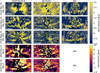 |
Fig. 1 SPHERE/IRDIS images of the HD 112810 debris disk. Each column indicates data processed via a different method: GRAPHIC/PCA (Sect. 4.1; Hagelberg et al. 2016), TLOCI as provided by the SPHERE data center (Sect. 4.2; Delorme et al. 2017) or RDI (Sect. 4.3; Xie et al. 2022); rows indicate each observation epoch. In each case, the two SPHERE/IRDIS channels are co-added. There are no RDI reductions for the BB_H data, since there is far more data collected with the DB_H23 filter in the archive, and the reference library we considered does not collate BB_H data (Xie et al. 2022). The “normalized signal” is calculated relative to the background noise in the wide-field; we note that this is not a true S/N at very small separations, where the noise is higher than the background limit. |
4.3 RDI with reference library and PCA
Different techniques developed to remove the stellar contributions may have different impacts on circumstellar objects, especially extended objects (e.g., debris disks), for which the photometry and the morphology are affected (Milli et al. 2012). To validate the disk detection via GRAPHIC/PCA and DC/TLOCI, we applied reference-star differential imaging (RDI; Smith & Terrile 1984; Golimowski et al. 2006) to recover the scattered light emission of the disk.
We used the reference library implementation from Xie et al. (2022) to construct and subtract reference images; we briefly describe the key steps here and refer the reader to that work for details. In this approach, a library of archival reference star observations are used to create the model of the stellar PSF. We adopted the archived observations of reference stars selected by Xie et al. (2022). The selected master reference library contains 725 SPHERE observations of reference stars in the DB_H23 IRDIS filter. We used the mean square error (MSE) between images to measure the image correlation, and down-selected the 500 most correlated reference images from the master reference library for each science image in each epoch of science observations. For each science observation, we combined the down-selected reference images and formed a single library with non-redundant references. Then we performed PCA on the down-selected reference library to construct the PSF model for each science image in each epoch of HD 112810 observation. For RDI-PCA, we used 400 PCA components to remove the stellar contributions. The temporal images were then derotated and mean combined to form the residual images in H2 and H3. The H2 and H3 bands were processed separately and mean combined to form the final residual image in the H23 band shown in Fig. 1 (right column). The reference library of Xie et al. (2022) does not include BB_H data, since there are many fewer BB_H observations that DB_H23 observations in the SPHERE archive. We therefore only used the RDI approach for the 2016 data, observed in DB_H23.
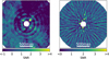 |
Fig. 2 SPHERE/IFS reduced data for HD 112810. Here, we show an image with all data epochs and all wavelengths co-added, with the GRAPHIC/PCA (left) and ANDROMEDA (right) algorithms applied to remove stellar speckles. In both cases, these are S/N maps; for GRAPHIC/PCA each annulus is scaled by the variance in that annulus, causing sharp transitions between concentric annuli. We tried several data reduction approaches and varied the values of tuned parameters. While a few bright spots are seen very close to the inner working angle, these are detected at low significance and are not at consistent locations between epochs – indicating that these are residual stellar speckles. The disk signal is not visible in any IFS data, either in the individual or in the co-added epochs. |
5 Constraints on the disk structure
We modeled the scattered light emission of the HD 112810 disk in order to constrain the disk structure and understand the physical distribution of small dust grains in the disk. In this section we first describe the modeling process, and then detail the various physical models that we tested. We found HD 112810 to be well-fit by a single ring of dust at 118 ± 9 au, that is radially very narrow and vertically unconstrained. We used the epoch (6) observations collected with the IRDIS B_H filter for the modeling, since this is the deepest disk observation and the highest signal-to-noise disk detection. We briefly discuss the best fit for other epochs in Sect. 5.6.
We used the same disk modeling procedure as in Matthews et al. (2017; see also Wahhaj et al. 2014): our process consisted of generating synthetic disk images, subtracting these from the cleaned data, reprocessing that subtracted data, and measuring the goodness of the fit in the reprocessed, residual images. This allows for the modeling to take into account the radially varying transmission of the speckle removal process, as well as any self-subtraction introduced during the speckle removal.
5.1 Synthetic disk model
Our synthetic disk images were generated using the GRaTeR ray tracing code (Augereau et al. 1999, IDL implementation). We modeled the disk as optically thin, meaning that the disk brightness at each point in 3D space is simply defined by the local dust density, the scattering properties of the dust, and the distance of that point from the star.
The generalized form of the disk density in GRaTeR is
![Mathematical equation: $\rho \propto {{\exp \left( {{{\left[ {{{ - \left| z \right|} \over {{\xi _0}}}{{\left( {{r \over {{r_0}}}} \right)}^{ - \beta }}} \right]}^\gamma }} \right)} \over {\sqrt {{{\left( {{r \over {{r_0}}}} \right)}^{ - 2{\alpha _{{\rm{in}}}}}} + {{\left( {{r \over {{r_0}}}} \right)}^{ - 2{\alpha _{{\rm{out}}}}}}} }},$](/articles/aa/full_html/2023/11/aa47335-23/aa47335-23-eq5.png) (1)
(1)
where r and z are the radial and vertical distance from the star, respectively. The vertical structure is parametrized in the exponential term by ξ0, β and γ: ξ0 is the disk vertical scale height at r0, β is the disk flaring index, and γ defines the shape of the vertical profile. For this work, we set β =1 and γ = 2 throughout – that is, a disk with linear flaring and a Gaussian vertical profile.
The radial structure is set in the denominator by a characteristic radius r0 and two power laws defined by αin and αout, characterizing how sharply the dust density decreases with distance from r0. In the case that |αin| = |αout|, the radial maximum dust density is at radius r0. Note that the quoted r0 values and uncertainties refer to the characteristic radius, while the belt width is defined by the αin and αout parameters.
The scattering is parameterized as a function of angle using the Henyey-Greenstein function:
 (2)
(2)
where θ is the scattering angle at each point in the disk and g is the anisotropy parameter, with g = −1 and g = 1 corresponding to the extreme cases of 100% back-scattering and 100% forward-scattering.
The disk flux F at each point in the grid is then derived by combining the local disk density, scattering phase function, and the distance from the star (d2 = r2 + z2) as
 (3)
(3)
Finally, the synthetic disk image is generated by adding the flux terms along the line of sight. For all fits presented in this paper, we used an arbitrary scaling factor of ρ0 when subtracting synthetic disk images from the data.
5.2 Parameter estimation process
Synthetic images were generated following the process described above for each set of physical disk parameters, and were then convolved with a 2D Gaussian to mimic the impact of the telescope PSF. These disk images were subtracted from each slice of the pre-cleaned data cubes (see Sect. 4 for details), at the appropriate rotation angle for that slice. This subtraction of disk images was performed before the application of the stellar speckle removal algorithm. We used the GRAPHIC/PCA (Sect. 4.1) speckle analysis process for model-subtracted cubes, to generate a residual image. This can be a relatively timeintensive procedure, and so we made two changes relative to our original GRAPHIC/PCA reduction described in Sect. 4.1. Firstly, we only performed PCA on the central region of the image, where there is disk flux. We restricted the analysis to a radius of 91 pixels (=1.115″) from the central star. Secondly, we binned temporally to reduce the number of independent images in the datacube. We median-combined each consecutive set of 4 images, accounting for the small parallactic angle changes (always <1°, corresponding to < 1.2 pixel at the disk ansae) between individual images.
This residual image was then used to calculate a χ2 value, as a proxy for the quality of the fit. This χ2 was calculated as  with Fi the data value of the pixel in the residual image, and σr a radially varying uncertainty term, so as to represent the increased stellar speckle noise very close to the star. The σr value is calculated from the standard deviation of pixel values in a small annulus, and inflated to account for the spatial correlation of neighboring pixels. Following Hinkley et al. (2021), we inflated the errors by the square root of the number of pixels in a correlated region, taking into account both the size of the PSF and the radial PSF elongation that derives from the filter bandwidth (which is negligible for the DB_H23 narrowband filters). The inflated uncertainties are calculated as
  , where rpixel(r) represents the uninflated pixel uncertainty, calculated as the standard deviation of pixel values in each annulus.
The χ2 was calculated in a bar-shaped region around the approximate position of the disk. The χ2 value for each synthetic image allows us to assess the relative quality of each fit, and to optimize over disk parameters. We first found a visual fit that appeared to match the observed disk structure, and then performed an MCMC analysis using emcee (Foreman-Mackey et al. 2013), and using the visual fit values as the starting parameters.
5.3 Five parameter fit
We first tested a simple model with five free parameters: three disk parameters (radius r0, forward scattering g, and overall scaling ρ0), and two parameters defining the on-sky position of the disk (inclination itilt and position angle PA). For this fit, we set ξ0 = 4.4 au. This provides an aspect ratio of ~4% at r0 (initially estimated at ~ 110 au), which is the minimum natural aspect ratio of small dust grains in a disk, in the absence of perturbing bodies (Thébault 2009), and we set |αin| = |αout| = 3.5.
We found a good fit to the disk, which is shown in Fig. 3 (top panel), alongside the cleaned data without the disk subtracted, and a residual image (that is, a cleaned datacube with the best-fit model subtracted that is then re-processed with PCA). No significant structure seen in the residuals, indicating that the disk is well-fit with a single dust belt at radius 101 ± 7 au. The best-fitting parameters are listed in Table 2. In Appendix B, we include a corner plot of the posterior, highlighting the key correlations in this dataset. In particular, r0 and itilt are correlated, which is a natural result of the disk geometry: the observable parameter from which the r0 and itilt values are derived is the semi-minor axis of the projected disk ellipse in the SPHERE images, which is equal r0 cos(itilt). A bright patch of emission is seen to the right of the star, which is not co-located with the disk emission; this feature is only seen in one data epoch and is assumed to be an uncorrected stellar speckle.
5.4 The disk vertical profile
To test whether the disk vertical profile can be usefully constrained with the in-hand data, we also performed a fit with one additional free parameter, the disk scale height ξ0, in addition to the five parameters explored in Sect. 5.3. We used a log-uniform prior for ξ0, and used best-fit values from the 5-parameter fit as starting values for all other parameters.
The best fit for this model is shown in Fig. 3 (second row). The posterior for ξ0 traces the prior distribution. The other disk parameters are in good agreement with the values found in Sect. 5.3, except that ρ0 is somewhat higher and less well-constrained, due to the strong anticorrelation between ρ0 and ξ0. A corner plot of the posterior distribution is included in Appendix B.
While formal median and best-fit values are derived from the posterior and quoted in Table 2, we note that these are largely driven by the prior, and in the absence of data constraints a log-uniform prior favors small values. The median and best-fit are lower than the physically motivated natural aspect ratio used in Sect. 5.3; we infer that the vertical structure cannot be constrained, and therefore prefer the physically motivated value of ξ0 = 4.4.
5.5 The disk radial profile
We also explored whether the disk radial profile can be usefully constrained with the available data. In this case we performed a fit with seven free parameters: the five parameters from Sect. 5.3, as well as αin and αout; we fixed the ξ0 = 4.4 as discussed in Sect. 5.4. We used log-uniform priors for both αin and αout.
The best fit for this model is shown in Fig. 3 (bottom row). We find evidence that the disk is narrow: for both α parameters, low values are disfavored. In particular, values of αin ≲ 7.5 are disfavored; above this value the posterior follows the prior. For α0ut, the posterior is moderately well constrained, though very high values are not completely excluded; we find a best-fit value of  . We interpret that the scattered-light disk is narrow – broad disks are ruled out – and that the disk is too narrow to be well-resolved, precluding better constraints on the radial structure to be derived. Effectively, this fit is providing a lower limit on the α parameters, and an upper limit on the disk radial width.
This 7-parameter fit gives a somewhat higher radius than the 5-parameter fit (118 ± 9 au vs 104 ± 7 au). This is a natural result of the disk geometry: while the dust density is at a maximum at r0, the brightness profile is proportional to r/d2, and is therefore at maximum closer to the star than r0 – a broad disk profile characterized by |αin| = |αout| = 3.5 has maximal brightness at 0.91r0, a very narrow disk profile with |αin| = |αout| = 10 has maximal brightness at 0.99r0. The offset between observed maximal brightness and r0 is much smaller for this seven parameter fit with a very narrow disk profile than for the fit presented in Sect. 5.3.
Due to the correlation of r0 and itilt, we also retrieve a somewhat higher inclination value than the 5-parameter fit ( vs.
vs.  ). Both r0 and itilt are ~1.4σ larger for the 7-parameter fit than the 5-parameter fit.
We adopt the results of this 7-parameter fit as the derived disk parameters. The scattered light images of HD 112810 hosts a single, radially narrow ring, with a poorly constrained vertical profile.
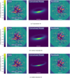 |
Fig. 3 Best fitting models to the data, alongside the raw data and the residual image with the disk subtracted. 3- and 5-σ contours (relative to the background noise) are shown in pink and purple respectively. The three rows show the best fitting models for (a) the 5-parameter fit (b) the vertical structure fit, and (c) the radial structure fit (see Sects. 5.3–5.5). Best-fit parameters are given in Table 2. Residual images are generated by subtracting model disks from the raw data, and then repeating the PCA reduction. The debris disk is well-subtracted in all cases. |
MCMC best fit model parameters for each of the fits described in Sects. 5.3–5.5.
5.6 Disk constraints from other epochs
All the above sections have focused solely on the 2020 Feb 18 data (observation 6 in Table 1), which is the highest significance disk detection due to the long exposure time and broadband filter. We also explored the constraints available from other epochs of data. The 2020 Feb 18 observations are the most constraining: in particular, the radial profile (that is, αin and αout) cannot be well constrained from other epochs of data, which also causes small differences between epochs in the retrieved r0 and itilt as discussed in Sect. 5.5.
6 Limits on substellar companions
Stellar and substellar companions to HD 112810 can be observationally excluded across much of parameter space. As well as the high-contrast imaging observations presented in this work, there are archival radial velocity data, and on-sky acceleration constraints based on the HIPPARCOS and Gaia observations of the systems.
6.1 Observational limits on planets: imaging
To calculate the sensitivity of the SPHERE images, we injected fake companions into the cleaned data cubes, before the processing with the PCA algorithm. We then repeated the full PCA reduction, and measured the brightness of the fake companions in the PCA reduced cubes. This process was repeated a number of times, with fake planets at different position angles and separations. Figure 4 (left) shows the sensitivity of our images in magnitudes relative to the host star. To determine our ability to detect planets in this dataset, we additionally converted these magnitude values to masses. Absolute masses were converted to contrasts using the ATMO isochrones from Phillips et al. (2020) in the relevant SPHERE filters using an age of 17 Myr. The mass sensitivities in the IRDIS bands are given in Fig. 4 (right).
We also converted these limits to completeness curves, using exoDMC (Bonavita 2020), as shown in Fig. 5. exoDMC simulates a suite of test planets, and calculates the fraction of planets that would be observed as a function of mass and separation. For this process, we fixed the inclination of all test planets to the inclination of the disk.
The young age of this system corresponds to an excellent planet sensitivity in the background limited regime, though this regime is limited to ≳150 au due to the distance of the star (133.66 ± 0.29 pc). We are sensitive to planetary mass companions (<13 MJ) beyond ~ 150 mas = 21 au, and to ~2 MJ companions in the background limited regime (beyond ~200 au).
6.2 Imaged candidate companions
Five candidate companions to HD 112810 were identified in Matthews et al. (2018), with separations between 3.5″ and 6.2″ from the host star. In that work, HD 112810 was only observed once, and the candidate companions were deemed to be likely background objects due to their relatively wide projected separations (between 470 au and 830 au). Here, we use the new data from 2020 to reassess the status of these candidate companions, and we confirm that they are indeed background objects (full astrometry and plots are given in Appendix A). We also note that two of these sources are detected in Gaia DR3; the Gaia detections are consistent with the results of the common proper motion test.
We also present astrometry and photometry for one additional candidate companion identified in the 2020 data. This object was too faint to be detected in the 2016 observations (see Fig. 4 for relative sensitivities of the different observations), but is observed in both 2020 epochs. At separation ~5.2″, this candidate is highly likely to be a background object given the local background density, and the wide separation of the companion. Full astrometry for this companion is given in Appendix A.
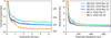 |
Fig. 4 Contrast (left) and mass sensitivities (right) of each epoch of observations. The legend applies to both figures; cool colors indicate the narrowband DB_H23 observations and warm colors indicate the broadband BB_H observations. Companion magnitude limits were converted to mass limits using the ATMO models from Phillips et al. (2020). |
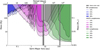 |
Fig. 5 Detection completeness for HD 112810. Shaded rows show completeness for radial velocity observations (blue), HIPPARCOS-Gaia proper motion analysis (pink), and high-contrast imaging observations (green) along with the debris belt positions (gray). Shaded regions indicate the mass vs separation contours at which 10%, 50%, 90% and 99% of companions would be detectable with in-hand data, as described in Sects. 6.3, 6.4 and 6.1 respectively. The inner and outer belt positions are derived from the SED fit and SPHERE modeling respectively. Planetary mass companions and small brown dwarfs at intermediate and wide separations are largely ruled out from the proper motion and imaging constraints. The radial velocity constraints are weaker, ruling out only massive stellar companions at short periods. |
6.3 Observational limits on planets: radial velocities
HD 112810 was observed with HARPS as part of a larger radial velocity survey for massive planets around young stars (Grandjean et al. 2023). That work collected 16 radial velocity points across 8 nights between 2019 Apr 29 and 2021 Feb 28. We independently reduced these data following the process described in Trifonov et al. (2020), and then tested the sensitivity of these data to substellar companions by injecting synthetic companion signals across a range of masses and periods, at the inclination of the debris disk. This process was carried out using an updated version of the code from Barbato et al. (2018).
We found that the radial velocity data for this target are not sufficient to place constraints on substellar companions. This is perhaps unsurprising, given that the host star is a young and early-type star: young stars are typically active, and early-type stars have fewer lines, making this a very challenging host star for radial velocity planet detection. The data are only sensitive to companions ≳200 MJ(=0.19 M⊙) at periods of a few days, and even more massive companions at wider separations (see Fig. 5).
6.4 Observational limits on planets: astrometry
We also examined the constraints available from astrometric analysis of HD 112810, based on the HIPPARCOS and Gaia proper motion measurements: a significant difference in proper motion would indicate that a target is accelerating, due to the presence of an unseen companion. HD 112810 does not show any sign of acceleration: the short-term proper motions of HD 112810 at the Gaia epoch and HIPPARCOS epoch, as well as the long-term average proper motion (calculated from the HIPPARCOS and Gaia position measurements) are all consistent with each other (Brandt 2021). The star has a renormalized unit weight error (RUWE) value of 0.994 (Lindegren et al. 2018; Gaia Collaboration 2023) – strongly implying that the object is a single star. To determine the companion space that is ruled out by these observations, we simulated the observed proper motions for synthetic planets across a range of masses and periods, at the inclination of the debris disk and randomizing over orbital eccentricity, and compared their proper motions to the measured HIPPARCOS, Gaia, and long-term average proper motion. We then calculated the fraction of simulated orbits that are incompatible with the observational constraints. Figure 5 (pink shading) indicates the threshold at which the in-hand data rules out 10%, 50%, 90%, and 99% of all simulated planets. Stellar companions are largely ruled out beyond ~4 au; our detection completeness to brown dwarfs (>13 MJ) is above 50% beyond 3 au based on the proper motion of HD 112810.
6.5 Planet inferences from disk properties
Inferring the presence of planets using the disk structure – either from resolved images or SED constraints – is a method that has long been employed since the discovery of debris disks (see e.g., Mouillet et al. 1997; Quillen 2006). In particular, when two belts are observed with a gap in between, one common hypothesis is that one or more planets may have carved out this gap – in this case, the inferred planet properties can be constrained from the disk structure (see Marino et al. 2018, 2019, 2020; MacGregor et al. 2019, for the most recent applications of this method dedicated to the disks of HD 107146, HD 92945, HD 15115, and HD 206896, respectively). General studies using both analytical arguments and N-body simulations – and exploring the different processes through which planets can carve gaps in disks – allow us to derive the possible number, mass and location of these planets for any given system (e.g., Morrison & Malhotra 2015; Shannon et al. 2016; Yelverton & Kennedy 2018).
The SED of HD 112810 indicates the presence of two belts, located at ~8 au and ~160 au (Chen et al. 2014; Pawellek & Krivov 2015) – somewhat reminiscent of the HR 8799 architecture, which has dust belts at ~15 au and ~145 au (Booth et al. 2016). In the general framework provided by Shannon et al. (2016), if these two rings formed as a single broad belt with a gap carved by planets, that would imply a chain of at least 2 planets, with mass at least 1.8 MJ, close to the planet detection limits of the current work (Fig. 4). However, we note that Shannon et al. (2016) considered only circular planets, and eccentric planets may have a similar gap-carving impact at smaller masses (e.g., Bonnefoy et al. 2017). Further, the properties of the inner debris disk belt are derived from the SED only, and are somewhat uncertain. These very widely spaced belts of debris could also indicate two rings of material that are generated separately, as opposed to a single belt with a gap carved by planets. More detailed disk constraints would be required to make detailed dynamical inferences about planets in the system – in particular, such inferences would benefit from observations with the spatial resolution and sensitivity to resolve the disk radial profile, as well as detect any fainter disk components that are not detected in the current images.
7 Discussion
HD 112810 provides a particularly faint scattered-light disk, barely detectable with present-day facilities: even with several long observations (1–2 h on-sky integration per visit) with a state-of-the-art AO+coronagraph system, the disk is only weakly detected. This is perhaps unsurprising, given its large radius (~118 au), moderate inclination (~75.7°), and the relatively low IR excess of the outer belt (LIR/L* = 5.9 × 10⁻⁴) placing the debris disk at the edge of the population of disks that have been imaged in scattered light (Esposito et al. 2020).
This comparative faintness inevitably makes the disk challenging to study. The disk is nonetheless a valuable addition to the gallery of resolved disks, in particular due to its moderate inclination angle, which traces out a similar geometry as HR4796.
7.1 The GRATER disk model: a single, symmetric ring
In Sect. 5, we demonstrated that the debris disk is well fit as a single ring, with a characteristic radius 118 ± 9 au, a poorly constrained vertical profile, and a very narrow radial profile (see Sect. 5; Fig. 3).
We highlight that some disk parameters are correlated; in particular the radial profile, the characteristic radius r0, and the disk inclination angle. That is, without an accurate determination of the radial profile, the true characteristic radius r0 will be systematically offset from the derived value; this in turn has an impact on the derived inclination angle of the disk. This effect would particularly impact comparative studies where fitted r0 values from various different literature sources are compared, depending on the radial profile assumptions made. Ideally, such comparative works should rederive disk parameters using consistent modeling assumptions.
We do not see any evidence for complex structure in the HD 112810 disk (i.e., multiple rings, gaps, warps, asymmetries etc). However, it is worth noting that this is partly a comment on the relative faintness of the disk. For example, a secondary ring of small grains, such as that observed for HIP 73145 (Feldt et al. 2017) and HIP 67497 (Bonnefoy et al. 2017), would likely be fainter than the main component observed here, and below the noise floor of these observations.
7.2 Comparison of scattered light, thermal emission, and disk SED
Near-IR scattered light images, such as those presented here, trace a different population of grains than those that dominate the ALMA images and SED measurements for the system. We nonetheless briefly comment on how the parameters compare between the SPHERE, ALMA, and SED observations.
Lieman-Sifry et al. (2016) imaged HD 112810 using ALMA, and presented both continuum at 1240 µm and 12CO(2–1) images of HD 112810. The disk is only detected in the continuum emission; in these images the disk is resolved only along the major axis. Lieman-Sifry et al. (2016) fit the debris disk as a single, broad belt, at an inclination angle >67°, and a position angle of  . That work – updated with the Gaia distance to the target – found the disk inner and outer edges to be Rin < 28 au and
  au respectively.
The scattered light disk position angle and inclination derived in this work are in good agreement with the ALMA values. Notably, the disk is only marginally more inclined than the maximum resolvable inclination of ~67° presented in Lieman-Sifry et al. (2016); a deeper observation with a longer baseline would likely be able to resolve both the major and minor axes of the disk. We measured a disk radius of 118 ± 9 au, which is consistent with the outer edge of the broad dust belt observed with ALMA for this target. The scattered light detection indicates a much narrower belt than the ALMA constraint, but we note that neither the scattered light nor the thermal imaging place particularly strong constraints on the dust radial profile.
Both the ALMA and SPHERE data indicate a disk at a smaller radius than predictions based on the SED alone. Chen et al. (2014) used Spitzer IRS spectroscopy to determine that the star has a two-temperature IR excess, which is well fit using two distinct dust temperatures of  K and
K and  K. These temperatures can be used to infer orbital separations, following the scaling laws from Pawellek & Krivov (2015), which are derived for a variety of realistic grain compositions and dust particle porosities. These scaling laws suggest that the two temperatures correspond to rings of dust at ~8 au and ~160 au; the Pawellek & Krivov (2015) prediction for the outer belt varies between 155 au and 185 au depending on the chosen dust composition, and has an uncertainty of -20 au. In particular, the prediction for grains that are 50% astrosilicate + 50% vacuum is
  au; our scattered light measurements are within ~2σ of this value. This small difference in SED and scattered light radius is consistent with the large scatter seen when comparing SED-derived radii with scattered light values: deriving radii from SEDs requires assumptions about the grain composition, grain size, and grain porosity - all of which could vary between disks. A further complicating factor is that the small dust particles to which scattered light analysis is primarily sensitive do not exactly trace the location of the larger parent bodies, which dominate the SED emission.
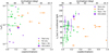 |
Fig. 6 Parameter space of the sample of debris disks. Here we show the HD 112810 debris disk (indicated with apurple star) compared to the sample of debris disks that have previously been imaged from the ground. Disks are color coded based on detection method: orange for polarized light only, purple for total intensity only, and green for detection in both polarized and total intensity. Left: fractional IR excess and on-sky inclination of disks; HD 112810 stands out as one of the least inclined disks imaged in total intensity. Right: modeled peak dust density (r0) and on-sky inclination of disks; in this case HD 112810 stands out as one of the largest disks to be imaged in scattered light, and is strikingly similar in geometry to HD131835, as well as the slightly larger disks surrounding HD141011 and 49 Ceti. Literature disk properties are from the ensemble of objects presented in Esposito et al. (2020) and from individual detections presented in Choquet et al. (2017); Bonnefoy et al. (2017, 2021); Sissa et al. (2018); Perrot et al. (2019, 2023); Hinkley et al. (2021); Lawson et al. (2021); Marshall et al. (2023). |
7.3 HD 112810 compared to the population of scattered light disks
In this section we consider how HD 112810 compares to the population of debris disks that have been detected in scattered light. Figure 6 shows the disk inclination, LIR/L⋆, and peak dust density of HD 112810 as compared to the sample of disks that have previously been observed from the ground in scattered light.
Even with an inclination of  , HD 112810 stands out as one of the least inclined disks to be detected in total intensity from the ground: only 49 Ceti (73 ± 3°), HD 117214
  and HD141011 (69.1 ± 0.9°) are less inclined (Choquet et al. 2017; Esposito et al. 2020; Bonnefoy et al. 2021, respectively). The disk has a similar inclination to the heavily studied HR 4796, as well as HD 129590. The bias of ADI-based disk detection towards very edge-on disks is well-known, so this is unsurprising, yet disks slightly further from edge-on are some of the most interesting for studying the disk SPF. For very edge-on disks, the grains with the smallest and largest scattering angles are obscured by the stellar PSF; further from the star, the front and back edges of the disk may be blended due to the stellar PSF. The geometry of moderate-inclination disks, meanwhile, is such that almost the entire range of scattering angles is accessible, with no parts of the disk obscured or blended. In the case of HD 112810, the SPF could be measured from ~15° to ~165°. Such moderate-inclination disks are therefore particularly useful for gaining insight into the grain physics within the disk, since a broader range of scattering angles are accessible, especially if the back edge of the disk is detected. Indeed, HR4796 has proved particularly intriguing for SPF studies (see e.g., Milli et al. 2017 for a detailed discussion). HD 112810 is sufficiently faint that such analysis is tricky with current data, but the disk is well-suited to SPF analysis with future facilities.
HD 112810 also stands out as one of the largest debris disks imaged in scattered light, with a radius of ~118 au. The disk radius and inclination are strikingly similar to that of the Sco-Cen object HD 131835, though that target has a much brighter fractional IR luminosity than HD 112810. As well as the polarimetric detection indicated in Fig. 6, HD 131835 was very recently detected in total intensity with SPHERE (Xie et al. 2022). Unlike HD 131835, HD 112810 has not yet been detected in polarized light. Note however that we have only presented total intensity images in this work; given the geometry and the low LIR/L⋆ of HD 112810, a polarized light detection would be challenging: the disk has a lower LIR/L⋆ than the majority of disks that have previously been detected in polarized light (Fig. 6), with only very edge-on disks being detected at fainter LIR/L⋆ values.
8 Conclusions
This paper has presented the first scattered light images of the HD 112810 debris disk, which we observed several times with VLT/SPHERE. Our key findings are as follows:
We detected the HD 112810 debris disk in scattered light, using H-band observations collected with the VLT/SPHERE/IRDIS high-contrast imaging platform. The signal is robust to our data processing approach, and is observed over several epochs of observations, but was not observed in the VLT/SPHERE/IFS observations in the YJ bands;
This disk is best fit with a single-belt debris disk, with a radius 118 ± 9 au and an inclination angle of
 . The detection is consistent with a single, narrow ring, but the signal-to-noise ratio of the disk is insufficient to adequately constrain the radial and vertical profile of the dust. This geometry is consistent with partially resolved ALMA images of the debris disk. The disk appears moderately forward scattering, with a Henyey-Greenstein forward scattering parameter 0.6 ± 0.1;
The disk lies towards the edge of the parameter space of disks that have been imaged in scattered light: it has a large radius, a moderate inclination, and a relatively low LIR/L⋆. This makes characterizing the disk challenging, but the disk geometry will allow for detailed study of the grain properties with future facilities;
No bound companions were detected in this system with direct imaging, astrometry or radial velocity. Smaller planets that remain undetectable (i.e., less than a few MJ, depending on orbital parameters and phase) could nonetheless be responsible for carving the observed debris disks structure.
HD 112810 adds to the growing inventory of scattered light disks, and extends the parameter space of the scattered light disk sample. The disk inclination of  could allow for the disk SPF to be measured between ~15°–165°. The debris disk is potentially amenable to imaging with the Hubble Space Telescope (HST), which would probe the faintest surface brightness material further from the star, and with future facilities such as the extremely large telescopes.
We searched the Gaia catalog out to a separation of 180″ (=24 000 au at the distance of HD112810). No sources with 5-parameter solutions have both parallax consistent with HD112810 to within 5σ, and proper motion consistent with HD112810 to within 5σ.
Updated values at https://www.pas.rochester.edu/~emamajek/EEM_dwarf_UBVIJHK_colors_Teff.txt
Acknowledgements
We thank the anonymous referee for the timely and thorough referee report, which improved the quality of this manuscript. Based on observations collected at the European Organisation for Astronomical Research in the Southern Hemisphere under ESO programme 0101.C-0016(A), with additional data from programmes 096.C-0713(C), 097.C-0949(A) and 097.C-0060(A), 098.C-0739(A) and 1101.C-0557(D). This work has made use of the SPHERE Data Centre, jointly operated by OSUG/IPAG (Grenoble), PYTHEAS/LAM/CESAM (Marseille), OCA/Lagrange (Nice), Observatoire de Paris/LESIA (Paris), and Observatoire de Lyon. We thank all the principal investigators and their collaborators who prepared and performed the observations with SPHERE. Without their efforts, we would not be able to build the master reference library to enable our RDI technique. This work has made use of data from the European Space Agency (ESA) mission Gaia (https://www.cosmos.esa.int/gaia), processed by the Gaia Data Processing and Analysis Consortium (DPAC, https://www.cosmos.esa.int/web/gaia/dpac/consortium). Funding for the DPAC has been provided by national institutions, in particular the institutions participating in the Gaia Multilateral Agreement. This research has made use of the SIMBAD database, operated at CDS, Strasbourg, France. This work has been carried out in part within the framework of the NCCR PlanetS supported by the Swiss National Science Foundation under grants 51NF40_182901 and 51NF40_205606. E.C.M. and W.C. acknowledge the financial support of the SNSF. C.D. acknowledges support from the European Research Council under the European Union’s Horizon 2020 research and innovation program under grant agreement No. 832428-Origins. This work has been supported by a grant from Labex OSUG (Investissements d’avenir – ANR10 LABX56). S.D. acknowledges support has been supported by the PRIN-INAF 2019 "Planetary systems at young ages (PLATEA)” and ASI-INAF agreement n.2018-16-HH.0. This work is supported by the French National Research Agency in the framework of the Investissements d'Avenir program (ANR-15-IDEX-02), through the funding of the “Origin of Life” project of the Univ. Grenoble-Alpes. B.B. acknowledges funding by the UK Science and Technology Facilities Council (STFC) grant no. ST/M001229/1. V.F.-G. acknowledges funding from the National Aeronautics and Space Administration through the Exoplanet Research Program under Grant No. 80NSSC21K0394 (PI: S. Ertel) This project is supported in part by the European Research Council (ERC) under the European Union’s Horizon 2020 research and innovation programme (COBREX; grant agreement no. 885593). F.Me. has received funding from the European Research Council (ERC) under the European Union’s Horizon Europe research and innovation program (grant agreement no. 101053020, project Dust2Planets). C.P. acknowledges funding from the Australian Research Council via FT170100040, DP180104235, and DP220103767. This research has made use of the NASA Exoplanet Archive, which is operated by the California Institute of Technology, under contract with the National Aeronautics and Space Administration under the Exoplanet Exploration Program. This work made use of Astropy (http://www.astropy.org): a community-developed core Python package and an ecosystem of tools and resources for astronomy (Astropy Collaboration 2013, 2018, 2022).
Appendix A Additional information for candidate companions
Five candidate companions were detected in Matthews et al. (2018) and re-detected in this work; these were assumed to be background objects in Matthews et al. (2018). We here confirm with common proper motion testing that these are indeed background objects. One new candidate companion is identified in this work towards the edge of the detector. This candidate is highly likely a background object, though additional data would be required to confirm this.
These candidates are all in the background-limited regime of the images, and a simple analysis of the IRDIS is sufficient to re-detect the companions and extract astrometry. We therefore derotated and co-added the cleaned image cubes from each epoch without applying PCA, and additionally co-added images from the two halves of the detector. We then determined the position of each candidate in each epoch by fitting the stellar PSF image to each companion, in a small box centered on the expected location of the candidate. The best-fitting position was converted into an on-sky astrometric acceleration, following the SPHERE User Manual6. We propagated uncertainties from the detector properties and from the stellar PSF fit to calculate astrometric errors. Astrometry for each candideate at each epoch is listed in Table A.1.
For the five companions detected in both 2016 and 2020, we compared the measured astrometry to predicted movement of a stationary background object between 2016-2020. We confirmed that all five sources are indeed background stars, as shown in Fig. A.1. Two of these five sources have since been detected in Gaia. One of these has a parallax confirming it as a background star while the other has a G-H2 color of ~1.3, implying a star mid-G spectral type – this is consistent with astrometric determination that this object is significantly more distant than HD 112810.
Astrometry for all candidate companions to HD 112810 identified in the VLT/SPHERE data.
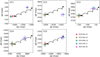 |
Fig. A.1 Companion astrometry overlaid on the background hypothesis for each of the candidate companions identified in 2016 data. In each case, colored points represent the measured position and 1σ uncertainty of the companion (also listed in Table A.1); the black trace indicates the long-term motion of an infinitely distant background companion, with black circles indicating positions at the observation epoch. All companions move broadly in the direction expected for a background object, though there is some scatter – implying a small proper motion of the background objects themselves. Considering the astrometry, as well as the wide separation (all >3.5″), all of these candidate companions are background objects. Companions CC2 and CC5 are also detected in the Gaia catalog, further confirming their identity as background objects. |
Appendix B Additional figures for the disk modeling
Here we include additional information for the disk modeling process, as described in Sect. 5. Specifically, Fig. B.1 shows the full corner plot for all the free parameters in the 5-parameter fit (Sect. 5.3, parameters are PA, itilt, r0, g, and ρ0). Corner plots are generated with corner.py (Foreman-Mackey 2016).
There is a clear correlation between the disk radius and the overall scaling of the disk: this is a natural result of the disk model setup (equation 1 above), where disk brightness falls with the square of distance from the star. To match the data, a larger disk needs a higher flux. These parameters are also correlated with the disk inclination, which is a natural result of the model disk geometry.
Figs. B.2 and B.3 show the full corner plot for the fits described in Sects. 5.4 and 5.5 respectively, overlaid on the 5-parameter fit. In each case we use dashed lines to indicate the values of fixed parameters in the 5-parameter fit. The ξ0 posterior follows the prior, while the αin and αout posteriors strongly favor very steep power laws, corresponding to a narrow disk. αin and αout are correlated with r0 and consequently also itilt, and the best fit values for these two parameters are ~ 1.5σ higher than for the 5-parameter fit.
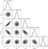 |
Fig. B.1 MCMC corner plot for the basic 5-parameter fit (Sect. 5.3), highlighting the key correlations present in the data. Note that we treat ρ0 as an arbitrary scaling factor. A clear correlation is observed between the disk inclination and characteristic radius, as is expected geometrically. The disk characteristic radius is also negatively correlated with the overall scaling factor ρ0, which is a natural consequence of the 1 /d2 scaling of scattered flux (see Equation 3). |
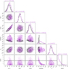 |
Fig. B.2 MCMC corner plot for the vertical structure fit (purple; Sect. 5.4) overlaid over the basic 5-parameter fit (black; Fig. B.1). The fixed value of ξ0 is indicated with a dashed black line. The ξ0 posterior follows the prior, and the parameter is strongly correlated with ρ0. All other parameters take similar values to the 5-parameter fit. We infer that the disk scale height ξ0 cannot be usefully inferred from the in-hand data. |
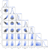 |
Fig. B.3 As Fig. B.2, but for the radial structure fit (blue; Sect. 5.5). The dashed black lines indicate the fixed values of αin and αout for the 5-parameter fit. The posterior for αout is moderatley constrained; for αin values ≲10 are strongly disfavored, but higher values follow the prior. We infer that the disk profile is steep, but the extent of the sharpness is hard to constrain. Notably, the r0 value is somewhat higher for this fit, as discussed in detail in Sect. 5.5. The disk inclination value is also higher in this case, following the clear correlation of r0 and itilt also highlighted in Fig. B.1. |
References
- Amara, A., & Quanz, S. P. 2012, MNRAS, 427, 948 [Google Scholar]
- Astropy Collaboration (Robitaille, T. P., et al.) 2013, A&A, 558, A33 [NASA ADS] [CrossRef] [EDP Sciences] [Google Scholar]
- Astropy Collaboration (Price-Whelan, A. M., et al.) 2018, AJ, 156, 123 [Google Scholar]
- Astropy Collaboration (Price-Whelan, A. M., et al.) 2022, ApJ, 935, 167 [NASA ADS] [CrossRef] [Google Scholar]
- Augereau, J. C., Lagrange, A. M., Mouillet, D., Papaloizou, J. C. B., & Grorod, P. A. 1999, A&A, 348, 557 [NASA ADS] [Google Scholar]
- Aumann, H. H. 1985, PASP, 97, 885 [Google Scholar]
- Barbato, D., Sozzetti, A., Desidera, S., et al. 2018, A&A, 615, A175 [NASA ADS] [CrossRef] [EDP Sciences] [Google Scholar]
- Beuzit, J. L., Vigan, A., Mouillet, D., et al. 2019, A&A, 631, A155 [NASA ADS] [CrossRef] [EDP Sciences] [Google Scholar]
- Boley, A. C., Payne, M. J., Corder, S., et al. 2012, ApJ, 750, L21 [NASA ADS] [CrossRef] [Google Scholar]
- Bonavita, M. 2020, Astrophysics Source Code Library [record ascl:2010.008] [Google Scholar]
- Bonnefoy, M., Milli, J., Ménard, F., et al. 2017, A&A, 597, A7 [NASA ADS] [CrossRef] [EDP Sciences] [Google Scholar]
- Bonnefoy, M., Milli, J., Menard, F., et al. 2021, A&A, 655, A62 [NASA ADS] [CrossRef] [EDP Sciences] [Google Scholar]
- Booth, M., Jordán, A., Casassus, S., et al. 2016, MNRAS, 460, L10 [NASA ADS] [CrossRef] [Google Scholar]
- Brandt, T. D. 2021, ApJS, 254, 42 [NASA ADS] [CrossRef] [Google Scholar]
- Bressan, A., Marigo, P., Girardi, L., et al. 2012, MNRAS, 427, 127 [NASA ADS] [CrossRef] [Google Scholar]
- Cantalloube, F., Mouillet, D., Mugnier, L. M., et al. 2015, A&A, 582, A89 [NASA ADS] [CrossRef] [EDP Sciences] [Google Scholar]
- Chen, C. H., Mamajek, E. E., Bitner, M. A., et al. 2011, ApJ, 738, 122 [NASA ADS] [CrossRef] [Google Scholar]
- Chen, C. H., Mittal, T., Kuchner, M., et al. 2014, ApJS, 211, 25 [Google Scholar]
- Choquet, É., Milli, J., Wahhaj, Z., et al. 2017, ApJ, 834, L12 [NASA ADS] [CrossRef] [Google Scholar]
- Claudi, R. U., Turatto, M., Gratton, R. G., et al. 2008, SPIE, 7014, 70143 [NASA ADS] [Google Scholar]
- Cotten, T. H., & Song, I. 2016, ApJS, 225, 15 [Google Scholar]
- Currie, T., Cloutier, R., Brittain, S., et al. 2015, ApJ, 814, L27 [Google Scholar]
- da Silva, L., Girardi, L., Pasquini, L., et al. 2006, A&A, 458, 609 [NASA ADS] [CrossRef] [EDP Sciences] [Google Scholar]
- Delorme, P., Meunier, N., Albert, D., et al. 2017, in SF2A-2017: Proceedings of the Annual meeting of the French Society of Astronomy and Astrophysics, eds. C. Reylé, P. Di Matteo, F. Herpin, et al. [Google Scholar]
- Desidera, S., Chauvin, G., Bonavita, M., et al. 2021, A&A, 651, A70 [EDP Sciences] [Google Scholar]
- de Zeeuw, P. T., Hoogerwerf, R., de Bruijne, J. H. J., Brown, A. G. A., & Blaauw, A. 1999, AJ, 117, 354 [Google Scholar]
- Dohlen, K., Langlois, M., Saisse, M., et al. 2008, SPIE, 7014, 70143 [NASA ADS] [Google Scholar]
- Engler, N., Lazzoni, C., Gratton, R., et al. 2020, A&A, 635, A19 [NASA ADS] [CrossRef] [EDP Sciences] [Google Scholar]
- Esposito, T. M., Kalas, P., Fitzgerald, M. P., et al. 2020, AJ, 160, 24 [Google Scholar]
- Feldt, M., Olofsson, J., Boccaletti, A., et al. 2017, A&A, 601, A7 [NASA ADS] [CrossRef] [EDP Sciences] [Google Scholar]
- Foreman-Mackey, D. 2016, J. Open Source Softw., 1, 24 [Google Scholar]
- Foreman-Mackey, D., Hogg, D. W., Lang, D., & Goodman, J. 2013, PASP, 125, 306 [Google Scholar]
- Gagné, J., Mamajek, E. E., Malo, L., et al. 2018, ApJ, 856, 23 [Google Scholar]
- Gaia Collaboration (Brown, A. G. A., et al.) 2021, A&A, 649, A1 [NASA ADS] [CrossRef] [EDP Sciences] [Google Scholar]
- Gaia Collaboration (Vallenari, A., et al.) 2023, A&A, 674, A1 [NASA ADS] [CrossRef] [EDP Sciences] [Google Scholar]
- Galicher, R., Boccaletti, A., Mesa, D., et al. 2018, A&A, 615, A92 [NASA ADS] [CrossRef] [EDP Sciences] [Google Scholar]
- Golimowski, D. A., Ardila, D. R., Krist, J. E., et al. 2006, AJ, 131, 3109 [NASA ADS] [CrossRef] [Google Scholar]
- Grandjean, A., Lagrange, A. M., Meunier, N., et al. 2023, A&A, 669, A12 [Google Scholar]
- Hagelberg, J., Ségransan, D., Udry, S., & Wildi, F. 2016, MNRAS, 455, 2178 [NASA ADS] [CrossRef] [Google Scholar]
- Hinkley, S., Matthews, E. C., Lefevre, C., et al. 2021, ApJ, 912, 115 [NASA ADS] [CrossRef] [Google Scholar]
- Hom, J., Patience, J., Esposito, T. M., et al. 2020, AJ, 159, 31 [NASA ADS] [CrossRef] [Google Scholar]
- Hughes, A. M., Duchêne, G., & Matthews, B. C. 2018, ARA&A, 56, 541 [Google Scholar]
- Hung, L.-W., Duchêne, G., Arriaga, P., et al. 2015, ApJ, 815, L14 [NASA ADS] [CrossRef] [Google Scholar]
- Jang-Condell, H., Chen, C. H., Mittal, T., et al. 2015, ApJ, 808, 167 [NASA ADS] [CrossRef] [Google Scholar]
- Janson, M., Brandt, T. D., Kuzuhara, M., et al. 2013, ApJ, 778, L4 [Google Scholar]
- Kalas, P. G., Rajan, A., Wang, J. J., et al. 2015, ApJ, 814, 32 [Google Scholar]
- Kasper, M., Apai, D., Wagner, K., & Robberto, M. 2015, ApJ, 812, L33 [NASA ADS] [CrossRef] [Google Scholar]
- Krivov, A. V. 2010, Res. Astron. Astrophys., 10, 383 [Google Scholar]
- Lafrenière, D., Doyon, R., Marois, C., et al. 2007, ApJ, 670, 1367 [Google Scholar]
- Lagrange, A.-M., Langlois, M., Gratton, R., et al. 2016, A&A, 586, A8 [NASA ADS] [CrossRef] [EDP Sciences] [Google Scholar]
- Lallement, R., Capitanio, L., Ruiz-Dern, L., et al. 2018, A&A, 616, A132 [NASA ADS] [CrossRef] [EDP Sciences] [Google Scholar]
- Lawson, K., Currie, T., Wisniewski, J. P., et al. 2021, AJ, 162, 293 [CrossRef] [Google Scholar]
- Lieman-Sifry, J., Hughes, A. M., Carpenter, J. M., et al. 2016, ApJ, 828, 25 [NASA ADS] [CrossRef] [Google Scholar]
- Lindegren, L., Hernández, J., Bombrun, A., et al. 2018, A&A, 616, A2 [NASA ADS] [CrossRef] [EDP Sciences] [Google Scholar]
- Lombart, M., Chauvin, G., Rojo, P., et al. 2020, A&A, 639, A54 [EDP Sciences] [Google Scholar]
- MacGregor, M. A., Wilner, D. J., Rosenfeld, K. A., et al. 2013, ApJ, 762, L21 [CrossRef] [Google Scholar]
- MacGregor, M. A., Weinberger, A. J., Nesvold, E. R., et al. 2019, ApJ, 877, L32 [NASA ADS] [CrossRef] [Google Scholar]
- Maire, A.-L., Langlois, M., Dohlen, K., et al. 2016, SPIE, 9908, 990834 [Google Scholar]
- Marino, S., Carpenter, J., Wyatt, M. C., et al. 2018, MNRAS, 479, 5423 [NASA ADS] [CrossRef] [Google Scholar]
- Marino, S., Yelverton, B., Booth, M., et al. 2019, MNRAS, 484, 1257 [NASA ADS] [CrossRef] [Google Scholar]
- Marino, S., Zurlo, A., Faramaz, V., et al. 2020, MNRAS, 498, 1319 [Google Scholar]
- Marois, C., Lafrenière, D., Doyon, R., Macintosh, B., & Nadeau, D. 2006, ApJ, 641, 556 [Google Scholar]
- Marshall, J. P., Milli, J., Choquet, E., et al. 2023, MNRAS, 521, 5940 [CrossRef] [Google Scholar]
- Matthews, B., Kennedy, G., Sibthorpe, B., et al. 2014, ApJ, 780, 97 [NASA ADS] [CrossRef] [Google Scholar]
- Matthews, E., Hinkley, S., Vigan, A., et al. 2017, ApJ, 843, L12 [NASA ADS] [CrossRef] [Google Scholar]
- Matthews, E., Hinkley, S., Vigan, A., et al. 2018, MNRAS, 480, 2757 [NASA ADS] [CrossRef] [Google Scholar]
- McDonald, I., Zijlstra, A. A., & Boyer, M. L. 2012, MNRAS, 427, 343 [Google Scholar]
- Mesa, D., Gratton, R., Zurlo, A., et al. 2015, A&A, 576, A121 [NASA ADS] [CrossRef] [EDP Sciences] [Google Scholar]
- Milli, J., Mouillet, D., Lagrange, A.-M., et al. 2012, A&A, 545, A111 [NASA ADS] [CrossRef] [EDP Sciences] [Google Scholar]
- Milli, J., Vigan, A., Mouillet, D., et al. 2017, A&A, 599, A108 [NASA ADS] [CrossRef] [EDP Sciences] [Google Scholar]
- Montalto, M., Piotto, G., Marrese, P. M., et al. 2021, A&A, 653, A98 [NASA ADS] [CrossRef] [EDP Sciences] [Google Scholar]
- Morrison, S., & Malhotra, R. 2015, ApJ, 799, 41 [NASA ADS] [CrossRef] [Google Scholar]
- Mouillet, D., Larwood, J. D., Papaloizou, J. C. B., & Lagrange, A. M. 1997, MNRAS, 292, 896 [Google Scholar]
- Mugnier, L. M., Cornia, A., Sauvage, J.-F., et al. 2009, J. Opt. Soc. Am. A, 26, 1326 [NASA ADS] [CrossRef] [Google Scholar]
- Pavlov, A., Möller-Nilsson, O., Feldt, M., et al. 2008, SPIE, 7019, 701939 [NASA ADS] [Google Scholar]
- Pawellek, N., & Krivov, A. V. 2015, MNRAS, 454, 3207 [Google Scholar]
- Pearce, T. D., Launhardt, R., Ostermann, R., et al. 2022, A&A, 659, A135 [NASA ADS] [CrossRef] [EDP Sciences] [Google Scholar]
- Pecaut, M. J., & Mamajek, E. E. 2013, ApJS, 208, 9 [Google Scholar]
- Pecaut, M. J., & Mamajek, E. E. 2016, MNRAS, 461, 794 [Google Scholar]
- Pecaut, M. J., Mamajek, E. E., & Bubar, E. J. 2012, ApJ, 746, 154 [Google Scholar]
- Perrot, C., Thebault, P., Lagrange, A.-M., et al. 2019, A&A, 626, A95 [NASA ADS] [CrossRef] [EDP Sciences] [Google Scholar]
- Perrot, C., Olofsson, J., Kral, Q., et al. 2023, A&A, 673, A39 [NASA ADS] [CrossRef] [EDP Sciences] [Google Scholar]
- Phillips, M. W., Tremblin, P., Baraffe, I., et al. 2020, A&A, 637, A38 [NASA ADS] [CrossRef] [EDP Sciences] [Google Scholar]
- Quillen, A. C. 2006, MNRAS, 372, L14 [NASA ADS] [CrossRef] [Google Scholar]
- Ratzenböck, S., Großschedl, J. E., Alves, J., et al. 2023, A&A, 678, A71 [NASA ADS] [CrossRef] [EDP Sciences] [Google Scholar]
- Ricci, L., Carpenter, J. M., Fu, B., et al. 2015, ApJ, 798, 124 [NASA ADS] [CrossRef] [Google Scholar]
- Rizzuto, A. C., Ireland, M. J., & Robertson, J. G. 2011, MNRAS, 416, 3108 [Google Scholar]
- Schneider, G., Smith, B. A., Becklin, E. E., et al. 1999, ApJ, 513, L127 [Google Scholar]
- Shannon, A., Bonsor, A., Kral, Q., & Matthews, E. 2016, MNRAS, 462, L116 [NASA ADS] [CrossRef] [Google Scholar]
- Sissa, E., Olofsson, J., Vigan, A., et al. 2018, A&A, 613, A6 [NASA ADS] [CrossRef] [EDP Sciences] [Google Scholar]
- Smith, B. A., & Terrile, R. J. 1984, Science, 226, 1421 [Google Scholar]
- Soummer, R., Pueyo, L., & Larkin, J. 2012, ApJ, 755, L28 [Google Scholar]
- Thébault, P. 2009, A&A, 505, 1269 [Google Scholar]
- Trifonov, T., Tal-Or, L., Zechmeister, M., et al. 2020, A&A, 636, A74 [NASA ADS] [CrossRef] [EDP Sciences] [Google Scholar]
- Vigan, A. 2020, Astrophysics Source Code Library [record ascl:2009.002] [Google Scholar]
- Vigan, A., Moutou, C., Langlois, M., et al. 2010, MNRAS, 407, 71 [Google Scholar]
- Vigan, A., Gry, C., Salter, G., et al. 2015, MNRAS, 454, 129 [NASA ADS] [CrossRef] [Google Scholar]
- Vigan, A., Bonnefoy, M., Ginski, C., et al. 2016, A&A, 587, A55 [NASA ADS] [CrossRef] [EDP Sciences] [Google Scholar]
- Wahhaj, Z., Liu, M. C., Biller, B. A., et al. 2014, A&A, 567, A34 [NASA ADS] [CrossRef] [EDP Sciences] [Google Scholar]
- Werner, M. W., Roellig, T. L., Low, F. J., et al. 2004, ApJS, 154, 1 [NASA ADS] [CrossRef] [Google Scholar]
- Wright, E. L., Eisenhardt, P. R. M., Mainzer, A. K., et al. 2010, AJ, 140, 1868 [Google Scholar]
- Wyatt, M. C. 2008, ARA&A, 46, 339 [Google Scholar]
- Wyatt, M. C., Dermott, S. F., Telesco, C. M., et al. 1999, ApJ, 527, 918 [Google Scholar]
- Xie, C., Choquet, E., Vigan, A., et al. 2022, A&A, 666, A32 [NASA ADS] [CrossRef] [EDP Sciences] [Google Scholar]
- Yelverton, B., & Kennedy, G. M. 2018, MNRAS, 479, 2673 [NASA ADS] [CrossRef] [Google Scholar]
- Zurlo, A., Vigan, A., Mesa, D., et al. 2014, A&A, 572, A85 [NASA ADS] [CrossRef] [EDP Sciences] [Google Scholar]
All Tables
Astrometry for all candidate companions to HD 112810 identified in the VLT/SPHERE data.
All Figures
|
Fig. 1 SPHERE/IRDIS images of the HD 112810 debris disk. Each column indicates data processed via a different method: GRAPHIC/PCA (Sect. 4.1; Hagelberg et al. 2016), TLOCI as provided by the SPHERE data center (Sect. 4.2; Delorme et al. 2017) or RDI (Sect. 4.3; Xie et al. 2022); rows indicate each observation epoch. In each case, the two SPHERE/IRDIS channels are co-added. There are no RDI reductions for the BB_H data, since there is far more data collected with the DB_H23 filter in the archive, and the reference library we considered does not collate BB_H data (Xie et al. 2022). The “normalized signal” is calculated relative to the background noise in the wide-field; we note that this is not a true S/N at very small separations, where the noise is higher than the background limit. |
| In the text | |
|
Fig. 2 SPHERE/IFS reduced data for HD 112810. Here, we show an image with all data epochs and all wavelengths co-added, with the GRAPHIC/PCA (left) and ANDROMEDA (right) algorithms applied to remove stellar speckles. In both cases, these are S/N maps; for GRAPHIC/PCA each annulus is scaled by the variance in that annulus, causing sharp transitions between concentric annuli. We tried several data reduction approaches and varied the values of tuned parameters. While a few bright spots are seen very close to the inner working angle, these are detected at low significance and are not at consistent locations between epochs – indicating that these are residual stellar speckles. The disk signal is not visible in any IFS data, either in the individual or in the co-added epochs. |
| In the text | |
|
Fig. 3 Best fitting models to the data, alongside the raw data and the residual image with the disk subtracted. 3- and 5-σ contours (relative to the background noise) are shown in pink and purple respectively. The three rows show the best fitting models for (a) the 5-parameter fit (b) the vertical structure fit, and (c) the radial structure fit (see Sects. 5.3–5.5). Best-fit parameters are given in Table 2. Residual images are generated by subtracting model disks from the raw data, and then repeating the PCA reduction. The debris disk is well-subtracted in all cases. |
| In the text | |
|
Fig. 4 Contrast (left) and mass sensitivities (right) of each epoch of observations. The legend applies to both figures; cool colors indicate the narrowband DB_H23 observations and warm colors indicate the broadband BB_H observations. Companion magnitude limits were converted to mass limits using the ATMO models from Phillips et al. (2020). |
| In the text | |
|
Fig. 5 Detection completeness for HD 112810. Shaded rows show completeness for radial velocity observations (blue), HIPPARCOS-Gaia proper motion analysis (pink), and high-contrast imaging observations (green) along with the debris belt positions (gray). Shaded regions indicate the mass vs separation contours at which 10%, 50%, 90% and 99% of companions would be detectable with in-hand data, as described in Sects. 6.3, 6.4 and 6.1 respectively. The inner and outer belt positions are derived from the SED fit and SPHERE modeling respectively. Planetary mass companions and small brown dwarfs at intermediate and wide separations are largely ruled out from the proper motion and imaging constraints. The radial velocity constraints are weaker, ruling out only massive stellar companions at short periods. |
| In the text | |
|
Fig. 6 Parameter space of the sample of debris disks. Here we show the HD 112810 debris disk (indicated with apurple star) compared to the sample of debris disks that have previously been imaged from the ground. Disks are color coded based on detection method: orange for polarized light only, purple for total intensity only, and green for detection in both polarized and total intensity. Left: fractional IR excess and on-sky inclination of disks; HD 112810 stands out as one of the least inclined disks imaged in total intensity. Right: modeled peak dust density (r0) and on-sky inclination of disks; in this case HD 112810 stands out as one of the largest disks to be imaged in scattered light, and is strikingly similar in geometry to HD131835, as well as the slightly larger disks surrounding HD141011 and 49 Ceti. Literature disk properties are from the ensemble of objects presented in Esposito et al. (2020) and from individual detections presented in Choquet et al. (2017); Bonnefoy et al. (2017, 2021); Sissa et al. (2018); Perrot et al. (2019, 2023); Hinkley et al. (2021); Lawson et al. (2021); Marshall et al. (2023). |
| In the text | |
|
Fig. A.1 Companion astrometry overlaid on the background hypothesis for each of the candidate companions identified in 2016 data. In each case, colored points represent the measured position and 1σ uncertainty of the companion (also listed in Table A.1); the black trace indicates the long-term motion of an infinitely distant background companion, with black circles indicating positions at the observation epoch. All companions move broadly in the direction expected for a background object, though there is some scatter – implying a small proper motion of the background objects themselves. Considering the astrometry, as well as the wide separation (all >3.5″), all of these candidate companions are background objects. Companions CC2 and CC5 are also detected in the Gaia catalog, further confirming their identity as background objects. |
| In the text | |
|
Fig. B.1 MCMC corner plot for the basic 5-parameter fit (Sect. 5.3), highlighting the key correlations present in the data. Note that we treat ρ0 as an arbitrary scaling factor. A clear correlation is observed between the disk inclination and characteristic radius, as is expected geometrically. The disk characteristic radius is also negatively correlated with the overall scaling factor ρ0, which is a natural consequence of the 1 /d2 scaling of scattered flux (see Equation 3). |
| In the text | |
|
Fig. B.2 MCMC corner plot for the vertical structure fit (purple; Sect. 5.4) overlaid over the basic 5-parameter fit (black; Fig. B.1). The fixed value of ξ0 is indicated with a dashed black line. The ξ0 posterior follows the prior, and the parameter is strongly correlated with ρ0. All other parameters take similar values to the 5-parameter fit. We infer that the disk scale height ξ0 cannot be usefully inferred from the in-hand data. |
| In the text | |
|
Fig. B.3 As Fig. B.2, but for the radial structure fit (blue; Sect. 5.5). The dashed black lines indicate the fixed values of αin and αout for the 5-parameter fit. The posterior for αout is moderatley constrained; for αin values ≲10 are strongly disfavored, but higher values follow the prior. We infer that the disk profile is steep, but the extent of the sharpness is hard to constrain. Notably, the r0 value is somewhat higher for this fit, as discussed in detail in Sect. 5.5. The disk inclination value is also higher in this case, following the clear correlation of r0 and itilt also highlighted in Fig. B.1. |
| In the text | |
Current usage metrics show cumulative count of Article Views (full-text article views including HTML views, PDF and ePub downloads, according to the available data) and Abstracts Views on Vision4Press platform.
Data correspond to usage on the plateform after 2015. The current usage metrics is available 48-96 hours after online publication and is updated daily on week days.
Initial download of the metrics may take a while.