| Issue |
A&A
Volume 679, November 2023
|
|
|---|---|---|
| Article Number | A53 | |
| Number of page(s) | 13 | |
| Section | Catalogs and data | |
| DOI | https://doi.org/10.1051/0004-6361/202245434 | |
| Published online | 03 November 2023 | |
VLBI celestial and terrestrial reference frames VIE2022b
1
Technische Universität Wien (TU Wien), Department of Geodesy and Geoinformation,
Wiedner Hauptstraße 8–10,
1040
Vienna, Austria
e-mail: This email address is being protected from spambots. You need JavaScript enabled to view it.
2
Federal Office of Metrology and Surveying (BEV),
Schiffamtsgasse 1–3,
1020
Vienna, Austria
Received:
11
November
2022
Accepted:
12
August
2023
Abstract
Context. We present the computation of global reference frames from very long baseline interferometry (VLBI) observations at the Vienna International VLBI Service for Geodesy and Astrometry (IVS) Analysis Center (VIE) in detail. We focus on the celestial and terrestrial frames from our two latest solutions VIE2020 and VIE2022b.
Aims. The current international celestial and terrestrial reference frames, ICRF3 and ITRF2020, include VLBI observations until March 2018 (at the standard geodetic and astrometric radio frequencies 2.3 and 8.4 GHz) and December 2020, respectively. We provide terrestrial and celestial reference frames including VLBI sessions until June 2022 organized by the IVS.
Methods. Vienna terrestrial and celestial reference frames are computed in a common least squares adjustment of geodetic and astro-metric VLBI observations with the Vienna VLBI and Satellite Software (VieVS).
Results. We provide high-precision celestial and terrestrial reference frames computed from 24 h IVS observing sessions. Our latest celestial reference frame solution VIE2022b-sx provides positions of 5407 radio sources at the frequency of 8.4 GHz. In particular, the positions of sources with few observations at the time of the ICRF3 calculation are improved. The frame also includes positions of 870 radio sources not included in ICRF3. The additional observations beyond the data used for ITRF2020 provide a more reliable estimation of positions and linear velocities of newly established VLBI Global Observing System (VGOS) telescopes.
Key words: methods: data analysis / techniques: interferometric / catalogs / astrometry / reference systems
© The Authors 2023
 Open Access article, published by EDP Sciences, under the terms of the Creative Commons Attribution License (https://creativecommons.org/licenses/by/4.0), which permits unrestricted use, distribution, and reproduction in any medium, provided the original work is properly cited.
This article is published in open access under the Subscribe to Open model. This email address is being protected from spambots. You need JavaScript enabled to view it. to support open access publication.
1 Introduction
Geodetic and astrometric very long baseline interferometry (VLBI) observations have been carried out since 1979. Since 1999, the VLBI sessions – from scheduling to analysis – have been organized by the International VLBI Service for Geodesy and Astrometry (IVS; Nothnagel et al. 2017). The Vienna IVS Analysis Center (VIE), jointly operated by TU Wien and the Federal Office of Metrology and Surveying (BEV) in Austria, is one of the eight institutions worldwide that actively contributed to studies needed for the latest update of the international celestial reference frame (ICRF), generating one of the prototype realizations of the current ICRF3 (Charlot et al. 2020), which was adopted by the International Astronomical Union in August 2018.
Furthermore, VIE, as one of the IVS analysis centers, participated in recent international efforts to calculate an updated realization of the international terrestrial reference system (ITRS). VIE analyzed a complete set of individual VLBI observing sessions and provided pre-reduced normal equation systems (NEQs) for combination with results of other IVS analysis centers at the IVS Combination Center (Hellmers et al. 2022). The final international terrestrial reference frame (ITRF) originates from the combination of reprocessed solutions from four space geodetic techniques (Doppler orbitography by radiopositioning integrated on satellite, global navigation satellite systems, satellite laser ranging (SLR), and VLBI). This final combination allows to overcome the weaknesses of individual techniques taking advantage of the strength of a combined solution. The current version of the ITRF, the ITRF2020 (Altamimi et al. 2022), was published in April 2022.
Besides our support of the international efforts toward conventional reference frame realizations, we generate our own global VLBI reference frames. The celestial and terrestrial reference frames, together with the connecting Earth orientation parameters (EOPs), are created in a common least squares adjustment of VLBI observations using the Vienna VLBI and Satellite Software version 3.3 (VieVS; Böhm et al. 2018). In this paper, we introduce our global reference frame solution VIE2020 generated with VLBI observing sessions as provided for the ITRF2020 computations. Furthermore, we also focus on our recent global solution VIE2022b, which involves VLBI sessions released after the ITRF2020 cutoff date. In total, this solution includes VLBI data from an additional 18 months compared to ITRF2020. In Sect. 2, we describe the VLBI data in detail and give information about the a priori models and parametrization of the solutions. Extensive descriptions of the estimated terrestrial and celestial reference frames, including comparisons to the most recent international reference frames, are given in Sects. 3 and 4, respectively. A brief summary of content of this paper is provided in Sect. 5.
2 Data and analysis settings
We analyze VLBI group delays, which are fundamental observables of geodetic and global astrometric VLBI. In the IVS operation scheme (Nothnagel et al. 2017), after correlation, fringe fitting, and pre-processing, the group delays are provided in databases in the IVS vgosDB format (Gipson & IVS Working Group IV on Data Structures 2021) via IVS data centers. In VieVS, we start with databases which include group delays at X-band (8.4 GHz) with ambiguities resolved and the ionospheric delays calibrated with a linear combination with simultaneous S -band (2.3 GHz) measurements.
The basis of our data analysis consists of VLBI sessions observed at S/X frequencies, which were analyzed for the ITRF2020 contribution by the IVS. In addition, we include 467 S/X weak-network sessions (with two or three stations only), which were scheduled mainly for astrometric purposes to strengthen the ICRF in the Southern Hemisphere (see special handling of EOPs at end of section). They were also part of the ICRF3 solution. Furthermore and most importantly, for this publication the dataset has been extended to include observation sessions arriving after the ITRF2020 cutoff date, that is, from January 2021 until June 2022.
It should also be noted that in recent years, the geodetic VLBI technique has been undergoing a transition phase from a legacy S/X era to a novel VLBI Global Observing System (VGOS; Petrachenko et al. 2009). The VGOS system allows broadband observations, which may employ four frequency bands covering the range from 2 GHz to 14 GHz. Up to now, the four bands are located in the ranges of 3–3.5, 5.3–5.8, 6.4–6.9, and 10.2–10.7 GHz. The ITRF2020 solution includes VGOS sessions1 together with S/X sessions2. This enables consistent estimation of the coordinates for newly built VGOS telescopes within the ITRF. On the other hand, if a global solution is computed with a primary focus on the celestial reference frame, the mixture of observations at different frequencies is not desirable.
For this reason, we constructed two solutions with the input to ITRF2020 including the 467 S/X weak-network sessions, one with and one without VGOS sessions, denoted hereafter as VIE2020 and VIE2020-sx, respectively. With the augmentation by the January 2021 to June 2022 data, we then set up two additional solutions, again one with and one without VGOS sessions denoted as VIE2022b and VIE2022b-sx, respectively (see Table 1). There are 7148 VLBI sessions in the VIE2022b solution, providing 22.4 million observations in total. The solution VIE2022b-sx is built with 21.6 million observations, which makes a difference of 0.8 million observations in 90 VGOS sessions, each of 24 h.
In Table 2, we provide an overview of the a priori models used for the calculation of the VLBI theoretical delays in the VIE2020 and VIE2022b solutions. The only difference is the choice of the a priori terrestrial reference frame (TRF): VIE2020 is based on ITRF2014 with no-net-rotation (NNR) and no-nettranslation (NNT) conditions, whereas VIE2022b is based on ITRF2020.
As a side note, we want to emphasize the importance of the consistent use of tropospheric mapping functions for the hydrostatic and wet parts of the tropospheric delays. More specifically, we carried out an analysis of our submission to the ITRF2020 with the aim being to investigate the reason for the mean scale difference of 0.2 ppb between our solution (VIE) and ITRF2014 compared to a range from 0.3 to 0.5 ppb for the other IVS Analysis Centers (compare Fig. 12 by Hellmers et al. 2022). We find that applying VMF3 (Landskron & Böhm 2018) to model the hydrostatic part of the tropospheric delays and VMF1 (Böhm et al. 2006) to model the wet part causes the estimated baseline lengths between two telescopes to be 2 mm shorter on average compared to using VMF1 or VMF3 for both constituents consistently. The subsequent comparison of two global solutions reveals that the difference in baseline length causes an offset in the scale of the estimated global TRFs of about 0.3 ppb. In-depth analyses are ongoing.
The weighting of the data applied in our ITRF2020 submission follows the standard approach in VLBI analysis known as global weighting. The standard deviation of each observation derived from the fringe fitting process is inflated by a constant value to avoid the formal errors of the observations being unrealistically small. In our ITRF2020 submission, we add a value of 17 ps in a root sum square sense to the noise of each observation. In the VIE2020 and VIE2022b solution, we introduce elevation-dependent noise instead of a global constant value. The standard deviation of each observation σobs is obtained from Eq. (1) (Gipson et al. 2008):
 (1)
(1)
where σ0 consists of a measurement noise σm plus an ionospheric delay formal error  . The elevationdependent noise terms for stations i and j, σi and σj, are computed with a constant xi, j = 6 ps for each station divided by the sine of the associated elevation angle ε. Hence, observations at lower average elevations obtain a lower weight in the least squares adjustment. The noise coefficient of 6 ps is a value recommended by Gipson et al. (2008), which provided the greatest reduction of the baseline length scatter for the continuous two-week VLBI campaign CONT053.
Operational data processing with VieVS consists of two steps providing a first solution and a main solution. In the first solution, a pre-analysis of the VLBI sessions with a basic parametrization is carried out to check for possible problematic behavior of the data. In the majority of cases, this can be solved with an individual single session parametrization; for example, the definition of clock breaks, exclusion of cable calibration signals at stations, removal of large outliers, and removal of measurements at individual antennas or baselines, if unavoidable. This configuration, with even more possible options for each VLBI session, is stored in the VieVS-internal OPT-flles4, which we provide to the public.
As a next step, the parametrization of the main solution is configured (see Table 3). In the software package VieVS, the parametrization of the time-variable unknowns is realized with piece-wise linear offsets (PWLOs) with certain time intervals and relative constraints between the offsets. The single session least-squares adjustment, is also important for identifying baseline-dependent clock offsets (BCOs; Krásná et al. 2021) in the network. The baselines with an estimated clock offset larger than three times its formal error are listed in the OPT-files for estimation in the final solution.
Next, session-wise NEQs are prepared for the final global adjustment. After the reduction, these NEQs only contain parameters that are constant over several VLBI sessions, and will be estimated globally. The parameters that are time-dependent and do not benefit from long time series of observations are squeezed out from the NEQs. In our solutions, we estimate session-wise (baseline-dependent) clock parameters, zenith wet delays, tropospheric gradients in the north and east directions at individual stations, and the coordinates of telescopes that observed only occasionally within our dataset. The Earth rotation parameters (ERPs; i.e., polar motion and UT1-UTC) are estimated session-wise for networks with more than three telescopes. For the small networks of three stations or single baselines, all five Earth orientation parameters are fixed to a priori International Earth Rotation and Reference Systems Service (IERS) Bulletin A values issued by the IERS Rapid Service/Prediction Center at the U.S. Naval Observatory (USNO).
The adjustment of the set of sessions is applied to a normal equation system, which results from stacking the individual NEQs according to the theorem of stacking pre-reduced normal equation systems by Helmert (see, e.g., Brockmann 1997). The set of global parameters determined by the common inversion of the stacked NEQs then only contains coordinates and velocities of telescopes, amplitudes of annual and semi-annual displacements in the station height of selected stations, and positions of radio sources.
Overview of solutions described in this publication.
A priori models used in the VIE2020 and VIE2022b solutions.
3 Vienna terrestrial reference frame
Producing a new global TRF requires detailed information about the underlying dataset and in particular about the observation time of telescopes taking part in the observation schedules. A traditional TRF catalog consists of station coordinates at a given epoch and the linear velocities of the stations. The determination of the velocity requires a sufficiently long observation time period with the telescope in order to enable the estimation of the linear movement predominantly caused by plate tectonics.
For this reason, we set a lower limit of 15 VLBI sessions including the station and a minimum time span of 5 yr between the first and last observations. For telescopes not fulfilling these conditions, the coordinates are determined as the average of the position time series estimated from the individual sessions. Exceptions to this rule are telescopes at common sites with other VLBI telescopes, where the velocities are constrained to be identical with respect to the same a priori velocities. The definition of interval breaks because of discontinuous station movements (mainly by Earthquakes or by service work changing the reference position of the telescope) is taken from the a priori catalog, that is, ITRF20145 and ITRF20206 for VIE2020 and VIE2022b solutions, respectively. The modeling of the nonlinear motion caused by post-seismic deformation is based on the logarithmic and exponential functions given in the a priori ITRF catalogs. Table 4 summarizes the pairs (or groups) of telescopes tied together in solution VIE2022b.
To align the solutions to the a priori frame, NNT/NNR conditions are applied to the coordinates and velocities of a set of 21 stable telescopes with a long observation history: ALGOPARK, BR-VLBA, FD-VLBA, FORTLEZA, HARTRAO, HN-VLBA, HOBART26, KASHIMA, KOKEE, KP-VLBA, LA-VLBA, MATERA, NL-VLBA, NOTO, NYALES20, ONSALA60, OV-VLBA, SC-VLBA, SVETLOE, WESTFORD, WETTZELL. The reference epoch is set to January 1, 2015, for both frames, VIE2020 and VIE2022b, for consistency with the reference epoch of ITRF2020. Figure 1 shows the activity of telescopes observing in more than 50 sessions in VIE2022b as a function of time. The red crosses indicate the breaks in position or velocity taken from ITRF2020.
In addition, we estimated the seasonal displacement in the height component at annual and semi-annual periods Pi (P1 = 365.25 days, P2 = 182.63 days) at selected stations. The station height displacement ∆h = ∆h1 + ∆h2 is parametrized in a form of sine and cosine amplitudes (Asi, Aci):
 (2)
(2)
where the reference epoch mjd0 is set to January 1, 2015, and mjd is the modified Julian date of the session. The amplitude Ai and phase ϕi of the seasonal wave are obtained with the basic mathematical relation as:
 (3)
(3)
We estimate these parameters at 74 antennas, which took part in at least 50 sessions, and where the measurements cover the changing seasons. Thus, we do not estimate the seasonal displacement for EFLSBERG, OHIGGINS, PARKES, SYOWA, and YLOW7296 because their participation in VLBI sessions is rather episodic (cf. Fig. 1). The estimation of the amplitude for a semi-annual signal is relevant especially for telescopes in the subtropical zones, where the sum of the annual and semiannual signal best fits the changes in the telescope height over a year. The estimated annual and semi-annual signals for all 74 telescopes are plotted in Fig. 2 as arrows representing the amplitude (length) and the time of the maximum height displacement (phase, north = Jan. 1). In Table 5, we highlight the estimates of the seasonal (annual and semi-annual) signal at the newly established VGOS antennas and complete the information with the legacy telescopes at the common sites. The accuracy of the estimated signal depends on the number and distribution of the sessions allowing the correct tracing of the height change over the year. For example, in Europe, the maximum reading of the annual signal in height occurs in the summer months of July and August, which means that the crust moves up. At observatories in Onsala or Wettzell, there is an agreement between the seasonal height changes estimated at all telescopes with a positive maximum of 4–6 mm occurring in July. This can be explained by the minimal water content in the ground and the lack of snow load, as we applied neither the seasonal signal provided for ITRF2014 or ITRF2020 nor any hydrology loading modeling in the data analysis. These results agree with former findings published for example by Tesmer et al. (2009) or Krásná et al. (2015).
On the other hand, there are differences of several millimeters in the amplitudes of the seasonal signals between telescopes at some common sites, such as GGAO12M and GGAO7108, NYALES13S and NYALES20, or RAEGYEB and YEBES40M. In our solution, we do not apply any constraints on the seasonal signal at the telescopes close to each other. There can be several reasons for the overestimation of the amplitudes of the seasonal signal at the stations. In the case of GGAO7108 and YEBES40M, we assume that the reason is connected to the noisy height time series of the telescopes, especially after the year 2003 at GGAO71087, and prior to the year 2017 at YEBES40M8. In a footnote, we provide links to the position time series provided by the ITRF2020 team, which show approximately the same pattern as our time series. In the case of NYALES13S, which started to participate in the IVS sessions in February 2020, there is a gap in observations of four months from July to November 2020 causing an inhomogeneous distribution of the observations over time. For comparison, Table 5 includes the amplitude and phase for annual and semi-annual signals in height computed from the sine and cosine amplitudes as they are provided with ITRF20209. ITRF2020 contains identical signals at all telescopes at the sites listed in Table 5. The only exception is telescope NYALE13S, where the amplitude of the seasonal signal is set to zero in the ITRF2020 and should be treated carefully in analyses.
In addition to the seasonal signal in station height at VGOS antennas in VJE2O22b and ITRF2020 in Table 5, the height differences at epoch 2015.0 and the differences in height velocity computed as VIE2022b minus ITRF2020 are listed in Table 6 (second and third columns). The respective formal errors m∆h and m∆ḣ of the differences are computed by propagating the uncertainties from both catalogs. In columns four to seven, we show the formal errors of the height components separately for VIE2022b, ITRF2020, and in brackets for VIE2020. In the last column, we present the number of sessions included in ITRF2020 for telescopes that started their observations after November 2017 (cf. Fig. 1) as obtained from the published ITRF2020 station time series at the ITRF website10. The height difference at these new stations is mainly the consequence of having more data available in VIE2022b (cf. with number of sessions in Table 5). To show the positive impact of the new sessions observed after December 2020 on the formal errors of the estimated height directly, we include the formal errors of VIE2022b and VIE2020 in Table 6. Their comparison shows a lower height error in VJE2O22b for all concerned stations. (The positions of telescopes RAEGSMAR and MACG012M were estimated session-wise in the VIE2020 solution due to the low number of available sessions). These TRF formal errors from the VJE solutions are a rough output of the VLBI data analysis. They are not scaled, nor is there a noise floor added to them. Apart from the newest telescopes, there is a height difference at epoch 2015.0 of several centimeters between VIE2022b and ITRF2020 at two legacy telescopes, GGAO7108 and HRAS_O85, which stopped their observations in 2007 and 1990, respectively. We assume that the reason is the noisy position time series of these two telescopes, which may hamper the extrapolation of the height difference. In the case of GGAO7108, the noise in the height time series is reflected in the large formal errors of the height component in both solutions, that is VJE2O22b (10.6 mm) and ITRF2020 (28.7 mm). In the case of HRAS_O85, the formal error of the height position component in VJE2O22b is 17.1 mm, while in ITRF2020 it is 3.3 mm. Contamination of the HRAS_O85 position time series with a spurious signal was already reported and studied by several authors, for example by Iz & Chen (1999). Due to this anomalous behavior and noise in the position time series of HRAS_O85, we do not apply velocity ties to the FD-VLBA telescope even though the distance between the telescope positions is 0.30 km. The estimation of the velocity at HRAS_O85 without ties to FD-VLBA explains the large formal error in VJE2O22b (0.62 mm/yr) for the height velocity component of HRAS_O85. This error, estimated from the VLBI data collected in the 1980s, propagates through the extrapolation of the position to the epoch 2015.0.
At most telescopes, the estimated heights are larger in VJE2O22b than in ITRF2020. In particular, this is true for all differences exceeding their formal error and telescopes observing in the final years. At ISHIOKA, the height difference at epoch 2015.0 is −6.4 ± 1.7 mm but the difference in height velocity is 1.6 ± 0.4 mm yr−1 between VJE2O22b and ITRF2020. We assume that the reason is the active tectonics in the Ishioka area. To illustrate the effect of larger heights in VIE2022b, we show the session-wise scale factor of the VIE2022b parametrization with respect to ITRF2020 in Fig. 3. After 2014, there is a trend in the smoothed line that reflects the increasing scale difference between the TRF estimated from VLBI observations only and the ITRF. The ITRF2020 relies in its scale definition on two space geodetic techniques, namely VLBI and SLR. The scale of the ITRF2020 long-term frame was determined using internal constraints in such a way that there is zero difference between the scale and scale rate of ITRF2020 and the scale and scale rate averages of VLBI selected sessions up to 2013.75 (see ITRF2020 webpage11). A VLBI working group under the lead of the IVS Analysis Coordinator has been established to investigate this phenomenon.
Table 7 summarizes the 14 transformation parameters (three translation parameters (Tx, Ty, Tz), three rotation parameters (Rx, Ry, Rz), and one scale factor, each with its time derivative) at epoch 2015.0 from ITRF2020 to VIE2020 (top lines), and from ITRF2020 to VIE2022b (bottom lines). The parameters are computed from stations with mean coordinate errors mxyz (Eq. (4)) of lower than 10 mm in VIE2020 and VIE2022b, respectively:
 (4)
(4)
where  ,
,  , and
, and  are the formal errors of the coordinates. The maximum translation of −3.4 ± 1.7 mm occurs in the y-direction between VIE2020 and ITRF2020 but it is still within a factor of three of its formal error. The remaining translation parameters are negligible. All rotations are close to or below their formal errors and the maximum value of 60.5 ± 69.2 µas appears in the x-direction between VIE2020 and ITRF2020. The scale factors from the Vienna VLBI TRFs VIE2020 and VIE2022b show differences of 0.56 ± 0.26 ppb and 0.59 ± 0.11 ppb with respect to ITRF2020, respectively.
Parametrization of the VIE2020 and VIE2022b solutions.
VLBI telescopes in VIE2022b at common sites where velocity ties are applied.
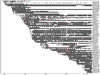 |
Fig. 1 Antenna participation in VLBI sessions in solution VIE2022b. Red crosses depict the placement of position breaks. Only antennas included in more than 50 sessions are plotted. |
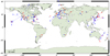 |
Fig. 2 Annual (blue) and semi-annual (red) height signal in VIE2022b. The amplitude is depicted by the arrow length. The phase of the maximum displacement is represented by the orientation of the arrow. If the arrow points toward north, the maximum appears in January and continues clockwise thereafter. The maximum of the semi-annual signal is depicted in the first half year. |
Seasonal signal in station height of new VGOS antennas and legacy antennas at common sites.
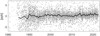 |
Fig. 3 Session-wise scale factor computed with VIE2022b parametrization with respect to ITRF2020. The black line represents the smoothed scale factor obtained by local regression using a span of 5% of the total number of data points. |
Transformation parameters at epoch 2015.0 between TRFs.
4 Vienna celestial reference frame
Celestial reference frames (CRFs) are estimated in common global solutions together with the TRFs. We focus on the CRF, including the most recent geodetic and astrometric VLBI sessions until June 2022 observed at S/X frequencies. The catalog VIE2022b-sx consists of 5407 radio sources. All sources present in the underlying data are kept in the analysis and their positions are estimated as global parameters. This means that we neither remove gravitational lenses from the solution, as was done in ICRF3, nor estimate sources with nonlinear motions as session-wise parameters (“special handling” sources in ICRF2, Fey et al. 2015). We use ICRF3 as the a priori frame and model the Galactic acceleration correction with the adopted ICRF3 value of AG = 5.8 µas yr−1 for the amplitude of the Solar System barycenter acceleration vector in the direction of the Galactic center (right ascension αGC = 266.4°, declination δGC = −28.94°) for the epoch 2015.0.
The alignment of the new CRF to the a priori one is accomplished via defining sources. In ICRF3, a new set of defining sources was selected (independent of ICRF2 defining sources) based on several criteria, one of them being a uniform distribution on the sky. Because of the generally sparser distribution of the observed radio sources in the far south, sources with lower position stability or a low number of observations had to be included in the set of defining sources. We divide the 303 ICRF3 defining sources into three groups so that we include every third source from the ICRF3 defining source list sorted in ascending order according to their right ascension. We then compute three global solutions, which we align to ICRF3 with unweighted NNR constraints (Jacobs et al. 2010) applied to coordinates of the 101 ICRF3 defining sources included in the three independent lists. Figure 4 shows the differences in estimated source coordinates α* and δ with respect to a solution where all 303 ICRF3 defining sources are in the NNR condition. We use the designation α* for right ascension scaled by declination of the source, that is, α* = α · cos δ. Each color (red, green, and blue) represents one of the global solutions aligned with the subgroup of 101 ICRF3 defining sources. A systematic difference in the estimated coordinates when excluding 202 radio sources from the NNR condition is evident with the peak of the differences at around 20 µas for both coordinates. In particular, we identify two radio sources with a difference in the estimated coordinates above 1 mas when dropped from the NNR condition (0700-465, ∆α* = 3.9 mas, ∆δ = 3.5 mas; 0809-493, ∆α* = 4.2 mas, ∆δ = 1.7 mas). Therefore, we do not use them to align our Vienna CRFs (black dots in Fig. 4 for VIE2022b-sx) to ICRF3. The source 0700-465 has 45 observations in ICRF3 with the first one in September 1990 and 80 observations in VIE2022b-sx. The source 0809-493 was observed in June 1990 for the first time and has 22 observations in ICRF3 and 30 in VIE2022b-sx.
We depict the number of new observations for ICRF3 defining sources in Fig. 5 and nondefining sources in Fig. 6 after the ICRF3 cutoff (March 27, 2018) until June 23, 2022. The majority of new observations for the deep south sources (δ < −45°) come from three dedicated programs: astrometric IVS Celestial Reference Frame Deep South sessions (IVS-CRDS; de Witt et al. 2019; Weston et al. 2023), sessions performed under the umbrella of the Asia-Oceania VLBI Group for Geodesy and Astrometry (AOV; McCallum et al. 2019), and sessions conducted with the geodetic Australian mixed-mode program (McCallum et al. 2022). In addition, Fig. 7 shows the 870 sources observed in geodetic/astrometric VLBI sessions after the ICRF3 cutoff date for the first time. The majority of the new sources were observed in dedicated astrometry sessions conducted by the AOV and by the Very Long Baseline Array (VLBA; Zensus et al. 1995). In particular, the goal was to increase the number of sources at the ecliptic plane available for the navigation of interplanetary spacecraft (de Witt et al. 2022). As the VLBA is located on United States territory, the network is able to observe radio sources only down to approximately −45° declination. Table 8 summarizes the statistics on observations from Figs. 5–7. It is evident that despite great international effort (de Witt et al. 2021), the increase in the number of observations of southern sources is still slower than that of northern sources; this is mainly because of the lack of sensitive geodetic VLBI dishes in the Southern Hemisphere, which are needed for observations of faint sources.
The histogram of VIE2022b-sx formal errors (Fig. 8) gives an overview of the distribution of uncertainties in α* and δ. The median formal error computed over all sources is 143 µas for α* and 250 µas for δ, that corresponds to the peaks of the histogram. The ratio between the median formal errors for α* and δ of a factor of two remains similar to that in ICRF3 (i.e., 127 µas/218 µas). In the VJE2022b-sx CRF catalog, we follow the recommendation of the ICRF3, which is inflation of the formal errors of the source coordinates from the global least squares adjustment by a factor of 1.5 and then addition of a noise floor of 30 µas in quadrature to prevent the uncertainties from dropping to unrealistic values for frequently observed sources (Charlot et al. 2020). The individual formal errors of source coordinates in VIE2022b-sx (black dots) and in ICRF3 (light blue dots) with respect to the number of observations are shown in Fig. 9. Theoretically, if there were no correlations between individual observations, the estimated formal errors would drop with the square root of observations, which is represented by the red line in Fig. 9. The deviation from this rule, as can be seen in the figure, is caused by the elevation-dependent weighting of observations in VIE2022b-sx, which changes the stochastic model, and by applying the noise floor, which influences the formal errors of the most frequently observed sources.
Notes. The values are divided for ICRF3 defining sources (def), ICRF3 nondefining sources (non-def), and sources not included in ICRF3 (new). The number of sources, number of observations, and a median value for observations per source is given separately for three declination zones separated by δ = 0° and δ = −45°.
Figure 10 shows the formal errors of VIE2022b-sx source coordinates (gray dots) with respect to declination. The red crosses depict the median formal error computed over 2° wide declination zones. In particular, uncertainties in declination begin to grow starting at 30° declination (median σDe = 150 µas), and this growth accelerates until −45° declination (median σDe = 700 µas). Further south, the formal errors jump back to values of around 250 µas. The explanation can be found in the station network. The majority of sources were observed in campaigns of the Very Long Baseline Array Calibrator Survey (VCS; Beasley et al. 2002; Fomalont et al. 2003; Petrov et al. 2005, 2006, 2008; Kovalev et al. 2007) or VCS-II (Gordon et al. 2016) conducted by the VLBA network, which, based on its location, observes the southern sources under rather low elevation angles. This means that the path of the signal in the atmosphere is longer, which leads to larger formal errors of the estimated position of the emitting radio sources.
In Fig. 11, we plot the correlation coefficient between α* and δ in VIE2022b-sx with respect to the number of observations of the respective source. The correlation coefficient is a measure of strength of the interrelationship between the two coordinates. The median absolute correlation coefficient is 0.15, which implies a weak correlation between the two coordinates. Nevertheless, the plot shows that the correlation for sources with a lower number of observations can be strong and the correlation coefficient can be close to 1. A strong correlation can also be interpreted as a consequence of limited observing configurations. With an increasing number of observations, the maximal possible correlation between the two estimated source coordinates decreases to about 0.3 for 103 observations and stays below 0.1 for the most observed sources.
The difference between VIE2022b-sx and ICRF3 was further analyzed with a vector spherical harmonics decomposition (VSH; Mignard & Klioner 2012; Titov & Lambert 2013; Mayer & Böhm 2020). Table 9 shows 16 estimated parameters relevant to the second-degree VSH, namely rotation (R1, R2, R3), dipole (D1, D2, D3), and ten coefficients (a) for the quadrupole harmonics of magnetic (m) and electric (e) type. Prior to the comparison, we removed outliers from the VIE2022b-sx CRF. We define sources as outliers if they have an angular separation to ICRF3 of larger than 10 mas or a position formal error of higher than 10 mas. In total, 46 outliers were removed from the VSH computation. The list of sources with angular separation to ICRF3 larger than 10 mas is given in Table 10. The nonlinear change in position after the ICRF3 release for some of them (3C48, CTA21, 1328+254) was reported by Frey & Titov (2021) and Titov et al. (2022) for example. The cause of the position change of the remaining sources is unclear and further investigation is required.
The VSH parameters between two catalogs (catl and cat2) are obtained with a least squares adjustment for the common radio sources. Unlike the NNR condition in the Vienna global solution, the least squares adjustment for the VSH estimation is carried out with a weight matrix P, where P = Pcat1 + Pcat2 and the Pcat contains the correlation between α* and δ for the respective source as reported in the catalog. The elements of Pcat for one source i are computed as:
 (5)
(5)
where cr denotes the correlation coefficient. In the first two columns of Table 9, we show the weighted VSH computed between VIE2022b-sx and ICRF3, and between VIE2022b-sx and USNO-2022July0312. USNO-2022July03 is a CRF solution by the USNO computed in the same manner as the ICRF3, but the time span of the processed VLBI sessions is similar to that of VIE2022b-sx. The difference between the two CRF catalogs - ICRF3 and USNO-2022July03 - and VIE2022b-sx is described with similar VSH estimates, where each of them is below the noise floor of 30 µas of the catalogs. The maximum rotation parameter is 13 µas for between VIE2022b-sx and ICRF3. The two largest VSH parameters are the D3 and the quadrupole term  , which reach −25 ± 2 µas and 20 ± 3 µas for VIE2022b-sx with respect to ICRF3, and −18 ± 1 µas and 11 ± 2 µas for VIE2022b-sx with respect to USNO-2022July03. The connection of these two parameters to the modeling of tropospheric gradients in the VLBI analysis and their constraints applied in the adjustment were shown by Mayer & Böhm (2020) for example. Additionally, we compute the VSH between VIE2022b-sx and USNO-2022July03 without the weight matrix P. In the last column of Table 9 a slight decrease in the D3 and
  parameters is evident; this difference is possibly due to the larger declination formal errors of sources located around −40° declination, as discussed in Fig. 10. Taking their formal errors as weights into account in the VSH computation can lead to a larger distortion in the north–south direction, which is described by the
  term.
term.
Notes. The parameter “weights” denotes the weight matrix applied in the VSH least squares adjustment. Units are µas.
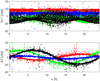 |
Fig. 4 Differences between radio source coordinate estimates (α* = α · cos δ, δ) from three solutions (red, green, and blue dots), applying the NNR condition on three different subgroups of 101 ICRF3 defining sources each and a solution aligned with all 303 ICRF3 defining sources. The black dots are the differences between the VIE2022b-sx solution (301 ICRF3 defining sources) and the solution with all 303 ICRF3 defining sources. |
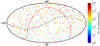 |
Fig. 5 Number of observations of the ICRF3 defining sources from March 27, 2018 (ICRF3 cutoff date), until June 23, 2022 (VIE2022b-sx cutoff date). The black dashed line depicts the ecliptic plane and the red line represents the Galactic plane with the Galactic center denoted as an empty black circle. |
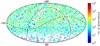 |
Fig. 6 Number of observations of the ICRF3 nondefining sources from March 27, 2018 (ICRF3 cutoff date), until June 23, 2022 (VIE2022b-sx cutoff date). |
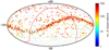 |
Fig. 7 Number of observations of the sources which were observed for the first time after March 27, 2018 (ICRF3 cutoff date) until June 23, 2022 (VIE2022b-sx cutoff date). |
Statistics on observations in VIE2022b-sx from March 27, 2018 (ICRF3 cutoff date), to June 23, 2022 (VIE2022b-sx cutoff date).
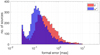 |
Fig. 8 Distribution of source coordinate formal errors in VIE2022b-sx. |
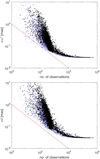 |
Fig. 9 Formal errors in α* (upper plot) and δ (lower plot) with respect to the number of observations in VIE2022b-sx (black dots) and ICRF3 (light blue dots). The red line depicts the hypothetical decrease in formal errors with the square root of the number of observations. |
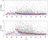 |
Fig. 10 VIE2022b-sx formal errors (gray dots) in α* (upper plot) and δ (lower plot) with respect to declination. Crosses depict median formal errors computed over 2° declination in red for VIE2022b-sx and in blue for ICRF3. |
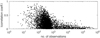 |
Fig. 11 Correlation coefficients between α* and δ with respect to number of observations in VIE2022b-sx. |
VSH parameters up to degree two for VIE2022b-sx minus ICRF3, and VIE2022b-sx minus USNO-2022July03 after eliminating outliers.
List of sources with an angular separation between ICRF3 and VIE2022b-sx of larger than 10 mas.
5 Summary
We present high-precision CRFs and TRFs as provided by the IVS Special Analysis Center VIE. We compare our recent solutions, which include IVS sessions until June 2022 with the current international reference frames, namely ICRF3 and ITRF2020, and highlight the differences coming from the additional VLBI observations after the cutoff dates for the international frames, namely March 2018 and December 2020, respectively. The consistent Vienna CRFs and TRFs are estimated in a common global least squares adjustment and are publicly available together with the corresponding EOPs at the VIE web-page13. In this paper, we provide a detailed description of the underlying a priori models and the selected parametrization for the global least squares solution. We show that our latest VIE2022b solution is superior to ITRF2020 in terms of the estimated positions and velocities of the newest VGOS telescopes, because the observation data available after the ITRF2020 cutoff are crucial for the reliability of position and velocity estimates. The CRF VIE2022b-sx includes the positions of an additional 870 radio sources observed after the ICRF3 cutoff date for the first time. Finally, we show that only 13 of these sources are located in the deep south (declination lower than −45°), which means that special effort to densify the southern sky with more VLBI observations is still desirable.
Acknowledgements
The constructive comments from an anonymous referee are highly appreciated. The authors acknowledge the International VLBI Service for Geodesy and Astrometry (IVS) and all its components for providing VLBI data. J.B. and F.J. would like to thank the Austrian Science Fund (FWF) for supporting their work with project VGOS-Squared (P 31625).
References
- Altamimi, Z., Rebischung, P., Métivier, L., & Collilieux, X. 2016, J. Geophys. Res. Solid Earth, 121, 6109 [NASA ADS] [CrossRef] [Google Scholar]
- Altamimi, Z., Rebischung, P., Collilieux, X., Métivier, L., & Chanard, K. 2022, EGU General Assembly 2022, 3958 [Google Scholar]
- Artz, T., Springer, A., & Nothnagel, A. 2014, J. Geodesy, 88, 1145 [NASA ADS] [CrossRef] [Google Scholar]
- Beasley, A., Gordon, D., Peck, A., et al. 2002, ApJS, 141, 13 [NASA ADS] [CrossRef] [Google Scholar]
- Böhm, J., Werl, B., & Schuh, H. 2006, J. Geophys. Res. Solid Earth, 111, B02406 [Google Scholar]
- Böhm, J., Böhm, S., Boisits, J., et al. 2018, PASP, 130, 044503 [CrossRef] [Google Scholar]
- Brockmann, E. 1997, PhD thesis, Universität Bern, Switzerland [Google Scholar]
- Capitaine, N., Wallace, P. T., & Chapront, J. 2003, A & A, 412, 567 [NASA ADS] [CrossRef] [EDP Sciences] [Google Scholar]
- Charlot, P., Jacobs, C. S., Gordon, D., et al. 2020, A & A, 644, A159 [NASA ADS] [CrossRef] [EDP Sciences] [Google Scholar]
- de Witt, A., Le Bail, K., Jacobs, C., et al. 2019, in IVS GM Proceedings, eds. K. L. Armstrong, K. D. Baver, & D. Behrend (NASA), 189 [Google Scholar]
- de Witt, A., Basu, S., Charlot, P., et al. 2021, in EVGA WM Proceedings, ed. R. Haas, 85 [Google Scholar]
- de Witt, A., Charlot, P., Gordon, D., & Jacobs, C. S. 2022, Universe, 8, 374 [NASA ADS] [CrossRef] [Google Scholar]
- Desai, S. D., & Sibois, A. E. 2016, J. Geophys. Res. Solid Earth, 121, 5237 [NASA ADS] [CrossRef] [Google Scholar]
- Egbert, G. D., & Erofeeva, S. Y. 2002, J. Atmos. Ocean Tech., 19, 183 [NASA ADS] [CrossRef] [Google Scholar]
- Fey, A. L., Gordon, D., Jacobs, C. S., et al. 2015, AJ, 150, 58 [Google Scholar]
- Fomalont, E., Petrov, L. D. S. M., Gordon, D., & Ma, C. 2003, AJ, 126, 2562 [NASA ADS] [CrossRef] [Google Scholar]
- Frey, S., & Titov, O. 2021, Res. Notes AAS, 5, 60 [NASA ADS] [CrossRef] [Google Scholar]
- Gipson, J., & IVS Working Group IV on Data Structures. 2021, 141 [Google Scholar]
- Gipson, J., MacMillan, D., & Petrov, L. 2008, in IVS GM Proceedings, eds. A. Finkelstein, & D. Behrend, 157 [Google Scholar]
- Gordon, D., Jacobs, C., Beasley, A., et al. 2016, AJ, 151, 154 [NASA ADS] [CrossRef] [Google Scholar]
- Hellmers, H., Modiri, S., Bachmann, S., et al. 2022, in International Association of Geodesy Symposia (Springer Berlin Heidelberg), 1 [Google Scholar]
- Iz, H., & Chen, Y. 1999, J. Geodyn., 28, 131 [NASA ADS] [CrossRef] [Google Scholar]
- Jacobs, C., Heflin, M., Lanyi, G., Sovers, O., & Steppe, J. 2010, in IVS GM Proceedings, eds. D. Behrend, & K. D. Baver (NASA), 305 [Google Scholar]
- Kovalev, Y., Petrov, L., Fomalont, E., & Gordon, D. 2007, AJ, 133, 1236 [NASA ADS] [CrossRef] [Google Scholar]
- Krásná, H., Malkin, Z., & Böhm, J. 2015, J. Geodesy, 89, 1019 [CrossRef] [Google Scholar]
- Krásná, H., Jaron, F., Gruber, J., Böhm, J., & Nothnagel, A. 2021, J. Geodesy, 95, 126 [CrossRef] [Google Scholar]
- Landskron, D., & Böhm, J. 2018, J. Geodesy, 92, 349 [NASA ADS] [CrossRef] [Google Scholar]
- MacMillan, D. S., & Ma, C. 1997, Geophys. Res. Lett., 24, 453 [NASA ADS] [CrossRef] [Google Scholar]
- Mathews, P. M., Herring, T. A., & Buffett, B. A. 2002, J. Geophys. Res. Solid Earth, 107, ETG 3 [CrossRef] [Google Scholar]
- Mayer, D., & Böhm, J. 2020, in Beyond 100: The Next Century in Geodesy, eds. J. T. Freymueller, & L. Sánchez (Cham: Springer International Publishing), 21 [CrossRef] [Google Scholar]
- McCallum, L., Wakasugi, T., & Shu, F. 2019, in IVS GM Proceedings, eds. K. L. Armstrong, K. D. Baver, & D. Behrend (NASA/CP-2019-219039), 131 [Google Scholar]
- McCallum, L., Chin Chuan, L., Krásná, H., et al. 2022, J. Geodesy, 96, 1 [CrossRef] [Google Scholar]
- Mignard, F., & Klioner, S. 2012, A & A, 547, A59 [NASA ADS] [CrossRef] [EDP Sciences] [Google Scholar]
- Nothnagel, A. 2009, J. Geodesy, 83, 787 [NASA ADS] [CrossRef] [Google Scholar]
- Nothnagel, A., Artz, T., Behrend, D., & Malkin, Z. 2017, J. Geodesy, 91, 711 [NASA ADS] [CrossRef] [Google Scholar]
- Petit, G., & Luzum, B., eds. 2010, IERS Conventions 2010 (IERS Technical Note No. 36) (Frankfurt am Main: Verlag des Bundesamts für Kartographie und Geodäsie), 179 [Google Scholar]
- Petrachenko, B., Niell, A., Behrend, D., et al. 2009, Design Aspects of the VLBI2010 System. Progress Report of the VLBI2010 Committee, Technical Memorandum NASA/TM-2009-214180 [Google Scholar]
- Petrov, L., Kovalev, Y., Fomalont, E., & Gordon, D. 2005, AJ, 129, 1163 [NASA ADS] [CrossRef] [Google Scholar]
- Petrov, L., Kovalev, Y., Fomalont, E., & Gordon, D. 2006, AJ, 131, 1872 [NASA ADS] [CrossRef] [Google Scholar]
- Petrov, L., Kovalev, Y., Fomalont, E., & Gordon, D. 2008, AJ, 136, 580 [NASA ADS] [CrossRef] [Google Scholar]
- Saastamoinen, J. 1972, Bull. Geodesique, 106, 383 [NASA ADS] [CrossRef] [Google Scholar]
- Tesmer, V., Steigenberger, P., Rothacher, M., Böhm, J., & Meisel, B. 2009, J. Geodesy, 83, 973 [NASA ADS] [CrossRef] [Google Scholar]
- Titov, O., & Lambert, S. 2013, A & A, 559, A95 [CrossRef] [EDP Sciences] [Google Scholar]
- Titov, O., Frey, S., Melnikov, A., et al. 2022, MNRAS, 512, 874 [NASA ADS] [CrossRef] [Google Scholar]
- Weston, S., de Witt, A., Krásná, H., et al. 2023, PASA, 40, e041 [NASA ADS] [CrossRef] [Google Scholar]
- Wijaya, D. D., Böhm, J., Karbon, M., Krásná, H., & Schuh, H. 2013, Atmospheric Effects in Space Geodesy, eds. J. Böhm, & H. Schuh (Springer Berlin Heidelberg), 137 [CrossRef] [Google Scholar]
- Zensus, J., Diamond, P., & Napier, P. 1995, Very Long Baseline Interferometry and the VLBA, ASPC Series, 82 (Astronomical Society of the Pacific) [Google Scholar]
All Tables
Seasonal signal in station height of new VGOS antennas and legacy antennas at common sites.
Statistics on observations in VIE2022b-sx from March 27, 2018 (ICRF3 cutoff date), to June 23, 2022 (VIE2022b-sx cutoff date).
VSH parameters up to degree two for VIE2022b-sx minus ICRF3, and VIE2022b-sx minus USNO-2022July03 after eliminating outliers.
List of sources with an angular separation between ICRF3 and VIE2022b-sx of larger than 10 mas.
All Figures
|
Fig. 1 Antenna participation in VLBI sessions in solution VIE2022b. Red crosses depict the placement of position breaks. Only antennas included in more than 50 sessions are plotted. |
| In the text | |
|
Fig. 2 Annual (blue) and semi-annual (red) height signal in VIE2022b. The amplitude is depicted by the arrow length. The phase of the maximum displacement is represented by the orientation of the arrow. If the arrow points toward north, the maximum appears in January and continues clockwise thereafter. The maximum of the semi-annual signal is depicted in the first half year. |
| In the text | |
|
Fig. 3 Session-wise scale factor computed with VIE2022b parametrization with respect to ITRF2020. The black line represents the smoothed scale factor obtained by local regression using a span of 5% of the total number of data points. |
| In the text | |
|
Fig. 4 Differences between radio source coordinate estimates (α* = α · cos δ, δ) from three solutions (red, green, and blue dots), applying the NNR condition on three different subgroups of 101 ICRF3 defining sources each and a solution aligned with all 303 ICRF3 defining sources. The black dots are the differences between the VIE2022b-sx solution (301 ICRF3 defining sources) and the solution with all 303 ICRF3 defining sources. |
| In the text | |
|
Fig. 5 Number of observations of the ICRF3 defining sources from March 27, 2018 (ICRF3 cutoff date), until June 23, 2022 (VIE2022b-sx cutoff date). The black dashed line depicts the ecliptic plane and the red line represents the Galactic plane with the Galactic center denoted as an empty black circle. |
| In the text | |
|
Fig. 6 Number of observations of the ICRF3 nondefining sources from March 27, 2018 (ICRF3 cutoff date), until June 23, 2022 (VIE2022b-sx cutoff date). |
| In the text | |
|
Fig. 7 Number of observations of the sources which were observed for the first time after March 27, 2018 (ICRF3 cutoff date) until June 23, 2022 (VIE2022b-sx cutoff date). |
| In the text | |
|
Fig. 8 Distribution of source coordinate formal errors in VIE2022b-sx. |
| In the text | |
|
Fig. 9 Formal errors in α* (upper plot) and δ (lower plot) with respect to the number of observations in VIE2022b-sx (black dots) and ICRF3 (light blue dots). The red line depicts the hypothetical decrease in formal errors with the square root of the number of observations. |
| In the text | |
|
Fig. 10 VIE2022b-sx formal errors (gray dots) in α* (upper plot) and δ (lower plot) with respect to declination. Crosses depict median formal errors computed over 2° declination in red for VIE2022b-sx and in blue for ICRF3. |
| In the text | |
|
Fig. 11 Correlation coefficients between α* and δ with respect to number of observations in VIE2022b-sx. |
| In the text | |
Current usage metrics show cumulative count of Article Views (full-text article views including HTML views, PDF and ePub downloads, according to the available data) and Abstracts Views on Vision4Press platform.
Data correspond to usage on the plateform after 2015. The current usage metrics is available 48-96 hours after online publication and is updated daily on week days.
Initial download of the metrics may take a while.