| Issue |
A&A
Volume 678, October 2023
|
|
|---|---|---|
| Article Number | A138 | |
| Number of page(s) | 10 | |
| Section | Stellar atmospheres | |
| DOI | https://doi.org/10.1051/0004-6361/202346853 | |
| Published online | 16 October 2023 | |
Toward more accurate RR Lyrae metallicities★
Konkoly Observatory, Research Center for Astronomy and Earth Sciences, Eötvös Loránd Research Network Budapest,
1121
Konkoly
Thege ut. 15-17, Hungary
e-mail: This email address is being protected from spambots. You need JavaScript enabled to view it.
Received:
9
May
2023
Accepted:
21
August
2023
Abstract
By using a large sample of fundamental mode RR Lyrae stars with published spectroscopic iron abundances and gravities, we point out the importance of correcting these abundances by using more accurate temporal gravities. For the 197 stars with multiple spectra, overall we find [Fe/H] standard deviations of 0.167 (as published), 0.145 (shifted by data source zero points), and 0.121 (both zero point shifted and corrected for the static gravity). These improvements are significant at the ~2σ level at each correction step, leading to a clearly significant improvement after both corrections are applied. The higher quality of the gravity-corrected metallicities is also strongly supported by the tighter correlation with the metallicities predicted from the period and Fourier phase, φ31. This work highlights the need for using some external estimates of the temporal gravity in the chemical abundance analysis, rather than relying on a full-fetched spectrum fit that leads to large correlated errors in the estimated parameters.
Key words: stars: abundances / stars: variables: RR Lyrae / stars: horizontal-branch
Metallicities and light curve parameters used in this paper are available at the CDS via anonymous ftp to cdsarc.cds.unistra.fr (130.79.128.5) or via https://cdsarc.cds.unistra.fr/viz-bin/cat/J/A+A/678/A138
© The Authors 2023
 Open Access article, published by EDP Sciences, under the terms of the Creative Commons Attribution License (https://creativecommons.org/licenses/by/4.0), which permits unrestricted use, distribution, and reproduction in any medium, provided the original work is properly cited.
This article is published in open access under the Subscribe to Open model. This email address is being protected from spambots. You need JavaScript enabled to view it. to support open access publication.
1 Introduction
Heavy elements, that is, primarily [Fe/H], but also α elements, play a leading role in the evolution of RR Lyrae stars as well as in their applicability as distance indicators and tracers of Galactic structure. Unfortunately, they also have highly variable envelopes and atmospheres, making the applicability of standard spectroscopic methods for chemical abundance analysis rather sensitive to the pulsation phase at the moment of observation.
In general, spectroscopic abundances are determined by direct model (alternatively, spectral library or template) fits by adjusting basic atmospheric parameters, such as effective temperature, Teff, temporal gravity, log g, and turbulent velocity, Vt, together with the assumed element distribution (see, e.g., Jofré et al. 2019, for an overview of the methodologies used to produce today’s “industrial” stellar abundances). Unfortunately, this process is beset by rather ill-conditioned and the fitted parameters are both correlated and erroneous. To improve the conditioning, when possible, some of the parameters (usually Teff and log g) are determined externally, by using some reliable parameter source (e.g., spectral energy density fit from multi-waveband observations to derive Teff). The gravity parameter is usually the most difficult parameter to estimate. However, extrasolar planet host stars (or the primary components of binaries with low-mass secondary components) and pulsating variables are excellent candidates for giving good estimates on the temporal value of log g. For extrasolar planet host stars the gravity is well estimated from the combination of the orbital and stellar evolution model analyses (Noyes et al. 2008). For radially pulsating stars, the temporal gravity is very closely estimated from the period (e.g., Gough et al. 1965; Dékány et al. 2008) and from the radial velocity curve (e.g., Clementini et al. 1995).
Considering only RRab (fundamental mode) variables, here we examine the effect of employing a simple post-correction method on the already determined spectroscopic metallicities to improve the accuracy of the final abundances. In addition to the improvement of the internal accuracy, external relations are also used to test the quality of the derived abundances. We refer to the Appendix for additional details of the analysis presented in the paper. Extended materials related to this paper are available at the CDS.
2 Method
The main issue in the derivation of stellar parameters on a purely spectroscopic basis is that in general, these parameters are difficult to disentangle. The success of the process depends on many factors and the verification of the reliability of the parameters derived are often presumptive (e.g., cluster’s chemical homogeneity). For dynamical atmospheres, the situation is coupled with changing stellar atmospheric conditions and physical assumptions, such as the validity of local thermodinamical equilibrium.
Here, we focus on the single problem of temporal gravity. The generally employed spectroscopic element determination methods make this parameter free-floating (together with the iron abundance and Teff; see, e.g., Crestani et al. 2021). However, for classical radial pulsators, we have reliable estimates both for the dynamical part of the gravity (from the radial velocity) and for the static part (from the pulsation equation) as well. Therefore, in principle, we could use a fairly accurate estimate for the temporal value of the gravity and determine only Teff as well as the chemical abundances. Except for Clementini et al. (1995) and Lambert et al. (1996), we could not find any other work following this methodology. Consequently, we have to resort to some method that uses the already published atmospheric parameters and transforms the temporarily given abundances to the value corresponding to the static gravity.
Our approach is purely empirical. After experimenting with various data sets, we found that a linear transformation applied on the published (spectroscopic) [Fe/H] values1 yields more stable [Fe/H] values and, therefore, a supposedly better estimate of [Fe/H]:
![Mathematical equation: $ {\left[ {{{{\rm{Fe}}} \mathord{\left/ {\vphantom {{{\rm{Fe}}} {\rm{H}}}} \right. \kern-\nulldelimiterspace} {\rm{H}}}} \right]_0} = {\left[ {{{{\rm{Fe}}} \mathord{\left/ {\vphantom {{{\rm{Fe}}} {\rm{H}}}} \right. \kern-\nulldelimiterspace} {\rm{H}}}} \right]_{{\rm{sp}}}} + {C_g}\left( {{\rm{log}}\,g - {\rm{log}}\,{g_{{\rm{sp}}}}} \right), $](/articles/aa/full_html/2023/10/aa46853-23/aa46853-23-eq1.png) (1)
(1)
where [Fe/H]0 and [Fe/H]sp, respectively, stand for the transformed and the direct spectroscopic abundances (with the associated static and spectroscopic gravities log g and log gsp). The gravity factor, Cg, is kept constant at the value to be determined by two different criteria (both seem to prefer a value near 0.3; see Sect. 4).
The static log g can be easily obtained from linear stellar pulsation models. Although the single parameter (i.e., period) dependence of the gravity is very strong, the final formula also depends on the parameter coverage of the models. The following formula was derived from the models of Kovacs & Karamiqucham (2021b) covering the RR Lyrae parameter space and combining solar-scaled models with overall heavy element contents of Z = 0.0008 and 0.001:
 (2)
(2)
This formula fits the model logg values with σ = 0.028, appropriate for the purpose of correcting the gravity effect in [Fe/H].
In addition to the gravity effect, different metallicity surveys do not use the very same methodology, including codes, spectral line list, turbulent velocity, temperature scale, solar metallicity, and so on. As a result, there are author- and source-dependent overall zero point (ZP) differences among the different studies. Furthermore, Eq. (1) is intended only to minimize the gravity dependence, but this does not guarantee that the resulting [Fe/H] is also close enough to the static value. To consider both of these effects, we employed source-by-source differential corrections as follows:
![Mathematical equation: $ \left[ {{{{\rm{Fe}}} \mathord{\left/ {\vphantom {{{\rm{Fe}}} {\rm{H}}}} \right. \kern-\nulldelimiterspace} {\rm{H}}}} \right]\left( {\rm{i}} \right) = {\left[ {{{{\rm{Fe}}} \mathord{\left/ {\vphantom {{{\rm{Fe}}} {\rm{H}}}} \right. \kern-\nulldelimiterspace} {\rm{H}}}} \right]_0}\left( {\rm{i}} \right) + {\rm{DZP}}\left( {\rm{i}} \right), $](/articles/aa/full_html/2023/10/aa46853-23/aa46853-23-eq3.png) (3)
(3)
where [Fe/H]0(i) is the gravity-corrected abundance for some star in the ith source. Because the methodology followed by Clementini et al. (1995) and Lambert et al. (1996) seems to be the closest to the type of method we advocate, the DZP-s are determined in a way which considers the averages of all available metallicities, but these are additionally shifted (uniformly) by an amount of −0.08 dex that results the smallest ZP corrections for the metallicities from the above two publications2.
To sum it up, for any fixed Cg, the algorithm of transforming the published spectroscopic abundances to a uniform scale that observes the start-by-star log g and the survey-by-survey ZP dependences, is made up of the following steps:
Gravity correction: use Eqs. (1) and (2) for all stars in all sources.
Estimate the “ridge” by using each star with multiple sources and compute simple averages from the logg-corrected [Fe/H]0 values.
ZP corrections: compute DZP for each source as given by Eq. (3) by considering the average difference between the ridge and the source values. Add −0.08 dex as a global correction to each DZP.
Final [Fe/H]: use Eqs. (1) and (2) again, and derive the final metallicities FEH by employing the gravity correction on the ZP-corrected input [Fe/H]sp values and perform simple averaging for objects with multiple measurements.
The above core scheme is run for the scanned Cg values in the process to be aimed at the optimization of Cg by using various minimization criteria for the root mean square (RMS) of the resulting metallicities (see Sect. 4).
3 Data sets
In gathering high-quality [Fe/H] data, first we made a search for publications with simultaneous Teff and log g data based on high dispersion spectroscopic (HDS) observations. Then, these data were further extended by big survey data (LAMOST and GALAH). Although LAMOST does not use a HDS equipment, the method employed is very similar to those of the HDS small-scale studies. Therefore, for simplicity, we also labeled these data as HDS. The final list of HDS data is based on an additional cross-check of the above big survey databases with the list of Muraveva et al. (2018). We recall that only RRab variables are included in all these and subsequent data sets.
Some details of the HDS inventory used are shown in Table 1. We also checked two more sources: Sprague et al. (2022), based on the APOGEE survey and Gilligan et al. (2021) from the observations made by SALT/HRS. Unfortunately, both of these sets proved to be too noisy with respect of the sources listed in Table 1.
As a consistency check, we also examined the earlier low dispersion spectroscopic (LDS) data by Layden (1994) and Suntzeff et al. (1994), (hereafter, LA94 and SU94, respectively). We recall that the LDS metallicities are based on the calibration of spectral indices (or equivalent widths) that are conveniently measured also on low dispersion spectra. These data are then calibrated on proper sets of [Fe/H] derived from HDS spectra (with the HDS methodology). Once that LDS parameters have been calibrated, they can be quickly applied to determine the metallicities of new objects, often not accessible by HDS instruments. Some-what surprisingly, we found that these early sets follow quite well the HDS ridge (star-by-star average [Fe/H]; see Fig. 1). Both sets show systematic differences with respect to the HDS values. We approximate these trends by straight lines. The regression coefficients are given in Table 2. The improved quality of the merged (HDS & LDS) data will be demonstrated in Sect. 5.
Concerning the calibration of the gravity- and source ZP-corrected [Fe/H] relative to the Sun, we note that an overwhelming majority of the sources use log ϵ(Fe) = 7.50. Therefore, [Fe/H] presented in this work is considered to be tied to this solar value.
4 The gravity factor
Before dwelling more deeply into the gravity correction, it is worth examining the distribution of the published gravities of the various surveys and targeted studies. Figure 2 shows the distribution of the gravity differences Δ log g = log g − log gsp for the various sources. Large deviations can be seen in both directions, suggesting improper pulsation phasing of the observations, or, more likely, large errors in the spectroscopic gravities. The surprisingly flat pattern of log g for the set of fo11 (For et al. 2011) is due to their specific sample of stars, with periods concentrated in a narrow range. The striking linear dependence for fe96, fe97, and so96 (respectively, Fernley & Barnes 1996, 1997; Solano et al. 1997) is due to the fixed log gsp values in their analysis. The Δ log g ranges are particular small and quite close to the values predicted by Eq. (2) for la96 and cl95 (Lambert et al. 1996; Clementini et al. 1995), respectively, indicating a proper phasing of the observations in these studies.
After a detailed examination of the star-by-star dependence of the published [Fe/H] values on gravity difference log g − log gsp, we found that the gravity factor Cg (Eq. (1)) has a visible target dependence. For instance, Z Mic has remarkably constant [Fe/H] implying Cg ~ 0.0, whereas V1645 Sgr is best fitted by a steep Cg of ~0.6. However, using individual Cg would lead to a high level of overfitting, due to the modest number of spectra for most of the stars3. Therefore, we decided to search for the best global value of Cg, by minimizing the scatter of the log g-transformed and source ZP-adjusted abundances around the average values for all stars with multiple spectra (197 stars and 1037 spectra altogether). Black dots in Fig. 3 show the run of RMS (individual transformed metallicities {feh} minus their average FEH) for the full scan range of Cg. A preference for Cg ~ 0.2 is clearly visible.
Yet another way to optimize Cg, is to scan the dependence of the RMS of the (P, φ31) → FEH fit (Jurcsik & Kovacs 1996), this time using the full HDS set, including single spectra data (263 objects with available V light curves – see Sect. 5). Gray dots in Fig. 3 indicate a preference of high significance for a global value of Cg ~ 0.3.
To further constrain Cg, we also attempted to test the tightness of the [Fe/H]−MV (e.g., Castellani et al. 1991) and the near infrared period-luminosity-metallicity (PLZ, i.e., Bono et al. 2003) relations. Unfortunately, both of these relations have relatively weak metal dependences. In addition, this dependence is further masked by noise, internal physical scatter (for the [Fe/H]−MV relation) and the correlation between the period and metallicity (for the PLZ test). Therefore, we relied only on the direct tests shown in Fig. 3. These tests suggest values of Cg ~ 0.25, which we will use throughout the paper.
For a very simple demonstration of the differential log g-dependence of the published spectroscopic abundances, in Fig. 4 we plot these [Fe/H] values as a function of Δ log g = log g − log gsp (with log g as given by Eq. (2)). In the left panel, all [Fe/H] were taken straight from the respective publications and plotted against Δ log g. In the right panel we employed source ZP corrections as described in Sect. 2 and presented in Table 1. For each star, the [Fe/H]sp values were fitted by a straight line of Eq. (1) with Cg = 0.25 and [Fe/H]0 adjusted by a least-squares fit of equal weights.
As noted earlier, although in most cases the adopted slope is in good agreement with the observations, there are cases with considerable differences (steeper, e.g., V1645 Sgr and shallower, such as AN Ser). Source ZP corrections further improve the fit as can be seen by the insets at each object showing the RMS of the residuals around the straight lines.
We can also visualize the Δ log g →[Fe/H] correlation by collapsing the data in the vertical axis (i.e., not applying star-by-star vertical shifts). The left panel of Fig. 5 shows the result of this type of data handling by using the full sample of 197 stars with multiple measurements. In the right panel, in addition to showing two well-fit cases we also exhibit the specific data from Lambert et al. (1996). To the best of our knowledge their work is the only one (in the context of RR Lyrae stars) comparing metallicities from the traditional spectroscopic method and those obtained by using known values of the temporal gravity and theoretical spectral models.
Using Table 3 of Lambert et al. (1996), first we calculated the average of the “photometric” metallicities derived from the FeI and FeII lines4. These metallicities were obtained by employing the log g values mostly from various Baade-Wesselink analyses, and, in fewer cases, from narrow-band photometry. Then, we used the “spectroscopic” metallicities5 to calculate the difference between these and the “photometric” metallicities. The corresponding gravity differences (“spectroscopic” minus “photometric”) are also listed in the same table of Lambert et al. (1996). Except for a vertical adjustment of −0.09 dex, we plotted these published values in Fig. 5 straight. The 15 RRab stars follow the trend observed by the other two individual objects with multiple measurements remarkably well.
Although there might exist several contributing factors to the correlation between Δ log g and [Fe/H], non-LTE effects are likely play a leading role (Lambert et al. 1996). The work by Luck & Lambert (1985) on intermediate-mass supergiants (including Cepheids) was the first to point out the systematic differences between the gravities obtained from the spectroscopic analyses and pulsation models. Being less sensitive to non-LTE effects, Kovtyukh & Andrievsky (1999) suggest using Fe II lines for abundance and gravity estimates in the case of Cepheids. Lambert et al. (1996) lend on a similar conclusion for RR Lyrae stars. For yet another support of the generality of the role non-LTE effects in establishing the correlation between log g and [Fe/H], we refer to the work of Thévenin & Idiart (1999) on late-type non-variable stars.
To visualize the improvement of the quality of the derived metallicities at various stages of the process, in Fig. 6, we show the star-by-star standard deviations for the above set of 197 stars. The ZP correction yield an RMS improvement which is significant at the 2σ level. This is quite close to the additional 2.3 sigma significance of the gravity correction on the ZP-corrected values. All these indicate essentially the same level of importance of both types of correction.
HDS inventory.
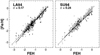 |
Fig. 1 HDS ridge metallicities (FEH) vs individual HDS (gray dots) and LDS (black dots) metallicities. The corresponding regression lines are shown by gray and black lines. The standard deviations of the LDS regressions are shown in the upper left corners of the corresponding LDS sources: LA94 for Layden (1994) and SU94 for Suntzeff et al. (1994). |
LDS to HDS transformations.
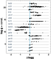 |
Fig. 2 Gravity differences (static value – log g, from Eq. (2) – minus published spectroscopic value) for the individual objects of the different sources. For each source, a uniform vertical shift was applied to separate it from the data of other sources. See Table 1 for the source acronyms. |
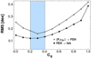 |
Fig. 3 Dependence of the fit RMS values on the gravity correction factor Cg (see Eq. (1)). The plot shows the scans resulting from the direct estimates of the scatter of the individual transformed abundances {feh} around the average values {FEH} and the variation of the fit RMS of the Fourier-based estimates. The shaded box indicates the optimum regime for Cg. |
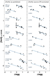 |
Fig. 4 Examples of the star-by-star correlation between the gravity difference and the published abundances (left panel). The same correlation is shown in the right panel after source ZP corrections. For an easier visualization, vertical shifts were applied together with a factor of two decrease of the [Fe/H] ranges (including the slope of the fitted straight line with an original value of −0.25). Numbers at the individual objects show the RMS values around the straight lines). See text for further details. |
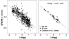 |
Fig. 5 Correlation between the published HDS metallicities and the difference between the static and spectroscopic gravities. Left: correlation for the 197 stars with multiple spectra. To avoid scatter due to differences in the individual stellar metallicities, star-by-star vertical shifts were applied by using the average metallicities after gravity correction (see Eq. (1)). Right: same as in the left panel, but only for two well-fit examples. We also plot the RRab sample from Table 3 of Lambert et al. (1996) by using the “photometric” and “spectroscopic” results (see text for further details). |
5 The (P,φ31) → [Fe/H] fit
Here, we further test the gravity- and source zero point-corrected metallicities FEH (Sects. 4 and 3). This test also casts more light on the potentials and limitations of the metallicity determination based on light curve analyses (Kovacs & Zsoldos 1995; Jurcsik & Kovacs 1996). Unfortunately, this relation still remains to be purely empirical, without any theoretical foundation (except perhaps for the work of Feuchtinger 1999), in spite of the practical applicability and current recalibrations on various data sets (e.g., Dékány & Grebel 2022; Li et al. 2023)6.
We use the light curves from the ASAS and ASAS-SN surveys (Pojmanski 1997; Shappee et al. 2014; Christy et al. 2023) and the Fourier decompositions presented by Jurcsik & Kovacs (1996). Because our approach here is to utilize as many spectroscopic [Fe/H] as possible, we included all RRab stars, irrespective of whether they are monomode or Blazhko. If the target is of this latter type, it is frequency analyzed, and the mid curve (i.e., that part of the light curve that comes from the monomode pulsation) is used to estimate the Fourier phase. Additional details of the light curve analysis can be found in Appendix B.
The metallicity data sets to be dealt with are listed in Table 3. These sets were selected to investigate: (i) effect of merging LDS and HDS data to aim for more accurate test base (set A, containing stars with average metallicities derived from HDS and LDS sources); (ii) more realistic situations, when the data quality strongly changes within the sample (set B, with mixed items containing only either HDS or LDS, or type A metallicities). The RMS values indeed show that the merged data yield better result. Assuming Gaussian distributions for the residuals (an assumption that has only partial validity – see later), we get that the RMS differences with respect to set A for AHDS, ALDS, and B are significant at the 1.7, 2.5 and 1.4 sigma levels, respectively. For set AHDS, employing only HDS source ZP corrections (i.e., no gravity correction), we get a fit with an RMS of 0.256. With respect to set A, this increase is significant at the level of 5.7 sigma.
The corresponding regressions for sets A and B are shown in Fig. 7. We recall that the samples shown include all stars (i.e., even those indicated as “clipped” objects in Table 3. Systematically high-fit objects at the low metallicity end are clearly visible. Assuming that the Fourier method is sensitive to the global metallicity [M/H] rather than to [Fe/H], then this effect may come from the stronger α element enhancements at lower metallicities. On the other hand, we see also systematically low-fit values for quite a large number of stars in the mid- to high-metallicity part. A brief test of the effect of possible low (or perhaps negative) α enhancement for these stars by using the estimates of Crestani et al. (2021) did not suggest any statistically significant improvement. A more detailed examination of these stars vaguely implicated that the underestimation by the Fourier method may be partially attributed to the slight excess of Blazhko stars (however, we do not have an explanation why these stars may cause such an effect).
In addition to the visual inspection of the residuals, we can also examine their distribution. It turns out (see Appendix D) that none of the data sets follow Gaussian distribution in the outskirt of their ordered residuals. About 20% of the stars in each sample belong to a non-Gaussian subset. Although several outliers can be explained by light curve or metallicity errors or peculiarities, both in the non-Gaussian set and among the simple outliers as well, there are stars with excellent metallicities and accurate light curves. Stars such as X Ari, AL CMi, or V0341 Aql remain among the puzzling examples related to the use of the Fourier method for [Fe/H] determinations.
From a purely practical point of view, a large fraction of the observed [Fe/H] values can be fitted remarkably well with (P,φ31). The errors are less than 0.2 dex for over 70% and less than 0.1 dex for about 50% of the stars in our samples. Finally, for V light curves (using the monomode components for Blazhko stars), the updated formula derived from set A of Table 3 is expressed as follows7,
 (4)
(4)
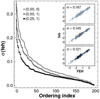 |
Fig. 6 Ordered standard deviations of the multiple [Fe/H] values under various data handling as given by the code list in the upper left part of the figure. First number in the code symbol corresponds to the log g correction term (Cg in Eq. (1)), whereas the second number indicates if source-by-source zero point correction was (1) or was not (0) employed. The inserted panels show the scatter of the star-by-star individual metallicity values {feh} around the corresponding average metallicities FEH. The equality lines are indicated by light blue. The standard deviations are shown by the internal labels. |
Datasets for the (P, φ31) →[Fe/H] test.
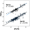 |
Fig. 7 Metallicity predictions FEH31 from the period and Fourier parameter φ31. Datasets given in Table 3 are used including both log g-and ZP-corrected HDS data and LDS data as discussed in Appendix A. These metallicities are shown on the horizontal axis. Straight lines indicate the equality values for [Fe/H]. The plot for set B has been shifted downward for better visibility. |
6 Conclusions
By using the best available iron abundances based on traditional spectral analyses of fundamental mode RR Lyrae stars, we have drawn the following conclusions.
Current spectroscopic abundances suffer from considerable scatter both internally (within a given survey) and externally (between the different surveys).
The internal scatter can be mitigated on a star-by-star basis by employing a linear correction including the difference between the static and the temporal (spectroscopic) gravities.
The external (zero point) differences can be eliminated by uniform survey-by-survey shifts based on the common stars in the different surveys.
Both corrections yield roughly the same degree of improvement in the overall quality of the final abundances, resulting in a RMS of 0.12 dex around the averages for stars with multiple measurements. This is an improvement of more than 4 sigma with respect to the RMS of 0.17 dex of the published (uncorrected) values.
The relatively large differences among the spectroscopic abundances have led us to examine the possible utilization of the metallicity estimates based on spectral index methods (Layden 1994; Suntzeff et al. 1994). Interestingly, we found these metallicities rather comparable with the overall higher accuracy direct spectroscopic metallicities. The merged set of 187 stars (set A in Table 3) represents the most accurate metallicities used in this paper.
The higher quality [Fe/H] also has an influence on the tightness of the relations involving [Fe/H]. Although the effect is rather mild on the [Fe/H]→ MV and near infrared (log P, [Fe/H]) → MKs relations, the improvement on the (P, φ31) →[Fe/H] fit is far more significant. In this update we extended the applicability of the Fourier method to Blazhko stars by using the average light curves, as derived from the Fourier fits including also the Blazhko modulation. The precision of the [Fe/H] estimates are, respectively, within 0.2 and 0.1 dex for some 70 and 50% of the samples investigated. The Fourier-based [Fe/H] yield a little tighter correlations for the above luminosity relations. At the same time, we found puzzling differences between the Fourier estimates and the observed values in several stars. We cannot offer any explanation for this phenomenon at this moment, except perhaps for the vague notion that the Fourier estimate refers more likely to the overall metal abundance rather than [Fe/H] – and that for some reasons some of the stars are α element deficient (rather than enhanced).
Based on the improvement presented in this paper, we strongly argue for the reexamination of methodology of element abundance determination in RR Lyrae stars, as well as pulsating stars, in general. The methods used by Clementini et al. (1995) and Lambert et al. (1996) serve as important examples for the path we think would be very fruitful to pursue.
An early reference to the existence of such a relation can be found in Lambert et al. (1996). See Sect. 4 for further discussion of their result in the context of this paper.
Even though these two publications are based on very close principles, the resulting abundances for the three common stars differ by 0.1–0.2 dex. This paper uses the average of the Fe I and Fe II values in the “photometric” section of Table 3 from Lambert et al. (1996) and Table 12 of Clementini et al. (1995).
Nevertheless, for further support of our adopted value of Cg, it is useful to examine the distribution of the star-by-star fitted Cg values and check the degree of spread of these values. See Appendix C for this test.
Although the correlation with A log g is tighter for FeII (Lambert et al. 1996), we used the average for consistency with the final data set of this paper.
These are derived from direct theoretical spectrum fits, based on equating the abundances obtained from spectral lines of various ionization levels. The gravity is computed as part of the fitting process.
At the same time, it is worthwhile to note that the large datasets used in this paper further strengthen the strong preference for the (P, φ31) dependence against any other two-parameter combinations, including φ41 and Atot (depending on the data sets, at the 1–4 and 8–12σ levels, respectively).
By using set B we get FEH31 = −4.845 − 5.385 P + 1.274 φ31, yielding estimates that deviate from the values predicted by Eq. (4) with a standard deviation of 0.017 dex.
Acknowledgements
We appreciate the discussion with Giuliana Fiorentio on the intricacy of α-enhancement. It is a pleasure to thank the useful comments by Jayasinghe A. Tharindu on the compatibility of the ASAS and ASAS-SN light curves. We thank the referee for drawing our attention on some earlier works relevant for this paper. This research has made use of the VizieR catalogue access tool, CDS, Strasbourg, France (DOI: 10.26093/cds/vizier). This work has made use of data from the European Space Agency (ESA) mission Gaia (https://www.cosmos.esa.int/gaia), processed by the Gaia Data Processing and Analysis Consortium (DPAC, https://www.cosmos.esa.int/web/gaia/dpac/consortium). Funding for the DPAC has been provided by national institutions, in particular the institutions participating in the Gaia Multilateral Agreement. This research has made use of the NASA/IPAC Infrared Science Archive, which is funded by the National Aeronautics and Space Administration and operated by the California Institute of Technology. This research has made use of the International Variable Star Index (VSX) database, operated at AAVSO, Cambridge, Massachusetts, USA. Guoshoujing Telescope (the Large Sky Area Multi-Object Fiber Spectroscopic Telescope LAMOST) is a National Major Scientific Project built by the Chinese Academy of Sciences. Funding for the project has been provided by the National Development and Reform Commission. LAMOST is operated and managed by the National Astronomical Observatories, Chinese Academy of Sciences. This work made use of the Third Data Release of the GALAH Survey (Buder et al. 2021). Supports from the National Research, Development and Innovation Office (grants K 129249 and NN 129075) are acknowledged.
Appendix A Metallicities
Spectroscopic [Fe/H] abundances based on HDS methodology were collected in a multistep process, whereby the additional data sets were iteratively examined for quality control. This process has led to re-instating sources that were priorly excluded and vice verse. Unfortunately, we had to exclude two sources (Gilligan et al. 2021; Sprague et al. 2022) due to excessive scatter around the [Fe/H] ridge established by the other sources. Examples on a well-fit subset and one of the excluded sets are shown in Fig. A.1. Finally, the set of 17 sources was established, with 1279 individual observations, including multiple visits to the same objects. Among the targets there were many RRc stars, several RRd, BL Her and binary stars. These, together with faint (V ≳ 15 mag) objects (of any type) were excluded (altogether 104 objects) from further analysis. The final inventory of 269 RRab stars is shown in Table 1.
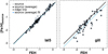 |
Fig. A.1 Source-dependent individual vs ridge metallicities (FEH, averages computed from all sources). Black line shows the ridge, blue line shows the fit to the particular source averages (assuming only a constant shift relative to the ridge line for a given source). Black dots are for the average metallicities, pale, larger circles are for the individual metallicities. The left and right panels show, respectively, the well-fit case of Luo et al. (in prep.) (LAMOST DR5) and the poor-fit case of Gilligan et al. (2021). The latter is not included in our final HDS sample. Table 1 gives the list of the HDS sources. |
Concerning the data handling, the following points worth mentioning. For the “big survey” data (LAMOST and GALAH) an upper error limit of 0.4 dex was employed. After a considerable amount of testing, we decided to use simple averaging instead of robust averaging for the computation of the final metallicities for objects with multiple sources. This choice was justified because of the overall moderate number of multiple measurements for the individual objects. In merging the HDS and LDS data we considered the individual measurements in both sets to be equal, therefore, the final [Fe/H] was computed as a weighted average, namely, [Fe/H]= w[Fe/H]HDS + ((1 − w)[Fe/H]LDS, where w = NHDS/(NHDS + NLDS), and the N-s stand for the number of spectra. Except for the following two stars, all objects were treated equally. We did not use the HDS values of V0455 Oph, because there were differences up to 0.9 dex among the four published values. For WW Vir, the value of Xiang et al. (2019) was an extreme outlier with respect of the values of Luo et al. (in prep.) and Layden (1994), so, Xiang’s et al. value was omitted.
Appendix B Light curves
We opted to employ the long-term V-band time series photometry supplied by the ASAS and ASAS-SN surveys. These projects yield unique data sets fitting perfectly to our goals to derive: (i) reliable low-order phases for testing the Fourier-based [Fe/H] estimation; (ii) homogeneous sets of V magnitude averages for testing the MV dependence on [Fe/H]; (iii) proper decomposition of the light curves into the monomode and Blazhko components for goal (i) and for the assessment of the role of Blazhko phenomenon in the applications.
For variables without an apparent Blazhko modulation, we employed standard least squares Fourier fit up to order 15 (depending on the quality of the light curve). Outliers were iteratively clipped. For the Blazhko stars, first we performed a scan of the Blazhko period by using the following simple Fourier model, considering only the first order modulation side lobes
 (B.1)
(B.1)
where m is the highest harmonics with side lobe frequencies  and
and  . The Blazhko frequency is
  , with ωi being the ith harmonics of the fundamental frequency. We used m = 7 in nearly all cases and constrained the monomode component to order k ≥ m. Although the frequency spectra of Blazhko stars are, in general, more complicated than the simple model above, in a large majority of cases it yielded a good description of the data.
For the Fourier phases and average magnitudes, in addition to ASAS and ASAS-SN, we considered also the data collected by Jurcsik & Kovacs (1996) based on classical individual stellar studies. The final set of φ31 and the magnitude averages (V), result from the zero point shifted equal-weighted averages from all possible sources (by equal weighting all three sources). The zero point shifts – Jurcsik & Kovacs (1996) minus the source – for φ31 are −0.015 and +0.015 for ASAS and ASAS-SN, respectively. The shifts for (V) − in the same order and same sense – are as follows: +0.016 and +0.039 mag, with high respective standard deviations of0.013 and 0.037.
There are two stars that have not been used in any light curve-related tests. The brightBlazhko stars RRLyrandXZ Cyg are only in the ASAS-SN database, but they are saturated, with XZ Cyg having too few data points. TZ Aur is monoperiodic, but older data were fractional, resulting questionable Fourier phases. Therefore, the star was not used from Jurcsik & Kovacs (1996).
Appendix C Distribution of the gravity coefficient
As noted in Sect. 4, individual cases might yield quite different values for the gravity factor Cg. To get an overall view on the statistics of the Cg values, for each star, we fit the published [Fe/H] values by an equal-weighted least squares method using the following formula:
![Mathematical equation: $ {\left[ {{{{\rm{Fe}}} \mathord{\left/ {\vphantom {{{\rm{Fe}}} {\rm{H}}}} \right. \kern-\nulldelimiterspace} {\rm{H}}}} \right]_{{\rm{sp}}}} = {a_0} + {a_1}{\rm{\Delta }}\,{\rm{log}}\,g, $](/articles/aa/full_html/2023/10/aa46853-23/aa46853-23-eq10.png) (C.1)
(C.1)
where Δ log g = log g – log gsp, with log g denoting the estimated static (Eq. 2) and log gsp the published spectroscopic gravities. In this equation coefficient a1 corresponds to the object-dependent Cg (with a negative sign, due to the re-arrengement of Eq. 1). The distribution of {a1} is shown in Fig. C.1. We see that the distribution is asymmetric around the zero slope and peaks close to our adopted value of a1 = −0.25. The plot shown was derived
Average gravity coefficient as a function of minimum number of spectra
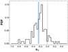 |
Fig. C.1 Probability distribution function of the gravity coefficient, a1, in the linear regression of Δ log g to the published abundances (see Eq. C.1). For reference, dotted and thick vertical lines, respectively, show the a1 = 0.0 and our final adopted value a1 = −0.25. |
Appendix D Associated results
Here, we briefly summarize some of the consequences of the metallicity scale introduced in this paper. We focus on the residual distribution of the metallicity estimate based on the Fourier parameters, the classical metallicity–absolute V magnitude and the near infrared PLZ relations.
A general property of all metallicity sets studied in this paper is the non-Gaussian distribution of the subsets of stars lying in the gray zone of few sigma deviations with respect to the best linear fit of [Fe/H]~ a0 + a1 P + a2φ31. To demonstrate the size of the effect, we used set A of Table 3 (see also Fig. 7 and Eq. 4 for the regression). The ordered residuals are shown in Fig. D.1. For some 80% of the sample, the distribution is within the 3σ range of the same size of sets following Gaussian distribution with a standard deviation of σG = 0.140.
As mentioned in Sect. 5, currently we have no explanation for this phenomenon. Once the outliers (both the non-fitting and non-Gaussian members – 14 stars) are omitted, the resulting sample of 173 stars yields a fit RMS of 0.135 dex and a core Gaussian distribution with σG = 0.127 dex. It is important to recall, that while some stars are suspect of light curve anomalies (e.g., IU Car [period and light curve changes], SS CVn [Blazhko with peculiar average light curve]) several stars, qualified as outliers (e.g., AL CMi, XAri)have very accurate observed abundances, and no apparent light curve anomalies over several (up to many) decades.
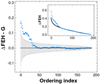 |
Fig. D.1 Testing the (P, φ31) → FEH fit residuals. Inset: Ordered distribution (light blue) of the residuals (ΔFEH = |FEHobs – FEHfit|) for set A of Table 3. Black line shows the distribution of the corresponding Gaussian, fitting the core of the observed residuals. Main panel: Difference between the observed and the predicted Gaussian residuals. The 3σ ranges for the Gaussian residuals are shown by the vertical error bars. |
The effect of the type of metallicity used in studying the metallicity-absolute magnitude relation is shown in Fig. D.2. We used the Gaia DR3 parallaxes (Lindegren et al. 2021) and reddenings by Schlafly & Finkbeiner (2011). Set B of Table 3 was selected as a test base, but we employed cutoffs for E(B – V) and for the relative parallax errors of 0.2 and 0.06, respectively. This had led to a sample of 264 stars. To calculate the Fourier FEH, we used Eq. 4. This yielded a residual standard deviation of 0.163 mag (vs 0.184 from the fit using direct FEH values). The difference is marginally significant (at the 2σ level). By using other samples, we lend on similar conclusions, often with a lower significance. As expected, the linear regressions are also very similar, yielding MV = 1.059 + 0.341 × FEH for the direct and MV = 1.095 + 0.372 × FEH31 for the Fourier-based FEH31. We also examined the effect of gravity and source ZP corrections, and found similar low-significance preference for the corrected metallicities with respect to the uncorrected ones.
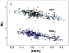 |
Fig. D.2 Iron abundance versus V absolute magnitude, using a subset of set B(see Table 3 and text forthe selection ofthis subset). Lines are the resulting linear regressions. For better visibility, the set using Fourier-based abundances (FEH31) has been shifted downward by 2 mag with respect of the set using the mixture of gravity and source ZP-corrected HDS and LDS metallicities. |
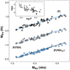 |
Fig. D.3 Observed 2MASS absolute magnitude (Ks) vs predicted magnitudes from various PLZ relations. The lines show the identity values, the labels indicate the formula type used in deriving the various fits. The inset shows the correlation between the two quantities fitted to the Ks magnitudes. See text for sample selection. |
Finally, in Fig. D.3 we show the PL and PLZ relations in the near infrared. The goal of this test is to check: (a) the dependence on the metallicity used; (b) the significance of the metallicity dependence. We use the sample of ~ 100 stars with approximate average Ks magnitudes transformed from the unWISE fluxes (Schlafly et al. 2019) as given by Kovacs & Karamiqucham (2021a). After cross-matching with set B of Table 3 and applying E(B – V) and relative parallax error cuts of 0.5 and 0.03, respectively, we ended up with a sample of 55 stars. As shown in Fig. D.3, we get increasingly better regressions from the single-parameter (log P) fit to those utilizing the metallicities FEH and FEH31. The latter (best) fit is significantly better than the single-parameter fit nearly at the level of 3σ. On the other hand, we found basically no difference between using the original (published, not corrected) [Fe/H] and the gravity/source-corrected FEH. As shown in the inset of Fig. D.3, this is most probably attributed to the significant correlation between log P and [Fe/H] (the period dependence “takes over” if the available [Fe/H] becomes more noisy, yielding a fit of similar quality). Indeed, we obtained the following regressions:
MKs = −1.4316 – 3.6331 × log P,
MKs = −0.9526 – 2.5676 × log P + 0.1554 × FEH,
MKs = −0.8874 – 2.4436 × log P + 0.1899 × FEH31,
with σfit = 0.090, 0.067 and 0.060, respectively.
References
- Andrievsky, S., Wallerstein, G., Korotin, S., et al. 2018, PASP, 130, 4201 [Google Scholar]
- Andrievsky, S. M., Korotin, S. A., Kovtyukh, V. V., et al. 2021, Astron. Nachr., 342, 887 [NASA ADS] [CrossRef] [Google Scholar]
- Bono, G., Caputo, F., Castellani, V., et al. 2003, MNRAS, 344, 1097 [Google Scholar]
- Buder, S., Sharma, S., Kos, J., et al. 2021, MNRAS, 506, 150 [NASA ADS] [CrossRef] [Google Scholar]
- Castellani, V., Chieffi, A., & Pulone, L. 1991, ApJS, 76, 911 [NASA ADS] [CrossRef] [Google Scholar]
- Chadid, M., Sneden, C., & Preston, G. W. 2017, ApJ, 835, 187 [Google Scholar]
- Christy, C. T., Jayasinghe, T., Stanek, K. Z., et al. 2023, MNRAS, 519, 5271 [Google Scholar]
- Clementini, G., Carretta, E., Gratton, R., et al. 1995, AJ, 110, 2319 [Google Scholar]
- Crestani, J., Braga, V. F., Fabrizio, M., et al. 2021, ApJ, 914, 10 [NASA ADS] [CrossRef] [Google Scholar]
- Dékány, I., & Grebel, E. K. 2022, ApJS, 261, 33 [CrossRef] [Google Scholar]
- Dékány, I., Kovacs, G., Jurcsik, J., et al. 2008 MNRAS, 386, 521 [Google Scholar]
- Fernley, J., & Barnes, T. G. 1996, A & A, 312, 957 [NASA ADS] [Google Scholar]
- Fernley, J., & Barnes, T. G. 1997, A & AS, 125, 313 [NASA ADS] [Google Scholar]
- Feuchtinger, M. U. 1999, A & A, 351, 103 [NASA ADS] [Google Scholar]
- For, Bi-Qing, Sneden, C., & Preston, G. W. 2011, ApJS, 197, 29 [NASA ADS] [CrossRef] [Google Scholar]
- Gilligan, C. K., Chaboyer, B., Marengo, M., et al. 2021, MNRAS, 503, 4719 [Google Scholar]
- Gough, D. O., Ostriker, J. P., & Stobie, R. S. 1965, ApJ, 142, 1649 [NASA ADS] [CrossRef] [Google Scholar]
- Jofré, P., Heiter, U., & Soubiran, C. 2019, ARA & A, 57, 571 [CrossRef] [Google Scholar]
- Jurcsik, J., & Kovacs 1996, A & A, 312, 111 [NASA ADS] [Google Scholar]
- Kovacs, G., & Zsoldos, E. 1995, A & A, 293, L57 [NASA ADS] [Google Scholar]
- Kovacs, G., & Karamiqucham, B. 2021a, A & A, 653, A61 [NASA ADS] [CrossRef] [EDP Sciences] [Google Scholar]
- Kovacs, G., & Karamiqucham, B. 2021b, A & A, 654, L4 [NASA ADS] [CrossRef] [EDP Sciences] [Google Scholar]
- Kovtyukh, V. V., & Andrievsky, S. M. 1999, A & A, 351, 597 [NASA ADS] [Google Scholar]
- Lambert, D. L., Heath, J. E., Lemke, M., et al. 1996, ApJS, 103, 183 [NASA ADS] [CrossRef] [Google Scholar]
- Layden, A. C. 1994, AJ, 108, 1016 [Google Scholar]
- Li, X.-Y., Huang, Y., Liu, G.-C., et al. 2023, ApJ, 944, 88 [NASA ADS] [CrossRef] [Google Scholar]
- Lindegren, L., Klioner, S. A., Hernández, J., et al. 2021, A & A, 649, A2 [NASA ADS] [CrossRef] [EDP Sciences] [Google Scholar]
- Liu, S., Zhao, G., Chen, Y.-Q., et al. 2013, RAA, 13, 1307 [NASA ADS] [Google Scholar]
- Luck, R. E., & Lambert, D. L. 1985, ApJ, 298, L782 [NASA ADS] [CrossRef] [Google Scholar]
- Muraveva, T., Delgado, H. E., & Clementini, G., et al. 2018, MNRAS, 481, 1195 [CrossRef] [Google Scholar]
- Nemec, J. M., Cohen, J. G., Ripepi, V., et al. 2013, ApJ, 773, 181 [CrossRef] [Google Scholar]
- Noyes, R. W., Bakos, G. Á., Torres, G., et al. 2008, ApJ, 673, L79 [NASA ADS] [CrossRef] [Google Scholar]
- Pancino, E., Britavskiy, N., Romano, D., et al. 2015, MNRAS, 447, 2404 [Google Scholar]
- Pojmanski, G. 1997, A & A, 47, 467 [NASA ADS] [Google Scholar]
- Schlafly, E. F., & Finkbeiner, D. P. 2011, ApJ, 737, 103 [Google Scholar]
- Schlafly, E. F., Meisner, A. M., & Green, G. M. 2019, ApJS, 240, 30 [Google Scholar]
- Shappee, B. J., Prieto, J. L., Grupe, D., et al. 2014, ApJ, 788, 48 [Google Scholar]
- Solano, E., Garrido, R., Fernley, J., & Barnes, T. G. 1997, A & AS, 125, 321 [NASA ADS] [Google Scholar]
- Sprague, D., Culhane, C., Kounkel, M., et al. 2022, AJ, 163, 152 [NASA ADS] [CrossRef] [Google Scholar]
- Suntzeff, N. B., Kraft, R. P., & Kinman, T. D. 1994, ApJS, 93, 271 [NASA ADS] [CrossRef] [Google Scholar]
- Takeda, Y. 2022, MNRAS, 514, 2450 [CrossRef] [Google Scholar]
- Thévenin, F., & Idiart, T. P. 1999, AJ, 521, 753 [CrossRef] [Google Scholar]
- Xiang, M., Ting, Y.-S., Rix, H.-W., et al. 2019, ApJS, 245, 34 [Google Scholar]
All Tables
All Figures
|
Fig. 1 HDS ridge metallicities (FEH) vs individual HDS (gray dots) and LDS (black dots) metallicities. The corresponding regression lines are shown by gray and black lines. The standard deviations of the LDS regressions are shown in the upper left corners of the corresponding LDS sources: LA94 for Layden (1994) and SU94 for Suntzeff et al. (1994). |
| In the text | |
|
Fig. 2 Gravity differences (static value – log g, from Eq. (2) – minus published spectroscopic value) for the individual objects of the different sources. For each source, a uniform vertical shift was applied to separate it from the data of other sources. See Table 1 for the source acronyms. |
| In the text | |
|
Fig. 3 Dependence of the fit RMS values on the gravity correction factor Cg (see Eq. (1)). The plot shows the scans resulting from the direct estimates of the scatter of the individual transformed abundances {feh} around the average values {FEH} and the variation of the fit RMS of the Fourier-based estimates. The shaded box indicates the optimum regime for Cg. |
| In the text | |
|
Fig. 4 Examples of the star-by-star correlation between the gravity difference and the published abundances (left panel). The same correlation is shown in the right panel after source ZP corrections. For an easier visualization, vertical shifts were applied together with a factor of two decrease of the [Fe/H] ranges (including the slope of the fitted straight line with an original value of −0.25). Numbers at the individual objects show the RMS values around the straight lines). See text for further details. |
| In the text | |
|
Fig. 5 Correlation between the published HDS metallicities and the difference between the static and spectroscopic gravities. Left: correlation for the 197 stars with multiple spectra. To avoid scatter due to differences in the individual stellar metallicities, star-by-star vertical shifts were applied by using the average metallicities after gravity correction (see Eq. (1)). Right: same as in the left panel, but only for two well-fit examples. We also plot the RRab sample from Table 3 of Lambert et al. (1996) by using the “photometric” and “spectroscopic” results (see text for further details). |
| In the text | |
|
Fig. 6 Ordered standard deviations of the multiple [Fe/H] values under various data handling as given by the code list in the upper left part of the figure. First number in the code symbol corresponds to the log g correction term (Cg in Eq. (1)), whereas the second number indicates if source-by-source zero point correction was (1) or was not (0) employed. The inserted panels show the scatter of the star-by-star individual metallicity values {feh} around the corresponding average metallicities FEH. The equality lines are indicated by light blue. The standard deviations are shown by the internal labels. |
| In the text | |
|
Fig. 7 Metallicity predictions FEH31 from the period and Fourier parameter φ31. Datasets given in Table 3 are used including both log g-and ZP-corrected HDS data and LDS data as discussed in Appendix A. These metallicities are shown on the horizontal axis. Straight lines indicate the equality values for [Fe/H]. The plot for set B has been shifted downward for better visibility. |
| In the text | |
|
Fig. A.1 Source-dependent individual vs ridge metallicities (FEH, averages computed from all sources). Black line shows the ridge, blue line shows the fit to the particular source averages (assuming only a constant shift relative to the ridge line for a given source). Black dots are for the average metallicities, pale, larger circles are for the individual metallicities. The left and right panels show, respectively, the well-fit case of Luo et al. (in prep.) (LAMOST DR5) and the poor-fit case of Gilligan et al. (2021). The latter is not included in our final HDS sample. Table 1 gives the list of the HDS sources. |
| In the text | |
|
Fig. C.1 Probability distribution function of the gravity coefficient, a1, in the linear regression of Δ log g to the published abundances (see Eq. C.1). For reference, dotted and thick vertical lines, respectively, show the a1 = 0.0 and our final adopted value a1 = −0.25. |
| In the text | |
|
Fig. D.1 Testing the (P, φ31) → FEH fit residuals. Inset: Ordered distribution (light blue) of the residuals (ΔFEH = |FEHobs – FEHfit|) for set A of Table 3. Black line shows the distribution of the corresponding Gaussian, fitting the core of the observed residuals. Main panel: Difference between the observed and the predicted Gaussian residuals. The 3σ ranges for the Gaussian residuals are shown by the vertical error bars. |
| In the text | |
|
Fig. D.2 Iron abundance versus V absolute magnitude, using a subset of set B(see Table 3 and text forthe selection ofthis subset). Lines are the resulting linear regressions. For better visibility, the set using Fourier-based abundances (FEH31) has been shifted downward by 2 mag with respect of the set using the mixture of gravity and source ZP-corrected HDS and LDS metallicities. |
| In the text | |
|
Fig. D.3 Observed 2MASS absolute magnitude (Ks) vs predicted magnitudes from various PLZ relations. The lines show the identity values, the labels indicate the formula type used in deriving the various fits. The inset shows the correlation between the two quantities fitted to the Ks magnitudes. See text for sample selection. |
| In the text | |
Current usage metrics show cumulative count of Article Views (full-text article views including HTML views, PDF and ePub downloads, according to the available data) and Abstracts Views on Vision4Press platform.
Data correspond to usage on the plateform after 2015. The current usage metrics is available 48-96 hours after online publication and is updated daily on week days.
Initial download of the metrics may take a while.