| Issue |
A&A
Volume 678, October 2023
|
|
|---|---|---|
| Article Number | A139 | |
| Number of page(s) | 20 | |
| Section | Cosmology (including clusters of galaxies) | |
| DOI | https://doi.org/10.1051/0004-6361/202346716 | |
| Published online | 16 October 2023 | |
Probing the faint-end luminosity function of Lyman-alpha emitters at 3 < z < 7 behind 17 MUSE lensing clusters
1
Aix Marseille Université, CNRS, CNES, LAM (Laboratoire d’Astrophysique de Marseille), UMR 7326, IPhU, 13388 Marseille, France
e-mail: This email address is being protected from spambots. You need JavaScript enabled to view it.
; This email address is being protected from spambots. You need JavaScript enabled to view it.
2
Department of Astrophysics, Vietnam National Space Center, Vietnam Academy of Science and Technology, 18 Hoang Quoc Viet, Hanoi, Vietnam
e-mail: This email address is being protected from spambots. You need JavaScript enabled to view it.
3
Graduate University of Science and Technology, VAST, 18 Hoang Quoc Viet, Cau Giay, Vietnam
4
Univ Lyon, Univ Lyon1, Ens de Lyon, CNRS, Centre de Recherche Astrophysique de Lyon UMR5574, 69230 Saint-Genis-Laval, France
5
Department of Astronomy, Oskar Klein Centre, Stockholm University, AlbaNova University Centre, 106 91 Stockholm, Sweden
6
Institute for Computational Cosmology, Durham University, South Road, Durham DH1 3LE, UK
7
Centre for Extragalactic Astronomy, Durham University, South Road, Durham DH1 3LE, UK
8
Departament de Física Quàntica i Astrofísica, Institut de Ciències del Cosmos, Universitat de Barcelona, 08028 Barcelona, Spain
9
Observatoire de Genève, Université de Genève, 51 Ch. des Maillettes, 1290 Versoix, Switzerland
10
7 Avenue Cuvier, 78600 Maisons-Laffitte, France
11
Instituto de Astrofísica and Centro de Astroingeniería, Facultad de Física, Pontificia Universidad Católica de Chile, Casilla 306, Santiago 22, Chile
12
Institute of Physics, Laboratory of Astrophysics, Ecole Polytechnique Fédérale de Lausanne (EPFL), Observatoire de Sauverny, 1290 Versoix, Switzerland
13
Space Science Institute, 4750 Walnut Street, Suite 205, Boulder, Colorado 80301, USA
14
Department of Physics, ETH Zurich, Wolfgang-Pauli-Strasse 27, 8093 Zurich, Switzerland
Received:
20
April
2023
Accepted:
10
August
2023
Abstract
Context. This paper presents a study of the galaxy Lyman-alpha luminosity function (LF) using a large sample of 17 lensing clusters observed by the Multi Unit Spectroscopic Explorer (MUSE) at the ESO Very Large Telescope (VLT). The magnification resulting from strong gravitational lensing by clusters of galaxies and MUSE spectroscopic capabilities allows for blind detections of LAEs without any photometric pre-selection, reaching the faint luminosity regime.
Aims. The present work aims to constrain the abundance of Lyman-alpha emitters (LAEs) and quantify their contribution to the total cosmic reionization budget.
Methods. We selected 600 lensed LAEs behind these clusters in the redshift range of 2.9 < z < 6.7, covering four orders of magnitude in magnification-corrected Ly-α luminosity (39.0 < log(L)[erg s−1] < 43.0). These data were collected behind lensing clusters, indicating an increased complexity in the computation of the LF to properly account for magnification and dilution effects. We applied a non-parametric Vmax method to compute the LF to carefully determine the survey volume where an individual source could have been detected. The method used in this work follows the recipes originally developed in previous works, with some improvements to better account for the effects of lensing when computing the effective volume.
Results. The total co-moving volume at 2.9 < z < 6.7 in the present survey is ∼50 103 Mpc3. Our LF points in the bright end (log(L) [erg s−1] > 42) are consistent with those obtained from blank field observations. In the faint luminosity regime, the density of sources is well described by a steep slope, α ∼ −2 for the global redshift range. Up to log(L) [erg s−1] ∼ 41, the steepening of the faint end slope with redshift, suggested in earlier works, is observed, but the uncertainties are still large. A significant flattening is observed towards the faintest end, for the highest redshift bins, namely, log(L)[erg s−1] < 41.
Conclusions. When taken at face value, the steep slope at the faint-end causes the star formation rate density (SFRD) to dramatically increase with redshift, implying that LAEs could play a major role in the process of cosmic reionization. The flattening observed towards the faint end for the highest redshift bins still requires further investigation. This turnover is similar to the one observed for the UV LF at z ≥ 6 in lensing clusters, with the same conclusions regarding the reliability of current results. Improving the statistical significance of the sample in this low-luminosity high-redshift regime is a difficult endeavour that may lead to potentially valuable leads in understanding the process of reionization.
Key words: gravitational lensing: strong / galaxies: luminosity function / mass function / galaxies: high-redshift / Galaxy: general
© The Authors 2023
 Open Access article, published by EDP Sciences, under the terms of the Creative Commons Attribution License (https://creativecommons.org/licenses/by/4.0), which permits unrestricted use, distribution, and reproduction in any medium, provided the original work is properly cited.
This article is published in open access under the Subscribe to Open model. This email address is being protected from spambots. You need JavaScript enabled to view it. to support open access publication.
1. Introduction
A few hundred thousand years after the Big Bang, the Universe entered the Dark Ages, there were no light sources other than the cosmic microwave background (CMB) radiation. The temperature of the Universe eventually cooled down enough for electrons and protons to combine to form neutral hydrogen atoms. Objects started to collapse under gravity to form the first stars and galaxies. The photons from these first structures, at a redshift range of 6 < z < 12, started to ionize the surrounding environments. The Universe entered the cosmic reionization era and was fully ionized at redshift z ∼ 6, according to observations of the Gunn Peterson trough from quasar spectra (Fan et al. 2006; Goto 2006).
Hydrogen is the most abundant element in the Universe and the Ly-α transition is a major tool in its exploration. Partridge & Peebles (1967) predicted the existence of this transition in high-z galaxies, Lyman-alpha emitters (LAEs) and this was confirmed in the mid-1990s using both large (8–10 m) ground-based telescopes and the Hubble Space Telescope (HST). Since then, the Lyman-α emission has become one of the key tools to explore the Universe at the cosmic reionization stage, and LAEs have been found at a wide range of redshifts, up to z ∼ 9 (see e.g., Oesch et al. 2015; Claeyssens et al. 2022; de la Vieuville et al. 2019; Richard et al. 2021).
The main sources responsible for cosmic reionization are still a matter of debate. It is evident that quasars are unlikely to play an important role (see, e.g., Willott et al. 2010; McGreer et al. 2013). Star-forming galaxies, such as LAEs and Lyman break galaxies (LBGs), are the more likely sources based on numerous observations (see, e.g., Robertson et al. 2013, 2015; Bouwens et al. 2015a). Their contribution to cosmic reionization is quantified via the SFRD. This, in turn, strongly depends on the shape of the galaxy luminosity function, particularly at the faint end, and on the escape fraction of ionizing photons that mainly relates to HI opacity, covering factor, dust content, and geometrical considerations (Giavalisco et al. 1996; Kunth et al. 1998; Hayes et al. 2014).
The galaxy luminosity function (hereafter LF) is the number of galaxies in a given luminosity range per unit co-moving volume. A popular parametric form of the function was proposed by Schechter (1976) and has been used extensively since then. The LF also puts a strong constraint on theoretical models of galaxies formation (Mao et al. 2007; Kobayashi et al. 2007). The Schechter LF has three parameters: Φ*, the normalization factor; L*, the characteristic luminosity defining the transition between the exponential part of the function (at bright luminosity) and the power law part (at faint luminosity); and α, the faint end slope. All three parameters have been studied extensively for LAEs. Fixing the faint end slope at the fiducial values of −1.8 at z = 0.5 and −2.5 at z = 7, the evolution of the other two parameters (Φ* and L*) as a function of redshift can be roughly summarized as follows: they rise up in the range 0–3 (Deharveng et al. 2008), moderate-to-no evolution from z ∼ 3 to z ∼ 6 (Ouchi et al. 2008), and then drop down beyond z ∼ 6 (Kashikawa et al. 2011).
Much progress has been made studying the LAE LF in the bright luminosity regime, namely, log(L) [erg s−1] > 42 (see a recent review by Ouchi et al. 2020). Spinoso et al. (2020) studied hyper-LAEs (log(L) [erg s−1] > 1043.3) in the redshift range of 2.2 < z < 3.3 from Javalambre Photometric Local Universe Survey (J-PLUS), reporting a Schechter slope of α = −1.35 ± 0.84. Using a sample of 166 LAEs at z ∼ 3.1 obtained from Subaru Suprime-Cam, covering luminosity range of log(L)[erg s−1] = 42–43.5, Guo et al. (2020) found log (ϕ*) =  and log(L*) = 42.91
 , while the slope value of α was fixed at −1.6. At higher redshifts, Konno et al. (2018) constructed the LF from 1266 LAEs for redshifts z = 5.7 and z = 6.6 obtained from Subaru/Hyper Suprime-Cam survey, with luminosities in the range of 1042.8 − 43.8 erg s−1. They measured steep slopes of
  and
and  at z = 5.7 and z = 6.6, respectively. Itoh et al. (2018) studied 34 LAEs also observed by the Subaru Telescope at an even higher redshift, z ∼ 7.0, covering a sky area of 3.1 deg2. However, in most studies the steep faint end slope is considered as a fixed parameter due to the lack of sources observed at faint luminosities, for instance, α = −2.5 in this case. This value was also assumed by Konno et al. (2014) to study LAEs at redshift z ∼ 7.3. More data at faint luminosities are necessary to constrain the faint-end slope.
Recently, 3D/IFU spectroscopy in pencil beam mode, obtained with the Multi Unit Spectroscopic Explorer (MUSE) of the ESO Very Large Telescope (VLT) has allowed for detections of faint LAEs in the redshift range of 2.9 < z < 6.7. With a sample of 604 LAEs probing down to a luminosity of log(L) [erg s−1] < 41.5 obtained from the MUSE Hubble Ultra Deep Field Survey, Drake et al. (2017) measured faint end slope values of  at z ∼ 3.44 and
  at z ∼ 5.48. The MUSE-Wide survey probed 237 LAEs with luminosities in the range of 42.2 < log(L) [erg s−1] < 43.5 (Herenz et al. 2019). These authors measured the three parameters:
  , log L*[erg s−1] =
  and log Φ*[Mpc−3]= − 2.71 and found no evolution of the LF in the explored redshift range of 2.9 < z < 6.7.
The Lensed Lyman-Alpha MUSE Arcs Sample (LLAMAS) project, which is part of MUSE Lensing Cluster Survey (PI: J. Richard, Richard et al. 2021, Claeyssens et al. 2022), helps to reach the fainter luminosity regime, thanks to magnification from strong gravitational lensing. DLV19 studied a sample of four lensing clusters, including 156 LAEs with luminosities in the range 39 < log(L)[erg s−1] < 43. The present work extends the previous study to a sample of 17 clusters presented in Claeyssens et al. (2022), probing the same luminosity range but with about four times as many sources, namely, about 600 LAEs. With this unprecedented dataset, we expect to set strong constraints on the faint-end shape of the LF, as well as its evolution with redshift, and, hence, on the contribution of LAE population to cosmic reionization.
The structure of the paper is as follows. In Sect. 2, we briefly describe the MUSE cubes used, together with their ancillary HST data. Mass models for lensing clusters and flux measurements of LAEs are presented in Sect. 3. We summarize the method used for the construction of the LF in Sect. 4. Results of LF fitting are presented in Sect. 5. Our results in comparison with previous ones and the implications for cosmic reionization are discussed in Sect. 6. Our conclusions are given in Sect. 7. Throughout the paper, we adopt the following cosmology parameters Ωm = 0.3 and Ωλ = 0.7, with H0 = 70 km s−1 Mpc−1.
2. Data
2.1. MUSE data cube
The Multi Unit Spectroscopic Explorer (MUSE) is installed on the Yepun telescope of the ESO Very Large Telescope (VLT; Bacon et al. 2010). It has a spectral resolution of R ∼ 3000 and a field of view (FoV) of ∼1′×1′ in wide field mode (WFM). The MUSE datacubes in the present work have two sky plane coordinates and one wavelength coordinate. The sky plane coordinates have ∼300 × 300 spatial pixels, each measuring 0.2 × 0.2 arcsec2. The wavelength coordinate has 3681 channels ranging from 4750 Å to 9350 Å effectively detecting Lyman-α emission at redshifts of 2.9 < z < 6.7.
The data reduction for the first sample of twelve lensing clusters is described in Richard et al. (2021; hereafter R21). They made use of the recipes by Weilbacher et al. (2020) with some improvements for crowded fields such as lensing clusters. The same procedure was applied for the five new datacubes (MACS0451, MACS0520, A2390, A2667, and AS1063). These clusters have been observed both with Adaptive Optics and in standard modes (WFM-NOAO-N), except for the BULLET cluster (WFM-NOAO-E), which has a spectral range slightly extended towards the ultraviolet. These observations are well centered on the core regions of the clusters to maximize the chances to detect strong emissions of LAEs. The seeing values, namely, the full width at half maximum (FWHM) of the point spread function (PSF) at 700 nm, vary from 0.52 to 1.02 arcsec among clusters of the sample. Integration times vary from 2 to 14 h. Detailed information of the 17 clusters used in this work is shown in Table 1.
Information of 17 lensing clusters (18 fields) observed by MUSE/VLT.
2.2. Sample of lensing clusters
The redshifts of the lensing clusters range between 0.2 < zcl < 0.6. These are sufficient to detect LAEs as background sources, with redshifts in the range of 2.9 < z < 6.7. These data are part of the Lensed Lyman-Alpha MUSE Arcs Sample (LLAMAS) project, with LAEs selected from MUSE and HST observations. The HST observations of each lensing cluster have at least one high-resolution broadband filter available to warrant an overlapping with MUSE spectral range. The preliminary mass models of these clusters were built based on HST observations and have been particularly useful in guiding the location of the MUSE fields relatively to the critical lines and the regions hosting multiple images. We refer to R21 and Claeyssens et al. (2022), as well as Sect. 3 of this work, for the updated and detailed lensing models adopted for these clusters.
The present sample includes 17 cluster fields with 18 datacubes observed by the MUSE GTO program. Three of them, A2390, A2667, and A2744, have been studied before DLV19, but have since been re-reduced to have better quality data in terms of S/N. Three clusters, A2744, A370, and RXJ1347, were observed in mosaic mode with 2 × 2 MUSE FoVs, and MACS1206 was observed with 3 × 1 MUSE FoVs. The northern part of MACS0416 was observed by an ESO program 0100.A-0764 (PI: Vanzella), which was then combined with the GTO observation to produce an improved datacube in terms of exposure time.
As shown below, with the present sample of lensed LAEs, it is possible to construct a more robust LF than the previous work of DLV19. Our sample probes the same four orders of magnitude in Lyman alpha luminosity, down to 1039 erg s−1; however, we have significantly improved upon the galaxy luminosity distribution in terms of statistics and we provide a better coverage at the faint end. Information on these clusters and the number of LAEs behind them is shown in Table 1.
The complementary HST data, in addition to building lens models of clusters mentioned earlier, are also needed to detect sources. The deep auxiliary HST data are listed in Table 1. Seven clusters belong to the CLASH (Postman & Coe 2012) and Frontier Fields (Lotz et al. 2017) programs, which are high-level science products (HLSP) combining all observations in 12 and 6 filters, respectively. Absolute astrometry calibration was applied for these datasets with an accuracy of < 0″.06. The other clusters are part of the MACS survey and follow-up programmes (PIs: Bradac, Egami, and Carton). They were calibrated using source catalogs from Gaia Data Release 2 (Gaia Collaboration 2018). Figure 1 shows MUSE exposure maps of the 17 clusters overlaid on HST/F814W images adapted from R21.
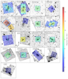 |
Fig. 1. MUSE exposure maps overlaid with HST/F814W images adapted from R21. |
These data have been used for building spectroscopic catalogues providing prior source positions, helping to distinguish overlapping sources detected in the MUSE cubes.
2.3. Identification of LAEs
The construction of MUSE spectroscopic catalogues is documented in R21. To detect line emissions, we made use of MUSE Line Emission Tracker (Muselet), a Python package written by J. Richard1. In turn, this makes use of SExtractor (Bertin & Arnouts 1996) to detect emission line objects on MUSE narrowband continuum subtracted images. To account for low surface brightness sources such as some extended LAEs, a set of given SExtractor detection parameters (DETECT−MINAREA, DETECT−THRESH) have been used to make sure these faint sources are extracted properly. This set of parameters varies among these clusters. Sometimes, a spatial filter is also used by Muselet for smoothing NB images. A spatial filter (5 × 5 tophat with  ) has been used for A2390, A2667, MACS0257, MACS0451, MACS0520, MACS0940, MACS2214, SMACS2031, and SMACS2131. Another (5 × 5 tophat with
  ) has been used for A2744 and A370.
We also made use of the source inspector package, designed by the MUSE collaboration (Bacon et al. 2023), using a combination of both deep HST and MUSE observations to identify sources and their redshifts. Depending on the nature of emission line objects, such as their signal-to-noise ratio (S/N) and the clarity of line absorption and emission features, redshift confidence levels are assigned. A source with zconf = 1 is considered as a tentative case due to either a low S/N or the presence of ambiguous emission lines that do not display a typical Lyman alpha asymmetry profile or various low-S/N absorption properties. A source with zconf = 2 is assigned based on emission lines having a higher S/N compared to the previous case. Such sources may display several absorption lines with low S/N. The confidence level will be upgraded if the source belongs to the multiple imaged systems. The highest level zconf = 3 is for the sources with a high S/N of Lyman-alpha line displaying a typical asymmetry shape and is accompanied by several emission and absorption lines showing the right typical profile. The catalog of sources of the 17 clusters including redshift and spectral line information can be accessed online2 (see R21, for more details). In the present work, there are such 190 unique LAEs categorized as zconf = 1. However, for the purposes of our analysis, we only considered LAEs with secure redshifts (zconf= 2 and 3), excluding all tentative sources with a zconf of 1. The identification of LAEs is described in detail in DLV19, and is also mentioned in Claeyssens et al. (2022).
It is important to note, with respect to sources detected both by HST, called P (prior) sources and by MUSE M sources, that R21 retained the spatial positions of the P sources. We found an average position offset ∼0.2″ between P and M sources. As the LAEs are detected by MUSE, we naturally used the M positions for these sources.
Around 1350 Lyman alpha images with zconf > = 1 have been identified behind the 17 lensing clusters. Many of them are multiple image systems. To avoid counting them more than once, for each multiple image system, we chose a representative image. This also helps to avoid de-lensing them which is computationally expensive. Choosing the representative for each multiple system is manually performed by investigating them one by one. The HST images3 and4 and MUSE white light images are useful for this selection process. If possible, the chosen representative has high enough S/N, reasonable magnification errors and a position that is well isolated, with little to no contamination from nearby bright sources. Finally, 600 LAEs sources were selected at this stage with, in some cases, several different images equally good to represent the parent source. All these sources exhibit zconf = 2 or 3. Their redshift distribution is shown in Fig. 2, together with those from previous work of DLV19 for comparison. A large number of LAEs in the present work have redshifts in the range of 2.9–4.0. There are two bumps in the distribution at redshifts of ∼4 and ∼5, suggesting some overdensities along the line of sight.
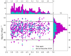 |
Fig. 2. Lyman α luminosity vs. redshift of lensed LAEs in the present work (magenta) and those of DLV19 (cyan). Histograms of redshift (top) and of luminosity (right) are also shown, respectively. |
3. Modeling lensing clusters mass distributions
3.1. Mass distributions by LENSTOOL
There are two approaches that are typically adopted in lens modeling: parametric mass modeling and free-form (non-parametric) methods. For the present work, we use the former to build the total mass distribution of lensing clusters, based on Lenstool (see e.g., Kneib et al. 1996; Jullo et al. 2007; Jullo & Kneib 2009). Following Lenstool, as well as the procedure described in DLV19 and R21, we assume two components contribute to the lensing: 1) the large-scale structure of the cluster 2) the contribution from each massive cluster member. The contribution and implementation of each component is well described in Jullo et al. (2007).
Parameters of individual mass profiles are sampled via a Markov chain Monte Carlo (MCMC) method to compare the match between the observed and predicted multiple images. Details of the lens modeling are described in R21. The lens models and their parameters are listed in Table A.1. Twelve out of the seventeen lens models used in the present work come from the work of R21. Thanks to these models, we can work back and forth between the image and source planes for all LAEs. This allows us to correct for the amplification factor, namely, the lensing magnification, for each source, as well as the source plane projected area allowing us to capture the extended morphology of LAEs.
We note that magnification associated with a given source obtained from Lenstool is the magnification of the source centre, not the entire source. If the LAE in question is a compact one and is relatively far from the lens caustic lines, then it is fair to assign this magnification to that source. Such is the case for 90% sources in the sample. However, for extended sources, in particular those close to the lens caustic lines, magnification strongly varies across the source and using the central point magnification is not justified. In such cases, we must take the flux-weighted magnification by averaging the magnification over the entire source. In this work, we use this weighted magnification for all LAEs. We can do so systematically by using the segmentation map which is created from the NB image by Sextractor and is used as a mask for NB fluxes of the LAEs, to switch back and forth between the image and source planes. Figure 3 displays the difference in magnification between the central and the flux-weighted values for the LAEs in the present sample.
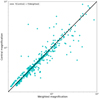 |
Fig. 3. Source central magnification vs. its flux-weighted average one for LAEs in the sample. Extended sources often have averaged magnification values lower than those of their central ones, as expected. The black dashed line denotes a one to one magnification ratio. |
3.2. Flux measurement
We considered two methods to measure fluxes of LAEs. Fluxes were either extracted by fitting the Lyman-alpha (Lyman α) profile as performed by Claeyssens et al. (2022) or by running SExtractor with FLUX−AUTO on the NB images in which the LAEs are detected as performed by DLV19. The first method was employed for LAEs behind 16 lensing clusters except for the A2744, while the second method is applied for the cases in which the first method fails to fit the Lyman alpha profile. Using the first method, we obtained flux measurements for 425 LAEs. However, 47 faint source fluxes could not be measured using this approach. In such cases, we employed the SExtractor package (second method) to extract the fluxes. A large fraction of these failed sources has a low S/N, but they have been upgraded to zconf = 2 because they are members of multiple imaged systems. Furthermore, we used the second method to extract LAE fluxes for sources located behind the lensing cluster A2744. The reason for this is that the source offset positions of the M sources are not available in the new catalogs provided by Claeyssens et al. (2022), whereas the results in DLV19 are in line with the other literature. Overall, we obtained 425 source fluxes using the first method and 175 source fluxes using the second method. We expand briefly on both methods below.
Regarding the first method, Claeyssens et al. (2022) extract LAE fluxes via three main steps: spectral fitting, NB image construction, and repeating spectral extraction. First, a pseudo NB image of each slice (measuring 5″ × 5″) is constructed from the MUSE datacube, using the formulae introduced by Shibuya et al. (2014) to fit the asymmetric spectral profile of LAEs:
![Mathematical equation: $$ \begin{aligned} f(x)=A \ \mathrm{exp}\left[\frac{-(\lambda -\lambda _0)^2}{2(a_{\rm asym}(\lambda -\lambda _0)+d)^2}\right] ,\end{aligned} $$](/articles/aa/full_html/2023/10/aa46716-23/aa46716-23-eq11.gif) (1)
(1)
where A is the flux amplitude, λ0 is the wavelength layer in which source’s emission reaches maximum, aasym accounts for the asymmetry of the Gaussian function, and d is the width of the line. The mean value of d is 7 Å, and the mean value of aasym is 0.20. The value of λ0 is converted directly from source redshift and the flux amplitude A is integrated in the range of [λ0 − 6.25: λ0 + 6.25] Å.
It is worth mentioning that 31 out of the 600 LAE spectra display similar two-peak profiles. We apply the same procedure as described above, dealing with the blue and red peaks separately, taking into account the amplitude difference between the two. The two peaks are then summed to get the final flux. The flux uncertainty is estimated using python package EMCEE (Foreman-Mackey et al. 2013) with 8 walkers and 10 000 iterations.
For the second method, we made use of the SExtractor software (Bertin & Arnouts 1996) running on NB detection images that host LAEs. This is well described in DLV19. For this purpose, a sub-cube with a size of 10″ × 10″× the width of the Lyman-α emission is first extracted from the original cube, then averaged to form the LAE image. Two sub-cubes of the same spatial size, extending 20 Å bluewards and redwards of the Lyman-α line were also created. These were then averaged to form the mean continuum image of each LAE. By subtracting this mean image from the LAE image, pixel by pixel, we can form a new measurement image which is ready for SExtractor. We used SExtractor’s FLUX−AUTO parameter to estimate the LAE fluxes together with their uncertainties. This parameter is developed based on Kron’s first-moment algorithm: when a given source is convolved with a Gaussian seeing, 90% of its flux will be inside the circular aperture of the Kron radius. This holds even for extended sources. The final flux obtained from the measurement image is then multiplied by the width of the Lyman-α emission.
It may happen that some sources are either faint or have a low extended surface brightness. In such cases, SExtractor does not extract these sources properly. A set of farsighted SExtractor parameters (DETECT−THRESH, DETECT−MINAREA) have been proven to be very useful to overcome this problem. SExtractor progressively releases detection conditions using this set of parameters to make sure that faint sources can be extracted.
Figure 4 shows a comparison between the fluxes of LAEs obtained by using the two methods in the present work. In general, the two fluxes agree well with each other within a range of a few orders of magnitudes. The deviation spreads out at the faint fluxes, as expected, but no systematic trend is observed. The source fluxes, obtained from the second method, will be used later to estimate the systematic uncertainties attached to the faint end slope.
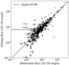 |
Fig. 4. Fluxes of LAEs in the sample, obtained by fitting Lyman-alpha profiles (Claeyssens et al. 2022) vs. those extracted by SExtractor. Solid black line indicates the best linear fit between two the fluxes. |
As mentioned in the previous subsection, to obtain the intrinsic luminosity of a source, its segmentation map is projected into the source plane using Lenstool, then the weighted (averaged) magnification over that source is calculated. The weighted magnifications obtained this way are used throughout this work. The source intrinsic luminosity is computed as:
 (2)
(2)
where FLya is the flux of the LAE obtained as described above, DL is luminosity distance, and μ is weighted average magnification. The luminosity versus redshift and luminosity histogram of our sample together with the ones from DLV19 are shown in Fig. 2.
4. Building the LF
4.1. The Vmax method
In order to deal with the complexity of the lensing datacubes obtained by MUSE, we adopt a non-parametric approach, the 1/Vmax method (Schmidt 1968), allowing us to treat each source individually, to build the LF using detected LAEs behind lensing clusters. The Vmax of a source is the volume of the survey where that individual source could be detected. Inverting this gives the contribution of that source to a number density of galaxies. Determining Vmax is the crucial step in building the LF and this is challenging. We note that noise is an important factor. The Vmax has to take into account noise introduced by the instrument, by sky line variations for different wavelength layers and by local noise variations for different sky directions in the MUSE FOVs. It must take into account the source detectability in all the MUSE lensing datacubes involved in the survey, namely, the whole survey volume. Additionally, it has to be calculated in the source plane to avoid adding the same survey volume for multiple image systems. All of these steps make Vmax determination complex and computationally expensive.
DLV19 developed a package to compute Vmax of lensed LAEs behind lensing clusters observed by MUSE. Details of the algorithm are described in DLV19. Here, we briefly summarize the important points and main steps of the procedure.
Detectability masks are an important concept for computing Vmax. They are built first in the image plane, by comparing a given source brightness distribution pixel by pixel to the RMS maps, channel by channel, in the spectral range of all 18 datacubes. These masks are projected in the source plane using Lenstool, to obtain source plane masks. However, performing this for all sources is extremely computationally expensive. The main important point proposed by DLV19 is to build a set of pre-computed 2D detection masks that cover a wide range of S/Ns for each MUSE datacube. Hence, for a given source, one first computes its S/N in the parent cube, in which the source is detected, then picks up the corresponding 2D mask from the pre-computed list available, which is closest match with the input in terms of S/N. We can do so given that for each lensing datacube root mean square (RMS) maps of different layers display roughly the same type of patterns. One can choose a representative of these RMS maps, namely, their median map, then scale it accordingly by a constant factor to get other RMS maps for different layers. Another important simplification is that for each lensing cluster, we can use a representative brightness profile for all the sources, namely, the median of radial source brightness profiles (see Fig. 5). Using both median radial profile and median RMS map, we can then produce masks at wide range of S/N covering the source sample. This is another simplification to limit the number of masks created in both the image and source planes.
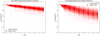 |
Fig. 5. Examples of normalized bright pixels profiles of sources from clusters AS1063 and BULLET. Individual profiles (red) are shown together with their median (black). Each of these median profiles is then used as a representative for all sources in that MUSE datacube. The different seeings between datacubes are taken into account when producing these profiles. The median profile and the RMS map are used to produce a wide range of S/N values for each MUSE datacube. |
The Lenstool package is used to perform the reconstruction from image plane to source plane. To account for variations of projected source plane area as a function of redshift, each 2D mask reconstruction is sampled at four different redshifts, z = 3.5, 4.5, 5.5 and 6.5. One of the four source plane masks is then assigned for a given source, namely, the one that is the closest match to its redshift. Source plane magnification maps are also used to eliminate regions with insufficient amplification implying sources could have not been detected there. The 3D masks for a given source are formed in this way. The final volume is integrated from the unmasked pixels of these 3D source plane masks:
 (3)
(3)
where N is number of unmasked pixels counted on all wavelength layers, ω is the angular size of a pixel, DL is the luminosity distance, and  . The co-volume probed by each cluster of the survey is listed in Table 2.
Total co-volume of 17 clusters (2.9 < z < 6.7).
4.2. Completeness value
Completeness is a correction related to the chance that a given source is detected at its own wavelength affected by random variation of noise on the spatial dimension of the channel, namely, the NB layer where the source’s emission reaches maximum. Together with Vmax, it is a crucial correction before deriving LF points. Depending on source morphology, this completeness is computed individually. Details on how to compute completeness are described in DLV19. We condense the process as follows: 1) A source profile of individual LAE is created from a combination of filtered image, object image, and segmentation image obtained by running SExtractor on the peak NB layer. 2) To compute the completeness for a given source, we have to create the simulations by randomly injecting the source on the masked NB image layer where the emission reaches maximum. We use the real source profile to perform this task. The local noise in the region where the source has been injected is likely to decide whether or not a source is detected. SExtractor scans on the masked NB image, with exactly the same parameters as when that source was originally extracted. We iterate 500 times for each source. The completeness is the detection success rate. 3) The quality of extraction by SExtractor is also taken into account. Following DLV19, sources with flags of type 1 and 2 are trustworthy, but sources with flag 3 are doubtful and will not be used for the LF computation afterwards. From the original sample of 600 LAEs, 588 with flags 1 and 2 are kept at this stage (see more below).
We found that the size of the masked NB images used to re-detect mock sources has an impact on the quality of extractions. When a source has a few neighbors, the local noise is not well represented for that wavelength slice if the size of the image is not large enough. To deal with this, we increased the size from 30″ × 30″ (as in DLV19) to 80″ × 80″. This is more computationally expensive but better accounts for the local noise. The extraction results for the sample are: 555 cases with flag 1; 33 with flag 2; and 12 with flag 3. Additionally, aiming to include as many sources as possible for calculating the contribution to cosmic re-ionization, all sources with completeness values above 1% are retained. Taking this into account, 575 LAEs are used for the next steps.
Figure 6 shows the completeness of each LAE vs. their respective detection flux in the sample. The average completeness value is 0.69 and the median value is 0.90 over the entire sample. The equivalent values from DLV19 are 0.74 and 0.9, respectively. Our average value is a bit smaller than that of the previous work due to numerous faint sources in our sample, which often have low completeness values.
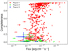 |
Fig. 6. Completeness vs. detection flux of LAEs from the present sample. Different colors indicate the quality of extraction from SExtractor. Only sources in the unmasked regions of the detection layer are considered here. |
For a given source, one may expect that higher its detection flux leads to higher completeness value. However, it is not always the case as shown in Fig. 7. Some sources still have low completeness values, that is, below 0.2, while their detection fluxes are relatively high. It suggests that source morphology also plays an important role in its completeness, as previously mentioned by DLV19.
 |
Fig. 7. Detection flux vs. redshift for all sources in the present sample. The color bar on the top shows completeness value of each source in the sample. The grey points show the evolution of noise level as function of wavelength/redshift for the cluster MACS0257 as an example. |
4.3. Luminosity function determination
We divide the 575 LAEs into four redshift bins in order to study the evolution of the LF with redshift: 2.9 < z < 6.7, 2.9 < z < 4.0, 4.0 < z < 5.0, 5.0 < z < 6.7. The contribution of each individual LAE in each bin is calculated as follows:
 (4)
(4)
where i corresponds to the luminosity bin, Δlog Li is the width of the luminosity bin in log scale, j corresponds to the source in the sample, and Cj and Vmax,j are the completeness value and survey volume of the source in bin i.
We used MCMC to calculate the mean and the statistical uncertainty for each LF point by randomly generating a set of magnification, flux and completeness values for each individual source. 20 000 catalogs were built from the original catalog. For each LAE, the flux and completeness are randomly sorted following Gaussian distributions having means as their measured values and sigmas as their uncertainties. A random magnification value is taken from the magnification distribution P(μ) of each source, accounting for extended source morphology and uncertainties in the lens model. With respect to DLV19, we have introduced an improved procedure to determine the Vmax associated to a random value of the magnification. This allows us to better capture the variations in Vmax taking place for very large values of the magnification. For each iteration, a single value of the LF is obtained for each luminosity bin. The distribution of LF values in each bin, obtained in this way, is used at the end of the process to determine the median of ϕ(Li) in each luminosity bin in linear space, and to compute the asymmetric error bars.
For the estimation of the cosmic variance, we used the cosmic variance calculator presented in Trenti & Stiavelli (2008). A single compact geometry made of the union of the effective (lensing-corrected) areas of the 18 FoVs is assumed following DLV19.
4.4. Schechter function fitting
After obtaining the LF points following the procedure explained above, we fit the results using a Schecter function. The Schechter function, proposed by Schechter (1976), has been extensively used to describe the LF as well as its evolution with redshift. It is often written as:
 (5)
(5)
where: Φ* is a normalization parameter, L* is the luminosity at the point where the power law changes to an exponential law at high luminosity, L is the luminosity, α is the faint end slope, and Φ is the number density in a given of logarithmic luminosity interval.
Regarding the fitting method, we adopted the same procedure as described in DLV19, using a Schechter function with three free parameters to vary (Φ*, L*, α). We first minimized these parameters by using the Levenberg-Marquardt algorithm, in particular, using traditional chi-square minimization procedure, provided by the standard package Lmfit.
5. Faint end of the LF
5.1. Faint-end LF
The faint-end slope of the LF function is still a matter of debate and more observations are strongly needed. Strong gravitational lensing by clusters of galaxies is of great help to probe the faint galaxy luminosity regime and hence to constrain the shape of LF in that region. The price to pay is that the cosmic volume of the survey is significantly reduced: the higher the lensing magnification factors, the lower the volume probed. Our sample efficiently probes down to 1040 erg s−1, the same faint luminosity regime as studied by DLV19 but with improved statistics and a better coverage at the faint end of the luminosity distribution (see Fig. 2) and 34 000 Mpc3 larger co-volume explored accounting for the magnification in the range of redshifts 2.9 < z < 6.7. On the contrary, the MUSE Wide and other deep blank fields surveys cover well the bright luminosity part (see Drake et al. 2017; Herenz et al. 2019). These studies are efficient to probe the LF around the log L* regime, while the sample in this work is optimized to probe the faint-end part.
For a first attempt, we try to fit the LF with a linear fit to find the slope at the faint end. We only used our LF points, computed from the 575 LAEs. We considered four different redshift bins, 2.9 < z < 4.0 (z35), 4.0 < z < 5.0 (z45), 5.0 < z < 6.7 (z60), 2.9 < z < 6.7 (zall) to make these fits. The results are shown in Fig. 9. The respective slopes are  ,
,  ,
,  and
and  . In spite of our bigger sample, four times more sources than in DLV19, spanning over four orders of magnitudes in galaxy luminosity, we essentially obtain the same results: no evolution of the faint end slope as a function of redshift is observed. The current sample suggests that (at face value) the faint-end slope in each redshift range is steeper than for DLV19, for the same redshift interval. However, as seen in Fig. 9, a turnover seems to appear at luminosities fainter than 1041 erg s−1, for the two highest redshift bins. This trend is discussed below.
5.2. Computing LF parameters
This section presents the fit of our LF points with the Schechter function. As the luminosity range of our sample reaches its maximum 1043 erg s−1, which is close to values of log L* (Herenz et al. 2019, DLV19), to completely describe the Schechter function, we need to include other data covering the bright end of the LF. The data included are taken from the works of: Dawson et al. (2007), Blanc et al. (2011), Cassata et al. (2011), Zheng et al. (2013), Sobral et al. (2018), Drake et al. (2017) and Herenz et al. (2019), which have been selected to properly cover the redshift and bright part of luminosity ranges. These data from the literature are averaged with the same luminosity bin size of 0.25 (in log10(L) [erg s−1]), except for the last faintest bin which has a width of 1.25 for redshift bin zall, while in the other bins the width is 0.5. This is meant to avoid an increased weight of this bright sample from the literature on the global fit.
The fitting process is performed as described in Sect. 4.4. The results are shown in Fig. 10, with the best fit curves shown as solid lines together with the 68% and 95% confidence area based on the data as indicated in the respective labels. We also check that the shape of the LF for each redshift interval is essentially the same when changing the number of luminosity bins, similarly to DLV19 (Fig. 11).
The best fit parameters are listed in Table 3. The best fit value of log L* is in good agreement with DLV19, and a few percents higher than the value obtained from Herenz et al. (2019), 42.20 . Strong degeneracy between these parameters (Φ*, L*, α) is observed, as shown in Fig. 12, and already well documented in Herenz et al. (2019). Also, log L* seems to be well measured from the current work for different redshift intervals. There is a tendency of L* to increase with redshift but this is well within the uncertainties. As both log L* and the steep faint-end slope increase with redshift, it is likely related to the degeneracy mentioned earlier. Then, Φ* is just a normalization factor giving the number density of objects per given volume. Our best fit result gives Φ* [10−4 Mpc−3] =
  which is consistent with DLV19 and Sobral et al. (2018), but smaller than that of Herenz et al. (2019). The Φ* value strongly depends on the literature data points used for the fitting procedure. Luminosity bins and LF points for each redshift interval are given in Table 4.
Best-fit parameter values for the Schechter function.
As our sample probes the faint luminosity regime, the slope at the faint-end of LF, α, in principle, is well constrained. We measure steep slopes of α varying from −2.0 ± 0.07 for the redshift interval 2.9 < z < 4.0 to −2.28 ± 0.12 for redshift interval 5.0 < z < 6.7. These results are consistent with the slope measured by Herenz et al. (2019) for the global redshift bin, and Drake et al. (2017) in same redshift bins. The faintest luminosity points in all redshift intervals, having log(L) [erg s−1] < 40, are not included in the Schechter’s fitting. As sources in this faintest bin are often highly magnified by lensing effects, namely, sources close to the lens caustic lines, this seems to suggest either that lensing systematic uncertainties or that completeness corrections for those sources must be treated with great care. Another possibility is that the faint end of the LF may depart from the traditional Schechter function. More data in this luminosity regime is required to verify this. The enhancement at log(L) around 42 shown in zall is because the number of sources suddenly increases in that luminosity bin. This is also shown in Fig. 8, where a spike appears at the luminosity bin log(L) [erg s−1] ∼ 42 after correcting for completeness. This may relate to the over-density of background sources at z ∼ 4 as mention in DLV19. This may also suggest the uncertainty from the cosmic variance is probably larger than expectations. The co-volume probed by our survey is ∼50 000 Mpc3. It seems that the data points from Drake et al. (2017) and Cassata et al. (2011) within the log(L) range of 41.5–43.0 might influence the fitting results of the faint end slope z35 and z60. However, we checked and found that including or excluding these data points does not substantially alter our results. The faint end slopes at these specific redshift ranges show only minor variations less than a few percent.
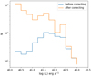 |
Fig. 8. Source distribution in each luminosity bin (the faintest on the left, the brightest on the right) before and after correcting for the completeness. A larger correction, a factor up to a few tens, has been made at the faint luminosity regime, as expected. |
5.3. Error budget
The uncertainties on LF points are well documented in DLV19. There are three kinds of uncertainties attached to the LF points which are addressed. The statistical uncertainty is derived from the MCMC process. A set of flux, magnification, and completeness associated with each LAE is randomly drawn 20 000 times. The results are then used to estimate the mean and statistical uncertainties attached to each LF point. The second source of uncertainty relates to field-to-field variance for different lensing FoVs observed by MUSE. We use the cosmic variance calculator proposed by Trenti & Stiavelli (2008) to estimate this uncertainty, which is typically about 20%–30% at most. The third one, the Poissonian uncertainty, relates to the number of sources for a given luminosity bin, which is relatively easy to handle. For the bright-end luminosity, log(L) [erg s−1] > 42, the Poissonian uncertainty dominates. Its contribution decreases and becomes equivalent to that of cosmic variance in the luminosity range 41 < log(L) [erg s−1] < 42. The statistical uncertainty is dominant in the faint-end regime.
One would expect systematic uncertainty coming from lensing models to be another important contribution to the total error budget. Different lensing models may give magnification factors that differ by a significant factor for a given source, increasing the uncertainty on the luminosity obtained. This systematic uncertainty is well documented in Bouwens et al. (2017), Atek et al. (2018), Priewe et al. (2017), Meneghetti et al. (2017). It might play important role in particular to the faint end luminosity regime. As discussed in DLV19 its contribution is ∼15% at log(L) of 40.5 erg s−1 for the case of the lensing field A2744.
6. Discussion
6.1. Uncertainties associated to the computation of the LF in strong lensing fields
Thanks to the magnification by lensing clusters, we can reach a fainter galaxy population compared to that of Drake et al. (2017) and Herenz et al. (2019) by one order of magnitude, allowing us to constrain the faint-end slope of the LF. Although the number of sources in the previous sample by DLV19 is four times smaller, it still covered by the same luminosity range as in the present project. Three lensing clusters, which were previously studied in DLV19, have been re-reduced to achieve better quality in terms of S/N and source positions.
In this work, when sources are both detected by HST and MUSE, we used the Muselet positions (M pos.) instead of prior ones from HST observations (P pos.). Choosing these positions has some impact on the LF shape at the faint end. An average spatial offset of ∼0.2 arcsec between the M and P positions has been found in Claeyssens et al. (2022). MUSE observations are sensitive to detect line emissions such as Lyman-alpha while HST ones are sensitive to continuum emission. It may happen that the LAEs are extended and associated with diffuse gas, hence the offset between the two observations.
Moreover, the faint luminosity regime often contains highly magnified sources. These sources are close to the lens caustic lines in the source plane, hence, their positions have to be assessed with great care. The weighted magnifications for these extended sources strongly depend on their positions with respect to the caustic lines. In addition, the magnification uncertainties attached to these sources are also large and this may cause the source contribution to spread to several luminosity bins during the MCMC process to estimate LF point uncertainties. On the contrary, sources in the bright luminosity bins usually have small magnifications and do not suffer from this effect. In principle, the procedure adopted here to compute the LF points captures all these effects.
An important point to note is that DLV19 used a threshold of 10% completeness to reject sources having completeness values below this cut. A small completeness value implies a large correction on the number of detected sources (see Fig. 8). Varying the completeness threshold cut significantly changes the shape of the LF at the faint end as one may loose some fraction of these sources. In the present work, we try to include as many sources as possible from the sample, only rejecting obvious cases which have a poor extraction quality, namely, flag type 3 as identified from SExtractor. In practice, we used a cut in completeness of 1%, meaning that a final sample of 575 LAEs is used for the LF computation. In the global redshift bin, zall, and z35 (see Fig. 10), the number density of sources suddenly increases at log(L) [erg s−1] ∼ 42; this is also caused by the low completeness values for some sources in that luminosity bin. It is worth noting that usual computations of the LF in lensing fields do not reject any source based on its completeness value (see e.g., Atek et al. 2018). By implementing a 10% completeness, we further removed 62 additional sources from our sample, with 51 of them belonging to the six faintest luminosity bins. As a result, the density of source significantly reduces by a factor of 5 on average. The faint end slope decreases from its original value of −2.06 to a flatter value of −1.46 for the global redshift range Table 5. This reveals insights into the uncertainties associated with the faint end slope, which we discuss in detail in the subsequent subsection.
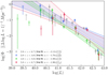 |
Fig. 9. Faint-end slope of LF: Line (power law) fitting for four different redshift ranges: 2.9 < z < 4.0 (blue), 4.0 < z < 5.0 (green), 5.0 < z < 6.7 (red), and 2.9 < z < 6.7 (black). These fits only use our LF points constructed from the current sample. Open symbols at the faintest luminosity bins are not included in the fitting process. |
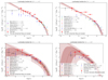 |
Fig. 10. LF points and their fits for different redshift intervals including previous literature data points. The red squares are the points from the present work. The literature points at the bright end of the LF: Ouchi et al. (2010), Sobral et al. (2018), Zheng et al. (2013), Herenz et al. (2019), and Drake et al. (2017) have been used for the fitting. The blue points DLV19 are shown for comparison purpose only. The best fits (Schechter function) are shown as a solid line and the 68% and 95% confidence areas as dark-red colored regions, respectively. The dashed lines shown in lower panels are modified Schechter functions to account for a possible turnover at faint luminosity bins (see details in the text). |
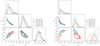 |
Fig. 11. Correlations between three Schechter’s best-fit parameters for different luminosity bins. The tuples denote the lower and upper limit of the luminosity range with respect to the number of the bin. Contours are 68% confidence levels obtained from the Schechter’s fitting. Results are shown for 2.9 < z < 6.7 (left) and 4.0 < z < 5.0 (right). |
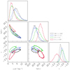 |
Fig. 12. Correlations between the three parameters, L*, Φ* and α of the Schechter function for four different redshift bins as indicated in the inserted. Contours show 68% confidence levels obtained from fitting procedures. |
Results of the faint end slope α from different tests.
6.2. Comparison with previous results
In the bright luminosity regime (log(L) [erg s−1] > 40.5), the data from the literature mainly come from blank field observations. They are numerous and helpful to constrain the LF at the bright end. Indeed, we include some of them from blank fields for the fitting procedure to constraint the bright-end part of the LF. Blanc et al. (2011) used 89 LAEs with a redshift range 1.9 < z< 3.8 obtained from Hobby Eberly Telescope Dark Energy Experiment Pilot Survey (HETDEX) to study the LF using the same Vmax method. Drake et al. (2017) used 604 LAEs in the redshift range 2.91 < z< 6.64 obtained from VLT/MUSE. Cassata et al. (2011) used 217 LAEs in the redshift range 2 < z< 6.62 obtained from Vimos-VLT Deep Survey. Sobral et al. (2018) studied ∼4000 LAEs from z ∼ 2 to 6 covering a luminosity range of 42.4 < log (L) [erg s−1] < 43.0 obtained from the Subaru and the Isaac Newton Telescope in the ∼2deg2 COSMOS field. Our LF points in the bright part (log(L) [erg s−1] > 42) are consistent with these results from the literature (Fig. 10).
It is worth mentioning the work of Herenz et al. (2019). They used data including 237 LAEs from the MUSE Wide survey to construct the LF in the same redshift ranges as this work. They found the faint-end slope value at redshift 2.9 < z < 6.7 to be  , log Φ* [Mpc−3]= − 2.71 and log L*[erg s−1] = 42.20
 . Comparing to our results, the two slopes at the faint end are consistent while their best fit of log L* is a bit smaller. The explanation may relate to the degeneracy between the three best fit parameters. We note that Herenz et al. (2019) constructed LAEs LF in the luminosity range 42.2 < log(L) [erg s−1] < 43.5.
It is necessary to compare our results with those obtained by DLV19, which also probe the faint luminosity regime. The characteristic log L* is well measured both in different redshift intervals and in different cluster samples. The best-fit values agree well with each other, within their 1-σ uncertainties. However, the present slope values are steeper by 20% than those from the previous work for the same redshift intervals. The difference between the two may be due to various factors. Firstly, the number of sources in the two samples differ: we have four times more sources in the present sample, giving us better statistics. Our sample has a significant number of sources in the faint luminosity region and more than ten sources in the faintest bin. Secondly, the threshold cuts in completeness are different. DLV19 rejected faint sources with completeness values below 10%, while we have included as many sources as possible, for consistency with other LF determinations in lensing fields, rejecting only those with completeness values below 1%. Thirdly, as explained above, our MCMC procedure to compute the LF points better captures the relationship between magnification and Vmax with respect to DLV19. Finally, the number of LF literature data points helping to constraint the bright-end part is different between the two works. The results from Herenz et al. (2019) using MUSE-Wide survey to investigate Lyman α LF in the same redshift bin are included and combined with others as a constraint association; the results from Drake et al. (2017) are used for fitting at redshift bin 2.9 < z < 4.0 and for displaying only at others bins. This affects the normalization parameter as well as the faint-end slope, since the two are correlated. We also performed the full analysis with the new improved procedure on the sub-sample of four clusters in DLV19, with the same choices regarding the completeness, and found fully consistent results with DLV19.
One of the important points derived from Fig. 10 is that faint-end slope values of α become steeper at higher redshifts. This seems to suggest the evolution of the faint-end slope as a function of redshift. There is a very good agreement between the slopes obtained from Schechter function fitting and those obtained from line-fitting in Sect. 5.1. However, we do not see the same trend of the slope evolution from line-fitting, which only used our LF points, due to the larger uncertainties associated with them. Moreover, we observe a turnover at luminosities fainter than 1041 erg s−1, for the two highest redshift bins. At these luminosities, the LF points are not well described by the Schechter function. A flattening and turnover are observed towards the faint end for the highest redshift bins that still needs further investigation. This turnover is similar to the one observed at MUV = −15 for the UV LF at z ≥ 6 in lensing clusters, with the same conclusions regarding the reliability of the current results when we compare, for instance, the work of Atek et al. (2018) to Bouwens et al. (2022; see discussion below).
To account for a possible turnover in the two highest redshift ranges 4.0 < z < 5.0 and 5.0 < z < 6.7, two more parameters have been introduced to modify the Schechter function, which is then expressed as:
 (6)
(6)
where: Φ(L) is the traditional Schechter function together with its three (Φ*, L*, α) parameters, being fixed at their best-fit values, as shown in Table 3. Two new parameters are introduced: LT is the luminosity at the turnover point and m is a power index, which is about unity. Our data suggest that log(LT) are ∼40 and ∼40.7 erg s−1 for redshift bins 4.0 < z < 5 and 5.0 < z < 6.7, respectively. The values of m are essentially equal to 1 for these two redshift ranges, as expected. Results are shown in Fig. 10 (lower panels).
Regarding the prevalence of a turnover in the LF towards the faint end, it is worth mentioning that Bouwens et al. (2022) have recently ruled out this trend in the UV LF down to MUV = −14 mag at z ∼ 6. In addition, Dawoodbhoy et al. (2023), using the CODA simulation, reported no sign of the turnover down to MUV = −12 mag at the same redshifts. The large uncertainty in the faint regime of LAE luminosity prevents us to make much sense of this result. Additional data in this faint region are necessary to improve the statistical significance of the present sample in order to confirm or reject this turnover trend.
6.3. Comparison with theoretical predictions
We compared our results on the Lyman-alpha LF with two theoretical models whose predictions at z ∼ 6 can be compared directly with our findings in the highest redshift range of 5.0 < z < 6.7, namely, the predictions of Garel et al. (2021) and by Salvador-Solé et al. (2022). The first one (Garel et al. 2021) predicts the Lyman-alpha LF at the epoch of reionization by computing the radiative transfer of Lyman-alpha from ISM to IGM scales, using the SPHINX radiation-hydrodynamics cosmological simulation. Their results, obtained by computing the intrinsic LF function, and the attenuation by dust and then by IGM, are shown in Fig. 13. The second one (Salvador-Solé et al. 2022) uses the Analytic Model of Igm and GAlaxy evolution (AMIGA), a model of galaxy formation and evolution including their feedback on the IGM, to constrain the reionization history of the universe. It provides predictions for two possible scenarios: single and double reionization episodes. The former has hydrogen ionization episode at z ∼ 6, and the latter has two reionization episodes at z ∼ 6 and ∼10, separated by a short recombination period (see Salvador-Solé et al. 2022, for additional details). Their results for the two scenarios are also shown in Fig. 13. In the range of 40 < log(L)[erg s−1] < 42, the prediction of the AMIGA double ionization scenario is in good agreement with that of Garel et al. (2021) after IGM correction. Our LF points towards the faint end correctly span the region covered by these models. In general, our LF points are in good agreement with the predictions by both models without any renormalization, as shown in Fig. 13. At the faintest luminosity regime, log(L) < 41, our LF point starts to depart from the theoretical increasing trend by Garel et al. (2021), and is somewhat closer to the single ionization scenario predicted by Salvador-Solé et al. (2022). However, the uncertainties in this regime are very large, preventing us to distinguish between the different theoretical predictions. More data covering this faint regime are badly needed.
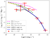 |
Fig. 13. Comparison with model predictions. Red crosses show our reconstructed LF points in the redshift range of 5.0 < z < 6.7. Two additional crosses in the bright end, having log(L)[erg s−1] > 43, are taken from the literature, obtained the same way as described in Sect. 5.2. Black and blue solid lines show predictions from the AMIGA models with single- and double-ionization scenarios, respectively. Predicted LFs from the SPHINX simulation (Garel et al. 2021) are shown as dashed lines: intrinsic LF (magenta), attenuation by dust (green), and by IGM (orange). |
6.4. Effect of source selection
There are several factors that play important roles in determining the faint end slope. One of them is the source selection process. In the 17 lensing clusters, 190 LAEs (unique system) have been classified as zconf = 1, and as a consequence, they are not retained for the LF computation process. However, as they are often faint, they may contribute significantly to our faint LF points. To evaluate the impact of zconf = 1 sources on the final LF points, we have incorporated them into our LAE sample. We assume that zconf = 1 sources have the same quality of completeness and Vmax as the zconf = 2, 3 sources; namely, for a given luminosity bin, zconf = 1 completeness and Vmax values are assigned as the mean values for the zconf = 2, 3. Similarly, the uncertainty values for completeness and Vmax of the zconf = 1 sources are set equal to the corresponding uncertainty values of the zconf = 2, 3 sources in that bin. Including half and all of the zconf = 1 sources results in a 5% and 10% steeper faint end slope, respectively.
To estimate the systematic uncertainties attached to the faint end slope, we performed various tests to calculate the LF points and measured the slope. We employed different completeness threshold cuts (1% and 10%), utilizing different fitting function forms (Schechter and linear functions) and considering two scenarios: including half or all of the zconf = 1 sources. We also used source fluxes obtained from the pipeline only (method 2). Our findings are summarized in Table 5. We retained a faint-end slope of the 1% completeness cut results and increased the uncertainties. The final slope are −2.00 ± 0.50, −1.97 ± 0.50, −2.28 ± 0.50, −2.06 ± 0.60 for z35, z45, z60, zall, respectively. Figure 14 illustrates the faint end slope at different redshift ranges. The slope shows a slight increase with redshift, although the uncertainties remain large. Our slopes at various redshift ranges are in good agreement with the findings of other studies, typically within a 1-σ deviation.
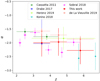 |
Fig. 14. Comparison of slope evolution with redshift from this work (red crosses) to the literature which appears in the Fig. 10. The horizontal error bars are the redshift range of the surveys. |
6.5. Implications for the reionization
One of the most important tools to understand the formation and evolution of galaxies is the cosmic SFRD, providing information on the onset of star formation in the early Universe and its evolution over cosmic time (Madau et al. 1996; Bouwens et al. 2007, 2008). In this section, we present the contribution of LAE population to the cosmic re-ionization by computing the SFRD by integrating the best-fit parameters obtained from the previous section. In addition to the luminosity range of the integral (Eq. (7)), log(L) = (39.5, 44.0) as probed by the present sample, we also chose another lower limit luminosity of 0.03L* ∼ 1041 erg s−1 to facilitate the comparison with previous works. The integrated SFRD is proportional to the luminosity density and can be estimated following the calibration of Kennicutt (1998), assuming an intrinsic factor of 8.7 between the intrinsic Lyα and Hα fluxes, and case B for the recombination (Osterbrock 1989). In that case, all newly formed Lyα photons would be re-absorbed by the neutral hydrogen atoms of the HII region. In the optically thick case, the SFRD is expressed as:
![Mathematical equation: $$ \begin{aligned} \mathrm{SFRD}_{\rm Lya}[{M}_{\odot } \,\mathrm{yr}^{-1}\,\mathrm{Mpc}^{-3}] =\rho _{\rm Lya}/1.05 \times 10^{42} ,\end{aligned} $$](/articles/aa/full_html/2023/10/aa46716-23/aa46716-23-eq71.gif) (7)
(7)
where ρLya is the Lyα luminosity density in units of erg s−1 Mpc−3.
The results are shown in Fig. 15 together with the other literature data from different sources and surveys. The yellow regions show the SFRD needed to fully ionize the entire Universe, taken from the work of Bouwens et al. (2015b) at the level of 1-σ and 2-σ. A clumping factor of 3 is applied to calculate cosmic emissivity, log(ξionfescp) = 24.50, where fescp is escape fraction of ionizing UV photons, ξion is the production efficiency of Lyman-continuum photons per unit UV luminosity. The conversion to SFRD is then calculated as, SFRDLya[M⊙ yr−1 Mpc−3] = ρUV/(8.0 × 1027).
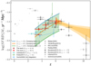 |
Fig. 15. Evolution of the star formation rate density with redshift using different integration limits for the LF. Brown (red) crosses show results of integrating the best-fit Schechter (modified Schechter) functions log(L) from 41 (39.5) to 44 erg s−1. Solid blue, orange, and green curves indicate the critical SFRDs obtained by assuming a clumping factor of 3 and fescp = 3%, 8%, and 25%, respectively. The solid green curve, having fescp = 8%, indicates the best likely match with our SFRD points in the luminosity range of 41 < log(L) < 44 (see details in the text). |
Figure 15 shows the evolution of the SFRD with redshift. As the LF decreases steeply toward the bright end, the upper limit of the integration (Eq. (7)) does not affect to the final result. However, the steep slope at the faint-end plays an important role. If we take the integral over the full range probed by the present sample, the contribution of LAEs to the cosmic re-ionization at redshift z ∼ 3.5 and z ∼ 4.5 would be ∼80%, compared to that of Bouwens et al. (2015b) using MUV = −17 mag as observational limit. At higher redshifts z ∼ 6 the contribution is much higher, 10% larger than Drake et al. (2017), 4 times larger than Cassata et al. (2011), 12 times larger than Ouchi et al. (2008), and much higher than Bouwens et al. (2015a). If we take the lower limit of the integral (Eq. (7)) at 0.03L*, results are shown as reddish-brown crosses, which are more consistent with others mentioned above. Then, the contribution of LAEs population at redshift z ∼ 3.5 is 10%, 30% at redshift z ∼ 4.5, and reaches up 100% at higher redshifts. Figure 15 also shows SFRD reported by Sobral et al. (2018). The difference between our results on the evolution of the SFRD and those obtained by Sobral et al. (2018) can be explained by comparing the detailed shape of the LF and the luminosity range covered by the two studies. Indeed, the shape of the bright end does not affect the SFRD, and our sample better captures the steepening of the LF towards the faint end, which is responsible for the increase of the SFRD with redshift in our case. When using the modified Schechter functions instead of the traditional one to compute the SFRD over the full probed luminosity range, 39.5 < log(L) < 44, in order to better describe the flattening/turnover observed towards the faint end, the contribution is 25%, 50%, and 100%, respectively.
Assessing the ability of a population of sources to reionize the Universe is usually done by comparing its ionizing power to the critical value needed to maintain reionization at a given redshift. This value for the critical photon emission rate per unit cosmological comoving volume was introduced by Madau et al. (1999) as follows:
 (8)
(8)
where C30 is the clumping factor  , normalized to CHII = 30, and nHII is the mean comoving hydrogen density in the Universe. Assuming C30 = 1 and
  , the critical SFRD will be written as:
 (9)
(9)
The clumping factor, C30, can be considered as a correction accounting for inhomogeneities in the IGM, and it is supposed to vary as a function of redshift. For example, as reported by Shull et al. (2012), CHII = 2.9 × ((1 + z)/6)−1.1 (i.e., a value ∼3 at z ∼ 5), hence, the critical SFRD obtained from the equation above needs a correction factor of  . Here, we adopt the average value of CHII = 3, to facilitate the comparison with previous works (Pawlik et al. 2009; Robertson et al. 2013, 2015; Bouwens et al. 2015b; Gorce et al. 2018).
The dependence of Lyα escape fraction on redshift is an important quantity as it helps to constrain the reionization history of the Universe. The Lyα escape fraction  and fescp are expected to be correlated (see e.g., Dijkstra et al. 2016; Izotov et al. 2020), Hayes et al. (2011) reported an evolution as a function of redshift as follows
  ∝(1 + z)ξ, with
  over the redshift range 0.3 < z < 6, reaching a maximum of unity at z = 11.1. The increase in
  with redshift follows the evolution of the dust content in galaxies up to z ∼ 6, and then drops above z ∼ 6.5. Using this prescription in the range covered by our study and a reasonable conversion for fescp, following Dijkstra et al. (2016), the order of magnitude expected for fescp is ∼5% at z ∼ 3 and up to some 25% at z ∼ 6. Figure 15 displays the critical SFRDs obtained from these two extremes of fescp as a shaded area, using the same clumping factor of 3 as described above. As seen in the figure, the SFRD points obtained from our Lyα LF with the integration limits 41 < log(L) < 44 are fully consistent with the critical ones for the average value of fescp ∼ 8% and CHII = 3, in the redshift interval of 3 < z < 6.7. In other words, the contribution of LAEs to the ionizing flux in this redshift interval seems to be sufficient to keep the hydrogen ionized. The contribution of LAEs at z ∼ 6 is comparable to the one provided by LBGs.
This result taken at face values suggests that the contribution of the population of LAEs to cosmic re-ionization could be much higher than previously expected. There are, however, a few caveats to mention. Firstly, the vast majority of previous surveys in blank fields have been focused on the most luminous galaxies in their restframe UV that are well suited for a successful spectroscopic follow up. By construction, these samples can not probe to the faint luminosity regime, down to 1039 erg s−1, as in the present work. In addition, IFU observations identify LAEs without any pre-selection. Secondly, the contribution to the SFRD is directly related to the steep slope value being obtained, which is directly proportion to Lyα luminosity density. A 20% steeper slope dramatically changes the LAEs contribution to the cosmic re-ionization as illustrated here. Thirdly, the lower limit of the integration also has an impact on the final contribution. Moreover, there are still large uncertainties in the Lyαfescp and its evolution with redshift making difficult the comparison between different works using different prescriptions.
7. Conclusions
We present a study of the galaxy Lyα LF using a large sample of 17 lensing clusters observed by MUSE. We blindly selected 600 lensed LAEs behind these clusters in the redshift range of 2.9 < z < 6.7. The sample covers four orders of magnitude in galaxy luminosity (39.0 < log(L) < 44.0) and efficiently probes the faint luminosity regime, down to 1040 erg s−1. This sample sets a strong constraint on the LF at the faint end as well as the evolution of the slope as a function of redshift.
To deal with the combination of lensing fields and spectroscopic datacubes obtained from MUSE, we adopted the same Vmax method and the same procedure as described in DLV19 to compute the LF points. Several improvements have been introduced and applied to the original pipeline, allowing us to better account for lensing magnification. The main results and conclusions are listed as follows:
– Regarding the method and the pipeline, several effects have been studied in details, with the corresponding improvement on the final results with respect to DLV19. The new pipeline better accounts for the magnification errors when computing Vmax. A careful analysis was performed on the effects of source centering and completeness corrections.
– We studied the LF in four redshift bins, 2.9 < z < 4.0, 4.0 < z < 5.0, 5.0 < z < 6.7, and 2.9 < z < 6.7. The total co-moving volume of our survey is ∼50 000 Mpc3. With respect to the previous work by DLV19, A2744 is still the dominant cluster, with a contribution to the total volume three times above the average.
– The three best-fit parameters of the Schechter function in the redshift range 2.9 < z < 6.7, obtained from our sample, are:  , Φ*[10−4 Mpc−3] =
  , log(L*)[erg s−1] =
  .
.
– The LF values in the bright-end regime (log L > 42) are consistent with previous works, in particular the MUSE-Wide observations, as well as with other surveys in the literature using different techniques.
– In the faint luminosity regime, the contribution of highly magnified sources to the LF points in the faint luminosity bins is significant, as expected. The density of sources is well described by a steep slope, α ∼ −2. The two slopes obtained from line-fitting and from the Schechter function are consistent within their uncertainties. The present Schechter slope is consistent with those from Drake et al. (2017) for each redshift interval, following Herenz et al. (2019) for the global redshift range, and is 20% steeper than the slope of DLV19. When taking into account different flux measurements, different completeness threshold cut (1% and 10%), and source selection effects, we obtained faint end slopes of −2.00 ± 0.50, −1.97 ± 0.50, −2.28 ± 0.50, and −2.06 ± 0.60 for z35, z45, z60, and zall, respectively. These results are in line with other studies, typically within a 1-σ deviation.
– The steepening of the faint end slope with redshift, suggested by the earlier work of DLV19 is confirmed here, but the uncertainties remain large. A turnover seems to appear at luminosities fainter than ∼1041 erg s−1, for the two highest redshift bins.
– The SFRD depends strongly on the interval of luminosity over which the density is integrated. The steeper slope at the faint end causes the SFRD to dramatically increase between z ∼ 3 and 6, implying that LAEs play a major role in the process of cosmic reionization.
– The contribution of LAEs to the ionizing flux in the redshift interval studied here seems to be sufficient to keep the hydrogen ionized. The contribution of LAEs at z ∼ 6 is comparable to the one provided by LBGs.
Acknowledgments
We are grateful to the referee for a very careful reading of the manuscript and pertinent comments that helped greatly with improving the substance of the present article. This work is done based on observations made with ESO Telescopes at the La Silla Paranal Observatory under programme IDs 060.A-9345, 094.A-0115, 095.A-0181, 096.A-0710, 097.A0269, 100.A-0249, and 294.A-5032. Also based on observations obtained with the NASA/ESA Hubble Space Telescope, retrieved from the Mikulski Archive for Space Telescopes (MAST) at the Space Telescope Science Institute (STScI). STScI is operated by the Association of Universities for Research in Astronomy, Inc. under NASA contract NAS 5-26555. This research made use of Astropy, a community- developed core Python package for Astronomy (Astropy Collaboration 2013). All plots in this paper were created using Matplotlib (Hunter 2007). Financial support from the World Laboratory, the Odon Vallet Foundation and VNSC is gratefully acknowledged. Tran Thi Thai was funded by Vingroup JSC and supported by the Master, PhD Scholarship Programme of Vingroup Innovation Foundation (VINIF), Institute of Big Data, code VINIF.2022.TS.107. This work received support from the French government under the France 2030 investment plan, as part of the Excellence Initiative of Aix-Marseille University – A*MIDEX (AMX-19-IET-008 – IPhU).
References
- Astropy Collaboration (Robitaille, T. P., et al.) 2013, A&A, 558, A33 [NASA ADS] [CrossRef] [EDP Sciences] [Google Scholar]
- Atek, H., Richard, J., Kneib, J.-P., & Schaerer, D. 2018, MNRAS, 479, 5184 [Google Scholar]
- Bacon, R., Accardo, M., Adjali, L., et al. 2010, in Ground-based and Airborne Instrumentation for Astronomy III, eds. I. S. McLean, S. K. Ramsay, & H. Takami, SPIE Conf. Ser., 7735, 773508 [Google Scholar]
- Bacon, R., Brinchmann, J., Conseil, S., et al. 2023, A&A, 670, A4 [NASA ADS] [CrossRef] [EDP Sciences] [Google Scholar]
- Beauchesne, B., Clément, B., Hibon, P., et al. 2023, MNRAS, submitted [arXiv:2301.10907] [Google Scholar]
- Bertin, E., & Arnouts, S. 1996, A&AS, 117, 393 [NASA ADS] [CrossRef] [EDP Sciences] [Google Scholar]
- Blanc, G. A., Adams, J. J., Gebhardt, K., et al. 2011, ApJ, 736, 31 [CrossRef] [Google Scholar]
- Bouwens, R. J., Illingworth, G., Ellis, R. S., Oesch, P., & Stefanon, M. 2022, ApJ, 940, 55 [NASA ADS] [CrossRef] [Google Scholar]
- Bouwens, R. J., Illingworth, G. D., Franx, M., & Ford, H. 2007, ApJ, 670, 928 [Google Scholar]
- Bouwens, R. J., Illingworth, G. D., Franx, M., & Ford, H. 2008, ApJ, 686, 230 [NASA ADS] [CrossRef] [Google Scholar]
- Bouwens, R. J., Illingworth, G. D., Oesch, P. A., et al. 2015a, ApJ, 811, 140 [NASA ADS] [CrossRef] [Google Scholar]
- Bouwens, R. J., Illingworth, G. D., Oesch, P. A., et al. 2015b, ApJ, 803, 34 [Google Scholar]
- Bouwens, R. J., Illingworth, G. D., Oesch, P. A., et al. 2017, ApJ, 843, 41 [Google Scholar]
- Cassata, P., Le Fèvre, O., Garilli, B., et al. 2011, A&A, 525, A143 [NASA ADS] [CrossRef] [EDP Sciences] [Google Scholar]
- Claeyssens, A., Richard, J., Blaizot, J., et al. 2022, A&A, 666, A78 [NASA ADS] [CrossRef] [EDP Sciences] [Google Scholar]
- Covone, G., Kneib, J. P., Soucail, G., et al. 2006, A&A, 456, 409 [NASA ADS] [CrossRef] [EDP Sciences] [Google Scholar]
- Dawoodbhoy, T., Shapiro, P. R., Ocvirk, P., et al. 2023, MNRAS, 524, 6231 [Google Scholar]
- Dawson, S., Rhoads, J. E., Malhotra, S., et al. 2007, ApJ, 671, 1227 [NASA ADS] [CrossRef] [Google Scholar]
- Deharveng, J.-M., Small, T., Barlow, T. A., et al. 2008, ApJ, 680, 1072 [NASA ADS] [CrossRef] [Google Scholar]
- de la Vieuville, G., Bina, D., Pello, R., et al. 2019, A&A, 628, A3 [NASA ADS] [CrossRef] [EDP Sciences] [Google Scholar]
- Dijkstra, M., Gronke, M., & Venkatesan, A. 2016, ApJ, 828, 71 [Google Scholar]
- Drake, A. B., Garel, T., Wisotzki, L., et al. 2017, A&A, 608, A6 [NASA ADS] [CrossRef] [EDP Sciences] [Google Scholar]
- Fan, X., Strauss, M. A., Becker, R. H., et al. 2006, AJ, 132, 117 [NASA ADS] [CrossRef] [Google Scholar]
- Foreman-Mackey, D., Hogg, D. W., Lang, D., & Goodman, J. 2013, PASP, 125, 306 [Google Scholar]
- Gaia Collaboration (Brown, A. G. A., et al.) 2018, A&A, 616, A1 [NASA ADS] [CrossRef] [EDP Sciences] [Google Scholar]
- Garel, T., Blaizot, J., Rosdahl, J., et al. 2021, MNRAS, 504, 1902 [NASA ADS] [CrossRef] [Google Scholar]
- Giavalisco, M., Koratkar, A., & Calzetti, D. 1996, ApJ, 466, 831 [NASA ADS] [CrossRef] [Google Scholar]
- Gorce, A., Douspis, M., Aghanim, N., & Langer, M. 2018, A&A, 616, A113 [EDP Sciences] [Google Scholar]
- Goto, T. 2006, MNRAS, 371, 769 [Google Scholar]
- Guo, Y., Jiang, L., Egami, E., et al. 2020, ApJ, 902, 137 [CrossRef] [Google Scholar]
- Hayes, M., Schaerer, D., östlin, G., et al. 2011, ApJ, 730, 8 [NASA ADS] [CrossRef] [Google Scholar]
- Hayes, M., östlin, G., Duval, F., et al. 2014, ApJ, 782, 6 [NASA ADS] [CrossRef] [Google Scholar]
- Herenz, E. C., Wisotzki, L., Saust, R., et al. 2019, A&A, 621, A107 [NASA ADS] [CrossRef] [EDP Sciences] [Google Scholar]
- Hunter, J. D. 2007, Comput. Sci. Eng., 90 [Google Scholar]
- Itoh, R., Ouchi, M., Zhang, H., et al. 2018, ApJ, 867, 46 [NASA ADS] [CrossRef] [Google Scholar]
- Izotov, Y. I., Schaerer, D., Worseck, G., et al. 2020, MNRAS, 491, 468 [NASA ADS] [CrossRef] [Google Scholar]
- Jullo, E., & Kneib, J. P. 2009, MNRAS, 395, 1319 [NASA ADS] [CrossRef] [Google Scholar]
- Jullo, E., Kneib, J.-P., Limousin, M., et al. 2007, New J. Phys., 9, 447 [Google Scholar]
- Kashikawa, N., Shimasaku, K., Matsuda, Y., et al. 2011, ApJ, 734, 119 [NASA ADS] [CrossRef] [Google Scholar]
- Kennicutt, R. C., Jr 1998, ApJ, 498, 541 [Google Scholar]
- Kneib, J. P., Ellis, R. S., Smail, I., Couch, W. J., & Sharples, R. M. 1996, ApJ, 471, 643 [Google Scholar]
- Kobayashi, M. A. R., Totani, T., & Nagashima, M. 2007, ApJ, 670, 919 [NASA ADS] [CrossRef] [Google Scholar]
- Konno, A., Ouchi, M., Ono, Y., et al. 2014, ApJ, 797, 16 [Google Scholar]
- Konno, A., Ouchi, M., Shibuya, T., et al. 2018, PASJ, 70, S16 [Google Scholar]
- Kunth, D., Mas-Hesse, J. M., Terlevich, E., et al. 1998, A&A, 334, 11 [NASA ADS] [Google Scholar]
- Lagattuta, D. J., Richard, J., Bauer, F. E., et al. 2019, MNRAS, 485, 3738 [NASA ADS] [Google Scholar]
- Lotz, J. M., Koekemoer, A., Coe, D., et al. 2017, ApJ, 837, 97 [Google Scholar]
- Madau, P., Ferguson, H. C., Dickinson, M. E., et al. 1996, MNRAS, 283, 1388 [Google Scholar]
- Madau, P., Haardt, F., & Rees, M. J. 1999, ApJ, 514, 648 [CrossRef] [Google Scholar]
- Mahler, G., Richard, J., Clément, B., et al. 2018, MNRAS, 473, 663 [Google Scholar]
- Mao, J., Lapi, A., Granato, G. L., de Zotti, G., & Danese, L. 2007, ApJ, 667, 655 [NASA ADS] [CrossRef] [Google Scholar]
- McGreer, I. D., Jiang, L., Fan, X., et al. 2013, ApJ, 768, 105 [NASA ADS] [CrossRef] [Google Scholar]
- Meneghetti, M., Natarajan, P., Coe, D., et al. 2017, MNRAS, 472, 3177 [Google Scholar]
- Oesch, P. A., Bouwens, R. J., Illingworth, G. D., et al. 2015, ApJ, 808, 104 [Google Scholar]
- Osterbrock, D. E. 1989, Astrophysics of Gaseous Nebulae and Active Galactic Nuclei (University Science Books) [Google Scholar]
- Ouchi, M., Shimasaku, K., Akiyama, M., et al. 2008, ApJS, 176, 301 [Google Scholar]
- Ouchi, M., Ono, Y., & Shibuya, T. 2020, ARA&A, 58, 617 [Google Scholar]
- Ouchi, M., Shimasaku, K., Furusawa, H., et al. 2010, ApJ, 723, 869 [Google Scholar]
- Partridge, R. B., & Peebles, P. J. E. 1967, ApJ, 148, 377 [NASA ADS] [CrossRef] [Google Scholar]
- Pawlik, A. H., Schaye, J., & Van Scherpenzeel, E. 2009, MNRAS, 394, 1812 [Google Scholar]
- Pello, R., Le Borgne, J.-F., Soucail, G., Mellier, Y., & Sanahuja, B. 1991, ApJ, 366, 405 [NASA ADS] [CrossRef] [Google Scholar]
- Postman, M., Coe, D., Benítez, N., et al. 2012, ApJS, 199, 25 [Google Scholar]
- Priewe, J., Williams, L. L. R., Liesenborgs, J., Coe, D., & Rodney, S. A. 2017, MNRAS, 465, 1030 [Google Scholar]
- Richard, J., Smith, G. P., Kneib, J.-P., et al. 2010, MNRAS, 404, 325 [NASA ADS] [Google Scholar]
- Richard, J., Claeyssens, Adélaïde, Lagattuta, David, et al. 2021, A&A, 646, A83 [NASA ADS] [CrossRef] [EDP Sciences] [Google Scholar]
- Robertson, B. E., Furlanetto, S. R., Schneider, E., et al. 2013, ApJ, 768, 71 [Google Scholar]
- Robertson, B. E., Ellis, R. S., Furlanetto, S. R., & Dunlop, J. S. 2015, ApJ, 802, L19 [Google Scholar]
- Salvador-Solé, E., Manrique, A., Mas-Hesse, J. M., et al. 2022, ApJ, 936, 178 [CrossRef] [Google Scholar]
- Schechter, P. 1976, ApJ, 203, 297 [Google Scholar]
- Schmidt, M. 1968, ApJ, 151, 393 [Google Scholar]
- Shibuya, T., Ouchi, M., Nakajima, K., et al. 2014, ApJ, 785, 64 [NASA ADS] [CrossRef] [Google Scholar]
- Shull, J. M., Harness, A., Trenti, M., & Smith, B. D. 2012, ApJ, 747, 100 [CrossRef] [Google Scholar]
- Sobral, D., Santos, S., Matthee, J., et al. 2018, MNRAS, 476, 4725 [Google Scholar]
- Spinoso, D., Orsi, A., López-Sanjuan, C., et al. 2020, A&A, 643, A149 [EDP Sciences] [Google Scholar]
- Trenti, M., & Stiavelli, M. 2008, ApJ, 676, 767 [Google Scholar]
- Weilbacher, P. M., Palsa, R., Streicher, O., et al. 2020, A&A, 641, A28 [NASA ADS] [CrossRef] [EDP Sciences] [Google Scholar]
- Willott, C. J., Delorme, P., Reylé, C., et al. 2010, AJ, 139, 906 [Google Scholar]
- Zheng, Z.-Y., Finkelstein, S. L., Finkelstein, K., et al. 2013, MNRAS, 431, 3589 [Google Scholar]
Appendix A: Lens models of 17 clusters
Best fit parameters of mass distribution in each cluster
All Tables
All Figures
|
Fig. 1. MUSE exposure maps overlaid with HST/F814W images adapted from R21. |
| In the text | |
|
Fig. 2. Lyman α luminosity vs. redshift of lensed LAEs in the present work (magenta) and those of DLV19 (cyan). Histograms of redshift (top) and of luminosity (right) are also shown, respectively. |
| In the text | |
|
Fig. 3. Source central magnification vs. its flux-weighted average one for LAEs in the sample. Extended sources often have averaged magnification values lower than those of their central ones, as expected. The black dashed line denotes a one to one magnification ratio. |
| In the text | |
|
Fig. 4. Fluxes of LAEs in the sample, obtained by fitting Lyman-alpha profiles (Claeyssens et al. 2022) vs. those extracted by SExtractor. Solid black line indicates the best linear fit between two the fluxes. |
| In the text | |
|
Fig. 5. Examples of normalized bright pixels profiles of sources from clusters AS1063 and BULLET. Individual profiles (red) are shown together with their median (black). Each of these median profiles is then used as a representative for all sources in that MUSE datacube. The different seeings between datacubes are taken into account when producing these profiles. The median profile and the RMS map are used to produce a wide range of S/N values for each MUSE datacube. |
| In the text | |
|
Fig. 6. Completeness vs. detection flux of LAEs from the present sample. Different colors indicate the quality of extraction from SExtractor. Only sources in the unmasked regions of the detection layer are considered here. |
| In the text | |
|
Fig. 7. Detection flux vs. redshift for all sources in the present sample. The color bar on the top shows completeness value of each source in the sample. The grey points show the evolution of noise level as function of wavelength/redshift for the cluster MACS0257 as an example. |
| In the text | |
|
Fig. 8. Source distribution in each luminosity bin (the faintest on the left, the brightest on the right) before and after correcting for the completeness. A larger correction, a factor up to a few tens, has been made at the faint luminosity regime, as expected. |
| In the text | |
|
Fig. 9. Faint-end slope of LF: Line (power law) fitting for four different redshift ranges: 2.9 < z < 4.0 (blue), 4.0 < z < 5.0 (green), 5.0 < z < 6.7 (red), and 2.9 < z < 6.7 (black). These fits only use our LF points constructed from the current sample. Open symbols at the faintest luminosity bins are not included in the fitting process. |
| In the text | |
|
Fig. 10. LF points and their fits for different redshift intervals including previous literature data points. The red squares are the points from the present work. The literature points at the bright end of the LF: Ouchi et al. (2010), Sobral et al. (2018), Zheng et al. (2013), Herenz et al. (2019), and Drake et al. (2017) have been used for the fitting. The blue points DLV19 are shown for comparison purpose only. The best fits (Schechter function) are shown as a solid line and the 68% and 95% confidence areas as dark-red colored regions, respectively. The dashed lines shown in lower panels are modified Schechter functions to account for a possible turnover at faint luminosity bins (see details in the text). |
| In the text | |
|
Fig. 11. Correlations between three Schechter’s best-fit parameters for different luminosity bins. The tuples denote the lower and upper limit of the luminosity range with respect to the number of the bin. Contours are 68% confidence levels obtained from the Schechter’s fitting. Results are shown for 2.9 < z < 6.7 (left) and 4.0 < z < 5.0 (right). |
| In the text | |
|
Fig. 12. Correlations between the three parameters, L*, Φ* and α of the Schechter function for four different redshift bins as indicated in the inserted. Contours show 68% confidence levels obtained from fitting procedures. |
| In the text | |
|
Fig. 13. Comparison with model predictions. Red crosses show our reconstructed LF points in the redshift range of 5.0 < z < 6.7. Two additional crosses in the bright end, having log(L)[erg s−1] > 43, are taken from the literature, obtained the same way as described in Sect. 5.2. Black and blue solid lines show predictions from the AMIGA models with single- and double-ionization scenarios, respectively. Predicted LFs from the SPHINX simulation (Garel et al. 2021) are shown as dashed lines: intrinsic LF (magenta), attenuation by dust (green), and by IGM (orange). |
| In the text | |
|
Fig. 14. Comparison of slope evolution with redshift from this work (red crosses) to the literature which appears in the Fig. 10. The horizontal error bars are the redshift range of the surveys. |
| In the text | |
|
Fig. 15. Evolution of the star formation rate density with redshift using different integration limits for the LF. Brown (red) crosses show results of integrating the best-fit Schechter (modified Schechter) functions log(L) from 41 (39.5) to 44 erg s−1. Solid blue, orange, and green curves indicate the critical SFRDs obtained by assuming a clumping factor of 3 and fescp = 3%, 8%, and 25%, respectively. The solid green curve, having fescp = 8%, indicates the best likely match with our SFRD points in the luminosity range of 41 < log(L) < 44 (see details in the text). |
| In the text | |
Current usage metrics show cumulative count of Article Views (full-text article views including HTML views, PDF and ePub downloads, according to the available data) and Abstracts Views on Vision4Press platform.
Data correspond to usage on the plateform after 2015. The current usage metrics is available 48-96 hours after online publication and is updated daily on week days.
Initial download of the metrics may take a while.