| Issue |
A&A
Volume 678, October 2023
|
|
|---|---|---|
| Article Number | A31 | |
| Number of page(s) | 6 | |
| Section | Extragalactic astronomy | |
| DOI | https://doi.org/10.1051/0004-6361/202346586 | |
| Published online | 29 September 2023 | |
Metallicity ceiling in quasars from recycled stellar winds
Harvard-Smithsonian Center for Astrophysics (CfA), Harvard University, 60 Garden Street, Cambridge, MA 02138, USA
e-mail: This email address is being protected from spambots. You need JavaScript enabled to view it.
Received:
3
April
2023
Accepted:
2
August
2023
Abstract
Context. Optically luminous quasars are metal rich across all redshifts. Surprisingly, there is no significant trend in the broad line region (BLR) metallicity with different star formation rates (SFR), and the average N V/C IV metallicity does not appear to exceed 9.5 Z⊙. Combined, these observations may suggest a metallicity ceiling.
Aims. Here, we conduct an exploratory study on scenarios relating to the evolution of embedded stars that may lead to a metallicity ceiling in quasar disks.
Methods. We developed a simple model that starts with gas in a “closed box,” which is enriched by cycles of stellar evolution until eventually newly formed stars may undergo significant mass loss before they reach the supernova stage and further enrichment is halted. Using the MESA code, we created a grid over a parameter space of masses (> 8 M⊙) and metallicities (1 − 10 Z⊙), and located portions of the parameter space where mass loss via winds occurs on a timescale shorter than the lifetime of the stars.
Results. Based upon reasonable assumptions about stellar winds, we found that sufficiently massive (8 − 22 M⊙) and metal-rich (∼9 Z⊙) stars lose significant mass via winds and may no longer evolve to the supernovae stage, thereby failing to enrich and increase the metallicity of their surroundings. This suggests that a metallicity ceiling is the final state of a closed-box system of gas and stars.
Key words: stars: evolution / stars: winds / outflows
© The Authors 2023
 Open Access article, published by EDP Sciences, under the terms of the Creative Commons Attribution License (https://creativecommons.org/licenses/by/4.0), which permits unrestricted use, distribution, and reproduction in any medium, provided the original work is properly cited.
This article is published in open access under the Subscribe to Open model. This email address is being protected from spambots. You need JavaScript enabled to view it. to support open access publication.
1. Introduction
In the unified model of active galactic nuclei (AGN; e.g., Krolik & Begelman 1988; Antonucci 1993; Netzer 2015; Elvis 2000), a central black hole is surrounded by an accretion disk and a dusty thick torus that may act as an obscuring medium. Quasars are believed to be one of many observed phenomena that can be explained by AGN, with Type I and Type II quasars being differentiated by broad and narrow spectral lines, respectively. According to the unified model of AGN, Type I quasars are due to a more face-on viewing angle that has a line of sight toward the faster-moving Doppler-broadened emission lines from the inner broad line region (BLR). Type II quasars are believed to be AGN that are viewed from a more edge-on angle such that the dusty torus obscures the BLR.
While the unified model of AGN is powerful in its ability to explain a variety of phenomena such as quasars, blazars, and Seyfert galaxies, an independent model that appeals to changing AGN accretion rates complements the unified model (e.g., Nicastro 2000; Elitzur & Ho 2009; Trump et al. 2011; Best & Heckman 2012). When considering accretion rates (rather than only viewing angle), quasars are typically classified as embedded or optically luminous. Embedded quasars are thought to feature a geometrically thick accretion disk with a low accretion rate that prevents the formation of broad emission lines. With the accretion rate in the disk being low, the gas and dust form stars with a high star formation rate (SFR). Alternatively, an optically luminous quasar features a higher accretion rate in a geometrically thin accretion disk, with a lower SFR since the gas and dust are consumed in the accretion stream. It is thought that embedded quasars (higher SFR) evolve to become optically luminous quasars (lower SFR) when accretion clears the surrounding gas and dust (e.g., Murray et al. 2005; Rieke 1988; Izumi et al. 2018). Therefore, the SFR is expected to change with time as the quasar transitions from embedded to optically luminous.
Metallicity is often used as an important probe of past star formation, since cycles of star formation progressively enrich the interstellar medium (ISM) with metal-rich material. Therefore, it is interesting that despite the expectation for SFR to change over time as quasars evolve from being embedded to optically luminous, quasars are metal rich across all redshifts (Simon & Hamann 2010; Shemmer et al. 2004; Warner et al. 2004; Nagao et al. 2006; Jiang et al. 2007; Juarez et al. 2009). Previous studies regarding this puzzle have concluded that BLR metallicity is independent of the ongoing star formation of the host galaxy, which is responsible for the far-infrared (FIR)-bright quasars. Instead, the BLR metallicity is correlated to enrichment from an earlier stage of star formation (Simon & Hamann 2010). Also, interestingly, there is no significant trend in the BLR metallicity with the SFR, showing an average N V/C IV metallicity not exceeding 9.5 solar metallicities (Simon & Hamann 2010). Additional observational work involving composite AGN spectra by Warner et al. (2003), Warner et al. (2004), and Mignoli et al. (2019) have measured N V/C IV line ratios that agree with Simon & Hamann (2010), and correspond to average N V/C IV metallicities not exceeding ∼10 solar metallicities using the correlation described in Hamann et al. (2002) with updates to the solar abundance ratios by Dhanda et al. (2007). We note that the conversion from N V/C IV flux- line ratios to metallicity involves photoionization model calculations, which can produce varying metallicity results depending on model details such as zoning, densities, and ionization degrees. In this work, the N V/C IV metallicity results presented by Simon & Hamann (2010) are taken to be a fiducial point of comparison. Incidentally, this N V/C IV metallicity corresponds to ∼20% of the mass gas budget composed by heavy elements. Since changes in the SFR are thought to occur over time in the aforementioned accretion rate model of AGN (as they transition from embedded and optically luminous), this lack of trend in the BLR metallicity with a differing SFR may be suggestive of a metallicity ceiling.
Line-driven winds are driven by photon momentum transfer through metal line absorption and provide a source of mass loss for hot stars (Kudritzki & Puls 2000). Since these winds involve metal line absorption, it is not surprising that wind momenta and thus the mass-loss rate directly correlate with metallicity (Lucy & Solomon 1970; Castor et al. 1975; Vink & Sander 2021), with stars of higher metallicities experiencing greater mass loss. In some cases, this mass loss can be so great that stars lose their envelope and never burn heavier metal elements, ending their lives as Wolf-Rayet stars (Sander & Vink 2020). As cycles of stellar formation take place and the ISM is continually enriched, stars eventually experience significant mass loss due to winds.
In this paper, we explore whether the mass loss in stars due to winds can lead to a metallicity ceiling in a “closed-box.” We created a grid of models using the Modules for Experiments in Stellar Astrophysics (MESA1) code that span a range of masses and metallicities (Sect. 2) and determined which systems failed to reach the supernova minimum mass due to winds, where the mass-loss timescale is shorter than the stellar lifetime (Sect. 3). Additional tests are presented in Sect. 4 that show more details about the dependence of the results on wind model parameters and metallicity. Finally, we offer a discussion of our results before drawing our conclusions (Sect. 5).
2. Methods
Since quasars feature deep gravitational potential wells and have short dynamical times, a closed box model that allows for many generations of star formation is a suitable first-order approximation. Our box extends across the BLR region for the inner ∼1 parsec, and is “closed” in the sense that the majority of freshly enriched material from cycles of star formation remain within the box. While supernova ejecta can reach velocities of 20 000 km s−1, the vast majority of the ejected mass of heavy elements travels below the BLR escape velocity of ∼7000 − 10 000 km s−1 (e.g., Miniutti et al. 2014; Müller & Romero 2020; Ni et al. 2018; Sun 2023) even for supernovae at high explosion energies; see, for example, Goldberg et al. (2019). Additionally, the fastest moving supernova ejecta are also the least metal rich; (see Fig. 9 in Goldberg et al. 2019). On the sub-parsec scale, some ultra-fast outflows can occur at velocities of up to ∼20 000 km s−1 (greater than the escape speed), but can only lead to a mass loss of ∼1 M⊙ yr−1 from the BLR (see the review of Morganti 2017). We note that the timescale between each generation of stars in our closed box is on the order of millions of years while the timescale for a quasar to remove enriched gas is on the order of hundreds of millions of years, so enrichment (and therefore metallicity) saturates before star formation is suppressed. Therefore, even if enriched material is lost through outflows that exceed the BLR escape velocity, metallicity nevertheless increases over time and eventually saturates over a timescale shorter than the quasar timescale. A more quantitative analysis that describes how factors such as accretion onto the black hole affect metallicity may require a full numerical simulation that goes beyond the scope of this work.
To explore the possibility of a metallicity ceiling in this closed box framework, it was sufficient to study the evolution of the last cycle of stars. We used version r21.12.1 of MESA (Paxton et al. 2011, 2013, 2015, 2018, 2019) to evolve our stars. MESA is a one-dimensional stellar evolution code that numerically solves the fully coupled structure and composition stellar equations for stars of a wide range of masses and ages. MESA includes modules that provide equations of state, opacities, nuclear reaction rates, element diffusion data, and atmosphere boundary conditions2.
We focused on stars with masses > 8 M⊙, since only these massive stars can end their evolution in a Type II supernova and increase the metallicity of the surrounding gas (following canonical stellar evolution). We created a grid over a parameter space of varying masses (8 − 22 M⊙) and metallicities (3 Z⊙, 5 Z⊙, and 9 Z⊙), and located portions of the parameter space where mass loss via winds occurs on a timescale shorter than the lifetime of stars. These regions represent configurations where stars fail to enrich the surrounding gas with heavy elements, leading to a metallicity ceiling in their surroundings.
The different metallicity choices of 3 Z⊙, 5 Z⊙, and 9 Z⊙ were implemented in MESA by altering the initial_z and Zbase parameters, with chosen Zbase values of 0.04, 0.06, and 0.12 for the respective initial_z metallicity choices. We approximated the lifetime of stars as the time at which core helium burning begins using the analytic expressions for tHe presented in Hurley et al. (2000).
For winds, we adopted the Dutch wind model, which follows Glebbeek et al. (2009) in combining the models of Vink et al. (2001) and Nugis & Lamers (2000). The Dutch wind model is sophisticated and depends on a variety of parameters, including metallicity, stellar mass, luminosity, temperature, terminal velocity, and helium mass fraction. The strength of the Dutch wind model, controlled by the Dutch_scaling_factor, is not definitively agreed upon in the literature, with studies suggesting mass-loss rates that differ from those predicted by Dutch wind based upon arguments related to observations or to numerical treatment (e.g., Belczynski et al. 2022; Agrawal et al. 2022; Crowther et al. 2010). For instance, a lower Dutch_scaling_factor value of 0.8 has been used in Fields et al. (2018) and Perna et al. (2018), while a Dutch_scaling_factor of 1.0 has been used in Goldberg & Bildsten (2020) and Higgins & Vink (2020), and higher Dutch_scaling_factor values of 1.5, 1.9, and 2.0 have been featured in Quataert et al. (2016) and Belczynski et al. (2022). In our exploratory study, we heuristically treated the Dutch_scaling_factor as a variable parameter and set the Dutch_scaling_factor to 2.0 for our initial study. The effect of a reduced Dutch_scaling_factor is described in Sect. 4.2. Higher values of a Dutch_scaling_factor beyond 2.0 have not been considered in the literature for stellar evolution except in the context of stripping stars for use as supernova progenitors (e.g., see Shiode & Quataert 2014), and this is therefore not relevant to this work. Additionally, mass loss due to super-Eddington luminosity was included for completeness, with a super_eddington_wind_Ledd_factor of 1.0. The inlists used for the models were adapted from the high_z models available in the MESA test suites.
3. Results
We determined whether mass loss due to winds is sufficient to significantly impact stellar evolution by plotting the ratio between the wind mass-loss timescale, twind, and the lifetime left until the start of helium core burning, tto_He_core. The tto_He_core decreases in value as the star evolves; tto_He_core = tHe − ti where ti is the age of a star at time i. The twind is defined as
 (1)
(1)
with the mass of the star as M and the mass-loss rate due to winds as Ṁwind.
The full result is shown in Fig. 1. For clarity, an example evolutionary track is shown in Fig. 2 with the stages labeled. When this wind-lifetime timescale ratio is less than one (twind < tto_He_core), the mass loss due to winds is sufficiently significant to potentially prevent supernovae (if the star’s mass falls below ∼8 M⊙).
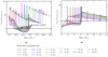 |
Fig. 1. Ratio between mass-loss timescale and lifetime of stars modeled with MESA. Panel a): metallicity = 5 Z⊙. Panel b): metallicity = 9 Z⊙. The horizontal axis shows the total stellar mass, and the vertical axis shows the timescale ratio (see text for more details). The colored tracks show the evolution of the mass-loss timescale for different initial masses (see legend). Stellar evolution starts on the right of the plot and progresses toward the left as mass is lost. The black dashed line is displayed for clarity and shows when the wind-lifetime ratio is equal to one. At a metallicity of 5 Z⊙ (left panel), only systems with M > 13 M⊙ have a wind-lifetime ratio that falls below unity, with varying crossover masses. The panel on the right, at 9 Z⊙, shows that all modeled systems have wind-lifetime ratios that cross below one. The gray shaded oval and the black arrows in the left panel represent the crossover of the wind-lifetime ratio below unity and defines the crossover mass (see Sect. 3 for more details). |
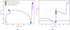 |
Fig. 2. Evolutionary stages of a 15 M⊙ star with 5 Z⊙ modeled with MESA. Panel a): H–R diagram, with key evolutionary points marked with colored stars. Panel b): wind-lifetime ratio vs. mass (one of the tracks from Fig. 1), with the same evolutionary points marked. For this example system (and indeed all other systems), the steepest wind-lifetime ratio decrease occurs when the star halts core H burning and begins He burning. We note that the He burning shown here (marked with the red star) represents the first instance of a decrease in total helium mass, and precedes the core He burning defined in Hurley et al. (2000). |
As seen in Fig. 1a, models with 5 Z⊙ require initial stellar masses of M > 13 M⊙ for the wind-lifetime timescale ratio to dip below one. Conversely, as shown in Fig. 1b, the wind-lifetime timescale ratio of models with 9 Z⊙ across all modeled masses (8 − 22 M⊙) falls below one as the stars transition from hydrogen core burning to helium burning. This indicates that mass loss due to winds is significant for systems at very high metallicities.
The mass at which the timescale ratio equals one is defined as the crossover mass Mcross. If Mcross ≲ 8 M⊙, then the system loses sufficient mass and no longer end its life in a Type II supernova and would therefore fail to further enrich the ISM. We adopted this notion of a crossover mass due to the limitations of MESA in modeling massive stars at high metallicities at more advanced evolutionary stages.
We emphasize that the existence of a crossover mass alone is not sufficient to make conclusions about whether the system undergoes a Type II supernova. The mass value at which crossover occurs must be below 8 M⊙ for the system to no longer undergo a supernova. Thus, the crossover mass value acts as a simple test of whether a star undergoing wind-driven mass loss loses enough mass to avoid a supernova.
Figure 3 shows the crossover mass of all models where the timescale ratio reached below one, for all modeled metallicities. We clearly see that the 3 Z⊙ and 5 Z⊙ systems have Mcross > 8 M⊙, and Type II supernovae and enrichment can continue to occur. Therefore, metallicities below 5 Z⊙ are insufficient to produce a metallicity ceiling.
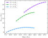 |
Fig. 3. Crossover mass of all modeled systems. The horizontal axis shows the initial mass of the star, and the vertical axis shows the crossover mass, namely the mass at which the mass-loss timescale is shorter than the remaining stellar lifetime (see Fig. 1). Lower-mass stars than those shown for Z = 3 Z⊙ or Z = 5 Z⊙ do not have a crossover mass (see Fig. 1 for Z = 5 Z⊙ example). Stars with Z = 3 Z⊙ or Z = 5 Z⊙ clearly have Mcross ≳ 8 M⊙, while stars with Z = 9 Z⊙ have Mcross ≲ 8 M⊙. This implies that stars forming in a Z = 9 Z⊙ ISM fail to undergo Type II supernovae and lead to a metallicity ceiling in the ISM. |
However, for 9 Z⊙ systems, we see that Mcross ≲ 8 M⊙ for all modeled masses with a decreasing trend toward the higher masses. This indicates that, at very high metallicities of approximately 9 Z⊙, massive stars with M > 8 M⊙ fail to retain enough mass to end their lives as Type II supernovae. Therefore, our model heuristically demonstrates that stars no longer undergo supernovae and cannot further enrich the ISM once the ISM metallicity reaches approximately 9 Z⊙. A metallicity ceiling is thus possible once stars begin to form in a 9 Z⊙ ISM. Taking into account the intrinsic uncertainties of modeling massive stars at high metallicities with wind-driven mass loss, this result is consistent with the observed average BLR metallicity of no more than 9.5 Z⊙ (Simon & Hamann 2010).
4. Additional tests
4.1. Metallicity
Figure 4 explicitly shows the effect of different metallicities on the evolution and crossover mass of a 17 M⊙ star (with a Dutch_scaling_factor = 2). Aside from metallicity, all other model parameters were identical between the three models shown in Fig. 4. It is clear that a higher Z leads to more efficient winds and greater mass loss before the onset of helium burning in the stars (refer to Fig. 2 for evolutionary stages). This can be explained by the direct dependence on Z of the Dutch wind model as well as the effect of Z on other stellar parameters relevant in the wind model (refer to Sect. 2 for wind model references and further details). The crossover masses likewise decrease with increasing Z.
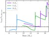 |
Fig. 4. Wind-lifetime ratio vs. mass of a 17 M⊙ star at different metallicities. The axes are the same as those in Fig. 1 and the right panel of Fig. 2. This plot combines the 17 M⊙ tracks previously shown in Fig. 1 (at 5 Z⊙ and 9 Z⊙) with the 3 Z⊙ model. The crossover masses decrease with increasing metallicity (see text). The first 2 million years of evolution have been excluded for plot clarity. |
4.2. Wind model
As mentioned in Sect. 2, we selected a scaling factor of 2.0 for the Dutch wind model. However, since the modeling of massive star evolution at high metallicities using MESA is overall uncertain, we conducted a test with a 25% reduction in the Dutch wind scaling factor on a 12 M⊙ star at 9 Z⊙.
When the Dutch_scaling_factor was set to 2.0, the crossover mass of the system was 7.3 M⊙ (see the blue line in Fig. 3). Since this crossover mass is below the minimum supernova mass of 8 M⊙, the system would not undergo supernovae in its lifetime.
However, when this Dutch_scaling_factor was reduced by 25%, the crossover mass for this 12 M⊙ star at 9 Z⊙ increased to 8.1 M⊙ and therefore the star would undergo supernovae. At first glance, this would seem to suggest that our results are sensitive to the choice of Dutch_scaling_factor. However, this is not the case, since a small increase in metallicity would decrease the crossover mass and compensate for the effect of a lower wind scaling factor. As shown in Fig. 5, an increase in metallicity by 0.5 Z⊙ to a value of 9.5 Z⊙ is sufficient to decrease the crossover mass to 7.2 M⊙ (see green line in Fig. 5). Since the possible metallicity ceiling from Simon & Hamann (2010) has sizable uncertainties, this 0.5 Z⊙ change in metallicity is acceptable. Therefore, the results of this work remain qualitatively valid with changes in the Dutch wind scaling factor.
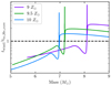 |
Fig. 5. Wind-lifetime ratio vs. mass of a 12 M⊙ star with reduced winds at different metallicities. The axes are the same as those in Fig. 1 and the right panel of Fig. 2. The crossover masses decrease with increasing metallicity (see text). |
5. Discussion and conclusions
We investigated whether stars embedded near quasars (quasar stars) can lead to a metallicity ceiling based on a simple closed box model. We assumed that the stars evolve over many cycles and progressively increase the metallicity within the closed system, and explicitly studied the last cycle of stars that may remain massive enough to evolve and enrich the ISM via Type II supernovae. Observationally, evidence of a metallicity ceiling in quasars was presented in Simon & Hamann (2010), who found a BLR metallicity average of no more than 9.5 Z⊙, with no significant dependence on the SFR.
We evolved stars with masses of 8 − 22 M⊙ and with 3 Z⊙, 5 Z⊙, and 9 Z⊙, using MESA to explore the mass–metallicity parameter space required for a metallicity ceiling. We found that for an existing ISM metallicity of 9 Z⊙, stars with masses of 8 − 22 M⊙ lose enough mass before core helium burning to fall below the ∼8 M⊙ Type II supernova threshold, and they therefore lead to a metallicity ceiling. We determined that lower ISM metallicities of 5 Z⊙ and 3 Z⊙ are insufficient for a metallicity ceiling, and therefore conclude that a minimum ISM metallicity of 9 Z⊙ is needed for saturation of the enrichment process. Consequently, a metallicity ceiling may be a general phenomenon in environments that can be approximated as stellar formation and evolution within a closed box.
The idea of a metallicity ceiling in quasars has implications to our understanding of black hole accretion and nuclear star clusters (NSCs). For instance, stellar formation at the outer regions of quasar disks (Goodman & Tan 2004) may be a possible explanation for periods of lower-than-expected black hole accretion rates, since the gas that would otherwise be accreted instead fragments and forms stars, with the accretion being choked. However, as the metallicity of stars becomes too high to maintain stability after many cycles, gas may no longer be trapped in stars, and thus black hole accretion rates increase to expected levels and choked accretion is lifted. If we adopt the metallicity ceiling idea for star formation in the outer regions of the disk, the changes in the black hole accretion rates may reveal information about the fraction of inflowing gas that reaches the inner accretion disk vs. the fraction that remains in the outer star-forming region.
Additionally, there is an almost-constant ratio between the mass of NSCs and the mass of the central black hole (Neumayer et al. 2020) in observations. If NSCs form with the presence of a metallicity ceiling that lifts choked accretion, this almost-constant ratio of black hole mass and NSC mass may be explained.
The metallicity ceiling discussed in this paper is still valid in binary and multiple stellar systems. Although most massive stars are in binary or multiple-star systems (e.g., Sana et al. 2012), binary interactions would only serve to increase metallicity through mixing, leading to the system reaching a metallicity ceiling more rapidly. As the accretor star gains mass, it experiences stronger winds, losing mass more rapidly than it gains mass (in MESA’s Dutch wind model), therefore becoming more likely to fall below ∼8 M⊙. Likewise, the donor star loses mass and more likely falls below ∼8 M⊙. Therefore, the presence of multiple-star systems would only lead to the system more effectively suppressing supernovae.
Additionally, we can interpret our result through the lens of stellar masses. When supernovae are suppressed, a mass cut-off past the minimum supernova mass of ∼8 M⊙ is expected. Therefore, the presence of a highly super-solar metallicity ceiling of ∼10 Z⊙ suggests a mass cut-off above ∼8 M⊙.
We emphasize that the metallicity ceiling and the suppression of supernovae described in this work applies only to environments that can be approximated as a closed box. For more realistic environments, the inflowing fresh gas is able to maintain Z < 8 Z⊙, allowing for supernovae to occur, and a metallicity ceiling is not present.
The MESA equation of state (EOS) combine OPAL (Rogers & Nayfonov 2002), SCVH (Saumon et al. 1995), FreeEOS (Irwin 2004), HELM (Timmes & Swesty 2000), PC ((Potekhin & Chabrier 2010), and Skye (Jermyn et al. 2021) EOSes. Radiative opacities combine OPAL (Iglesias & Rogers 1993, 1996 and data from Ferguson et al. (2005) and Poutanen (2017). Electron conduction opacities are from Cassisi et al. (2007). Nuclear reaction rates are from JINA REACLIB (Cyburt et al. 2010), NACRE (Angulo et al. 1999), and Fuller et al. (1985), Oda et al. (1994), Langanke & Martínez-Pinedo (2000). Screening is included via the prescription of Chugunov et al. (2007). Thermal neutrino loss rates are from Itoh et al. (1996).
Acknowledgments
We thank Evan Bauer for advice and comments on MESA wind modeling, and Matteo Cantiello, Charlie Conroy, Lars Hernquist, and Mark Reid for helpful comments on the manuscript.
References
- Agrawal, P., Szécsi, D., Stevenson, S., Eldridge, J. J., & Hurley, J. 2022, MNRAS, 512, 5717 [NASA ADS] [CrossRef] [Google Scholar]
- Angulo, C., Arnould, M., Rayet, M., et al. 1999, Nucl. Phys. A, 656, 3 [Google Scholar]
- Antonucci, R. 1993, ARA&A, 31, 473 [Google Scholar]
- Belczynski, K., Romagnolo, A., Olejak, A., et al. 2022, ApJ, 925, 69 [NASA ADS] [CrossRef] [Google Scholar]
- Best, P. N., & Heckman, T. M. 2012, MNRAS, 421, 1569 [NASA ADS] [CrossRef] [Google Scholar]
- Cassisi, S., Potekhin, A. Y., Pietrinferni, A., Catelan, M., & Salaris, M. 2007, ApJ, 661, 1094 [NASA ADS] [CrossRef] [Google Scholar]
- Castor, J. I., Abbott, D. C., & Klein, R. I. 1975, ApJ, 195, 157 [Google Scholar]
- Chugunov, A. I., Dewitt, H. E., & Yakovlev, D. G. 2007, Phys. Rev. D, 76, 025028 [NASA ADS] [CrossRef] [Google Scholar]
- Crowther, P. A., Schnurr, O., Hirschi, R., et al. 2010, MNRAS, 408, 731 [Google Scholar]
- Cyburt, R. H., Amthor, A. M., Ferguson, R., et al. 2010, ApJS, 189, 240 [NASA ADS] [CrossRef] [Google Scholar]
- Dhanda, N., Baldwin, J. A., Bentz, M. C., & Osmer, P. S. 2007, ApJ, 658, 804 [NASA ADS] [CrossRef] [Google Scholar]
- Elitzur, M., & Ho, L. C. 2009, ApJ, 701, L91 [Google Scholar]
- Elvis, M. 2000, ApJ, 545, 63 [NASA ADS] [CrossRef] [Google Scholar]
- Ferguson, J. W., Alexander, D. R., Allard, F., et al. 2005, ApJ, 623, 585 [Google Scholar]
- Fields, C. E., Timmes, F. X., Farmer, R., et al. 2018, ApJS, 234, 19 [NASA ADS] [CrossRef] [Google Scholar]
- Fuller, G. M., Fowler, W. A., & Newman, M. J. 1985, ApJ, 293, 1 [NASA ADS] [CrossRef] [Google Scholar]
- Glebbeek, E., Gaburov, E., de Mink, S. E., Pols, O. R., & Portegies Zwart, S. F. 2009, A&A, 497, 255 [NASA ADS] [CrossRef] [EDP Sciences] [Google Scholar]
- Goldberg, J. A., & Bildsten, L. 2020, ApJ, 895, L45 [CrossRef] [Google Scholar]
- Goldberg, J. A., Bildsten, L., & Paxton, B. 2019, ApJ, 879, 3 [Google Scholar]
- Goodman, J., & Tan, J. C. 2004, ApJ, 608, 108 [NASA ADS] [CrossRef] [Google Scholar]
- Hamann, F., Korista, K. T., Ferland, G. J., Warner, C., & Baldwin, J. 2002, ApJ, 564, 592 [NASA ADS] [CrossRef] [Google Scholar]
- Higgins, E. R., & Vink, J. S. 2020, A&A, 635, A175 [NASA ADS] [CrossRef] [EDP Sciences] [Google Scholar]
- Hurley, J. R., Pols, O. R., & Tout, C. A. 2000, MNRAS, 315, 543 [Google Scholar]
- Iglesias, C. A., & Rogers, F. J. 1993, ApJ, 412, 752 [Google Scholar]
- Iglesias, C. A., & Rogers, F. J. 1996, ApJ, 464, 943 [NASA ADS] [CrossRef] [Google Scholar]
- Irwin, A. W. 2004, Astrophysics Source Code Library [record ascl:1211.002] [Google Scholar]
- Itoh, N., Hayashi, H., Nishikawa, A., & Kohyama, Y. 1996, ApJS, 102, 411 [NASA ADS] [CrossRef] [Google Scholar]
- Izumi, T., Onoue, M., Shirakata, H., et al. 2018, PASJ, 70, 36 [NASA ADS] [Google Scholar]
- Jermyn, A. S., Schwab, J., Bauer, E., Timmes, F. X., & Potekhin, A. Y. 2021, ApJ, 913, 72 [NASA ADS] [CrossRef] [Google Scholar]
- Jiang, L., Fan, X., Vestergaard, M., et al. 2007, AJ, 134, 1150 [NASA ADS] [CrossRef] [Google Scholar]
- Juarez, Y., Maiolino, R., Mujica, R., et al. 2009, A&A, 494, L25 [NASA ADS] [CrossRef] [EDP Sciences] [Google Scholar]
- Krolik, J. H., & Begelman, M. C. 1988, ApJ, 329, 702 [Google Scholar]
- Kudritzki, R.-P., & Puls, J. 2000, ARA&A, 38, 613 [Google Scholar]
- Langanke, K., & Martínez-Pinedo, G. 2000, Nucl. Phys. A, 673, 481 [NASA ADS] [CrossRef] [Google Scholar]
- Lucy, L. B., & Solomon, P. M. 1970, ApJ, 159, 879 [Google Scholar]
- Mignoli, M., Feltre, A., Bongiorno, A., et al. 2019, A&A, 626, A9 [NASA ADS] [CrossRef] [EDP Sciences] [Google Scholar]
- Miniutti, G., Sanfrutos, M., Beuchert, T., et al. 2014, MNRAS, 437, 1776 [NASA ADS] [CrossRef] [Google Scholar]
- Morganti, R. 2017, Front. Astron. Space Sci., 4, 42 [CrossRef] [Google Scholar]
- Müller, A. L., & Romero, G. E. 2020, A&A, 636, A92 [NASA ADS] [CrossRef] [EDP Sciences] [Google Scholar]
- Murray, N., Quataert, E., & Thompson, T. A. 2005, ApJ, 618, 569 [NASA ADS] [CrossRef] [Google Scholar]
- Nagao, T., Marconi, A., & Maiolino, R. 2006, A&A, 447, 157 [NASA ADS] [CrossRef] [EDP Sciences] [Google Scholar]
- Netzer, H. 2015, ARA&A, 53, 365 [Google Scholar]
- Neumayer, N., Seth, A., & Böker, T. 2020, A&ARv, 28, 4 [Google Scholar]
- Ni, Y., Di Matteo, T., Feng, Y., Croft, R. A. C., & Tenneti, A. 2018, MNRAS, 481, 4877 [NASA ADS] [CrossRef] [Google Scholar]
- Nicastro, F. 2000, ApJ, 530, L65 [NASA ADS] [CrossRef] [Google Scholar]
- Nugis, T., & Lamers, H. J. G. L. M. 2000, A&A, 360, 227 [NASA ADS] [Google Scholar]
- Oda, T., Hino, M., Muto, K., Takahara, M., & Sato, K. 1994, Atomic Data and Nuclear Data Tables, 56, 231 [CrossRef] [Google Scholar]
- Paxton, B., Bildsten, L., Dotter, A., et al. 2011, ApJS, 192, 3 [Google Scholar]
- Paxton, B., Cantiello, M., Arras, P., et al. 2013, ApJS, 208, 4 [Google Scholar]
- Paxton, B., Marchant, P., Schwab, J., et al. 2015, ApJS, 220, 15 [Google Scholar]
- Paxton, B., Schwab, J., Bauer, E. B., et al. 2018, ApJS, 234, 34 [NASA ADS] [CrossRef] [Google Scholar]
- Paxton, B., Smolec, R., Schwab, J., et al. 2019, ApJS, 243, 10 [Google Scholar]
- Perna, R., Lazzati, D., & Cantiello, M. 2018, ApJ, 859, 48 [NASA ADS] [CrossRef] [Google Scholar]
- Potekhin, A. Y., & Chabrier, G. 2010, Contrib. Plasma Phys., 50, 82 [NASA ADS] [CrossRef] [Google Scholar]
- Poutanen, J. 2017, ApJ, 835, 119 [NASA ADS] [CrossRef] [Google Scholar]
- Quataert, E., Fernández, R., Kasen, D., Klion, H., & Paxton, B. 2016, MNRAS, 458, 1214 [NASA ADS] [CrossRef] [Google Scholar]
- Rieke, G. H. 1988, ApJ, 331, L5 [NASA ADS] [CrossRef] [Google Scholar]
- Rogers, F. J., & Nayfonov, A. 2002, ApJ, 576, 1064 [Google Scholar]
- Sana, H., de Mink, S. E., de Koter, A., et al. 2012, Science, 337, 444 [Google Scholar]
- Sander, A. A. C., & Vink, J. S. 2020, MNRAS, 499, 873 [Google Scholar]
- Saumon, D., Chabrier, G., & van Horn, H. M. 1995, ApJS, 99, 713 [NASA ADS] [CrossRef] [Google Scholar]
- Shemmer, O., Netzer, H., Maiolino, R., et al. 2004, ApJ, 614, 547 [NASA ADS] [CrossRef] [Google Scholar]
- Shiode, J. H., & Quataert, E. 2014, ApJ, 780, 96 [Google Scholar]
- Simon, L. E., & Hamann, F. 2010, MNRAS, 407, 1826 [NASA ADS] [CrossRef] [Google Scholar]
- Sun, M. 2023, MNRAS, 521, 2954 [NASA ADS] [CrossRef] [Google Scholar]
- Timmes, F. X., & Swesty, F. D. 2000, ApJS, 126, 501 [NASA ADS] [CrossRef] [Google Scholar]
- Trump, J. R., Impey, C. D., Kelly, B. C., et al. 2011, ApJ, 733, 60 [NASA ADS] [CrossRef] [Google Scholar]
- Vink, J. S., de Koter, A., & Lamers, H. J. G. L. M. 2001, A&A, 369, 574 [NASA ADS] [CrossRef] [EDP Sciences] [Google Scholar]
- Vink, J. S., & Sander, A. A. C. 2021, MNRAS, 504, 2051 [NASA ADS] [CrossRef] [Google Scholar]
- Warner, C., Hamann, F., & Dietrich, M. 2003, ApJ, 596, 72 [NASA ADS] [CrossRef] [Google Scholar]
- Warner, C., Hamann, F., & Dietrich, M. 2004, ApJ, 608, 136 [NASA ADS] [CrossRef] [Google Scholar]
All Figures
|
Fig. 1. Ratio between mass-loss timescale and lifetime of stars modeled with MESA. Panel a): metallicity = 5 Z⊙. Panel b): metallicity = 9 Z⊙. The horizontal axis shows the total stellar mass, and the vertical axis shows the timescale ratio (see text for more details). The colored tracks show the evolution of the mass-loss timescale for different initial masses (see legend). Stellar evolution starts on the right of the plot and progresses toward the left as mass is lost. The black dashed line is displayed for clarity and shows when the wind-lifetime ratio is equal to one. At a metallicity of 5 Z⊙ (left panel), only systems with M > 13 M⊙ have a wind-lifetime ratio that falls below unity, with varying crossover masses. The panel on the right, at 9 Z⊙, shows that all modeled systems have wind-lifetime ratios that cross below one. The gray shaded oval and the black arrows in the left panel represent the crossover of the wind-lifetime ratio below unity and defines the crossover mass (see Sect. 3 for more details). |
| In the text | |
|
Fig. 2. Evolutionary stages of a 15 M⊙ star with 5 Z⊙ modeled with MESA. Panel a): H–R diagram, with key evolutionary points marked with colored stars. Panel b): wind-lifetime ratio vs. mass (one of the tracks from Fig. 1), with the same evolutionary points marked. For this example system (and indeed all other systems), the steepest wind-lifetime ratio decrease occurs when the star halts core H burning and begins He burning. We note that the He burning shown here (marked with the red star) represents the first instance of a decrease in total helium mass, and precedes the core He burning defined in Hurley et al. (2000). |
| In the text | |
|
Fig. 3. Crossover mass of all modeled systems. The horizontal axis shows the initial mass of the star, and the vertical axis shows the crossover mass, namely the mass at which the mass-loss timescale is shorter than the remaining stellar lifetime (see Fig. 1). Lower-mass stars than those shown for Z = 3 Z⊙ or Z = 5 Z⊙ do not have a crossover mass (see Fig. 1 for Z = 5 Z⊙ example). Stars with Z = 3 Z⊙ or Z = 5 Z⊙ clearly have Mcross ≳ 8 M⊙, while stars with Z = 9 Z⊙ have Mcross ≲ 8 M⊙. This implies that stars forming in a Z = 9 Z⊙ ISM fail to undergo Type II supernovae and lead to a metallicity ceiling in the ISM. |
| In the text | |
|
Fig. 4. Wind-lifetime ratio vs. mass of a 17 M⊙ star at different metallicities. The axes are the same as those in Fig. 1 and the right panel of Fig. 2. This plot combines the 17 M⊙ tracks previously shown in Fig. 1 (at 5 Z⊙ and 9 Z⊙) with the 3 Z⊙ model. The crossover masses decrease with increasing metallicity (see text). The first 2 million years of evolution have been excluded for plot clarity. |
| In the text | |
|
Fig. 5. Wind-lifetime ratio vs. mass of a 12 M⊙ star with reduced winds at different metallicities. The axes are the same as those in Fig. 1 and the right panel of Fig. 2. The crossover masses decrease with increasing metallicity (see text). |
| In the text | |
Current usage metrics show cumulative count of Article Views (full-text article views including HTML views, PDF and ePub downloads, according to the available data) and Abstracts Views on Vision4Press platform.
Data correspond to usage on the plateform after 2015. The current usage metrics is available 48-96 hours after online publication and is updated daily on week days.
Initial download of the metrics may take a while.