| Issue |
A&A
Volume 678, October 2023
|
|
|---|---|---|
| Article Number | A13 | |
| Number of page(s) | 9 | |
| Section | Cosmology (including clusters of galaxies) | |
| DOI | https://doi.org/10.1051/0004-6361/202346236 | |
| Published online | 28 September 2023 | |
Nonparametric analysis of the Hubble diagram with neural networks
1
Dipartimento di Fisica e Astronomia, Università di Firenze, Via G. Sansone 1, 50019 Sesto Fiorentino, Firenze, Italy
e-mail: lorenzo.giambagli@unifi.it
2
naXys – Namur Center for Complex Systems, University of Namur, Rue Grafé 2, 5000 Namur, Belgium
3
INFN and CSDC, Via Sansone 1, 50019 Sesto Fiorentino, Firenze, Italy
4
INAF – Osservatorio Astrofisico di Arcetri, Largo Enrico Fermi 5, 50125 Firenze, Italy
Received:
24
February
2023
Accepted:
10
July
2023
The recent extension of the Hubble diagram of supernovae and quasars to redshifts much higher than 1 prompted a revived interest in nonparametric approaches to test cosmological models and to measure the expansion rate of the Universe. In particular, it is of great interest to infer model-independent constraints on the possible evolution of the dark energy component. Here we present a new method, based on neural network regression, to analyze the Hubble diagram in a completely nonparametric, model-independent fashion. We first validated the method through simulated samples with the same redshift distribution as the real ones, and we discuss the limitations related to the “inversion problem” for the distance-redshift relation. We then applied this new technique to the analysis of the Hubble diagram of supernovae and quasars. We confirm that the data up to z ∼ 1 − 1.5 are in agreement with a flat Λ cold dark matter model with ΩM ∼ 0.3, while ∼5-sigma deviations emerge at higher redshifts. A flat Λ cold dark matter model would still be compatible with the data with ΩM > 0.4. Allowing for a generic evolution of the dark energy component, we find solutions that suggest an increasing value of ΩM with redshift, as predicted by interacting dark sector models.
Key words: methods: data analysis / methods: analytical / cosmological parameters
© The Authors 2023
 Open Access article, published by EDP Sciences, under the terms of the Creative Commons Attribution License (https://creativecommons.org/licenses/by/4.0), which permits unrestricted use, distribution, and reproduction in any medium, provided the original work is properly cited.
This article is published in open access under the Subscribe to Open model. Subscribe to A&A to support open access publication.
1. Introduction
The Hubble diagram (i.e., the distance-redshift relation) describes the expansion of the Universe with time and is one of the fundamental tools of observational cosmology. The “kinematic” information encoded in this diagram includes the Hubble parameter H0 (from the first-order derivative at redshift z = 0) and the acceleration parameter (from the second-order derivative). When a dynamical model is adopted, its physical parameters can be derived from the fit of the Hubble diagram. Typical examples are the estimate of the matter density at z = 0, ΩM, within a flat Λ cold dark matter (CDM) model, or the evaluation of ΩM and ΩΛ within a non-flat ΛCDM model. Moreover, the physical meaning of the relevant parameters to some extent reflects the chosen model. Likewise, the obtained numerical estimates are also model-dependent: if we assume, for example, that data follow a ΛCDM model, with prescribed ΩM and nonzero curvature, it is easy to demonstrate through numerical simulations that, if a flat ΛCDM is adopted, the best-fit value of ΩM will be different from the correct (simulated) one.
In the past few years, possible new physics beyond the flat ΛCDM model has been suggested by several observational results, such as the mismatch between the direct measurements of H0 in the local Universe (Riess et al. 2019; Wong et al. 2019) and the extrapolations based on the cosmic microwave background, the comparison between the high- and low- multipole spectra of the cosmic microwave background (Di Valentino et al. 2021), and the tension between the power spectrum of density perturbations measured on different scales (Macaulay et al. 2013; Battye et al. 2015; Lin & Ishak 2017; Heymans et al. 2021; Nunes & Vagnozzi 2021). Recently, a significant deviation from the flat ΛCDM model has been observed in the Hubble diagram at high redshifts, an area populated with quasars and γ-ray bursts: while no significant tension is found at z < 1.5 with supernovae, quasars, or γ-ray bursts, the data at z > 1.5 suggest a slower expansion of the Universe than predicted by the flat ΛCDM model (Risaliti & Lusso 2019; Demianski et al. 2017; Lusso et al. 2019, 2020). These results make it particularly important to analyze the Hubble diagram in a way that is as model-agnostic as possible, in order to obtain an “absolute scale” for the comparison with specific models, and to infer the global, “cosmographic” properties of the expansion, which, in turn, could suggest the optimal class of model to fit to the data.
Cosmographic expansions (Aviles et al. 2014; Capozziello et al. 2020; Bargiacchi et al. 2021) represent a viable approach to achieving this goal. The method is based on a standard fitting procedure and assumes that observational data can be interpolated by an appropriate series of functions, truncated to include a limited number of terms (and hence a limited number of free parameters). While this is not dependent on a specific physical model, it still relies on the flexibility of the chosen functions to reproduce the shape of the observational Hubble diagram. Moreover, cosmographic techniques are rigorously valid only within a convergence radius, which is z = 1 for standard methods (Cattoën & Visser 2007). At higher redshifts, no method has an absolute validity based on mathematical principles, and the effectiveness of the cosmographic analysis relies on the similarity between the chosen expansion functions and the actual shape of Hubble diagram.
An example of a robust, well-checked, nonparametric approach is that based on Gaussian process (GP) regression (Holsclaw et al. 2010; Seikel et al. 2012; Shafieloo et al. 2012), which has been used to test the hypothesis of a constant density of the dark energy term (i.e., the cosmological constant Λ). Despite their flexibility, however, GPs may underestimate the error associated with predictions (Colgáin 2021) and come with an intrinsic convergence problem for z > 1.
Starting from these premises, we here propose, and consequently apply, a novel analysis framework for the Hubble diagram based on neural network (NN) regression (see Dialektopoulos et al. 2022 for a similar approach). Deep feed-forward fully connected NNs are well-known universal approximators. Their ability to represent functions extends far beyond what is required for the particular problem at hand. However, the core of their efficacy lies in the assumption that the proper regression function results from a collection of several multilevel hierarchical factors (or features) that could enable one to account for unknown features in the analysis that bear – at least some – cosmological relevance. To sum up, we try to merge the concept of features with cascading relevance appropriate for cosmographic expansion with the need for convergence and the high-function representation capabilities typical of kernel methods or GPs.
We first describe the method and check its reliability with simulated data sets. Then we apply it to a Hubble diagram at high redshifts, showing a high-redshift inconsistency with the ΛCDM model. Finally, we speculate on the class of model that could fix the discrepancy.
2. The cosmological background
In a Friedmann–Robertson–Walker Universe, the luminosity distance of an astrophysical source is related to the redshift through the equation
where H(z) is the Hubble function and ΩK stands for the curvature parameter, defined as ΩK = 1 − ∑iΩi, with Ωi representing the density of the constituents of the Universe, normalized to the closure density. In the simplest form – assuming a flat Universe, a constant total content of matter in the Universe, and a cosmological constant and considering the redshift range where standard candles are observed (i.e., z < 7, where the contribution of the radiation and neutrino terms is negligible) –  . However, a wide range of different physical and cosmological models have been considered in the literature, including a nonzero curvature, an evolving dark energy density, and/or interactions between dark energy and dark matter. In this work, we analyze a subset of these models, represented by the equation
where w(z) is a generic redshift evolution of the dark energy component density. Our main goal is to test the consistency of the flat ΛCDM hypothesis (which amounts to setting w = −1 in Eq. (2)) with the present Hubble diagram of supernovae and quasars, and draw a comparison with other possible functional forms for w(z), as proposed in the literature. To this aim, we carried out a nonparametric fit via a suitably designed NN. This enabled us to reach conclusions on the predicted profile of w(z) without relying on any a priori assumption.
One key problem in any nonparametric reconstruction attempt is the so-called inversion problem: it is easy to demonstrate that the inversion of Eq. (2), which involves the first and second derivatives of H(z) (see, e.g., Seikel et al. 2012), is inherently unstable, due to a strong dependence on the ΩM and H0 parameters; in particular, a change in the quantity  by as little as 0.1% can alter the predicted value of w(z) by orders of magnitude and/or flip its sign. As a consequence, constraints on w(z) at very low redshifts can be obtained, but the uncertainties become very large beginning at z ∼ 0.5. This makes it difficult to reach hard conclusions about the supposed consistency of available data with the reference scenario with w = −1. In principle, better data could help reduce the uncertainties. While we will discuss this issue in more detail in a dedicated paper, here we just mention the relevant point for the present work: it is not possible to obtain significant information on w(z) from the Hubble diagram without (a) assuming some analytic form of the function and/or (b) having a combined estimate of ΩM and H0 with a much higher precision than what is available today and in the foreseeable future. There are only two possible direct ways to overcome this limitation: either we restrict our analysis to very narrow ranges of the parameters, or we constrain the shape of the function w(z). Since neither of these approaches is satisfactory (and both have already been explored in the literature), we chose a different strategy. We did not attempt to carry out a full inversion of Eq. (2). On the contrary, we overcame the aforementioned numerical problems by estimating the quantity
which can be determined from the observational data by solely invoking the first derivative of H(z) (see Cárdenas 2015 for an early application of this technique). We notice that within the ΛCDM model, w = −1 implies I(z) = 0. As an obvious limitation, we will just recover the integral of the physical quantity of interest, the function w(z): the degeneracy on w(z) implies that different forms of w(z) lead to indistinguishable shapes of I(z). Nonetheless, we can achieve some remarkable results. First, we can compare the results on I(z) with the prediction of the flat ΛCDM model: an inconsistency here would be powerful and general proof of a tension between the model and the data (note that the opposite is not true: an agreement based on the analysis of I(z) does not necessarily imply an invalidation of the ΛCDM model). More generally, we can explore the family of w(z) functions that lead to the observation-based reconstruction of I(z) to determine which class of physical model can reproduce the observed Hubble diagram.
3. Regression via deep neural networks
For our purposes we have chosen to deal with a fully connected feed-forward architecture, as illustrated in the supplementary information (SI) Appendix B. Function (3) is hence approximated by a suitable NN, denoted as INN, to be determined via the following apposite optimization procedure. After a few manipulations, as detailed in the SI, the data set takes the form 𝒟 = {(z(i), y(i), Δy(i))} with i ∈ 1…|𝒟|, where y(i) is connected to the modulus of luminosity distance,  , and Δy(i) stands for the associated empirical error. The predictions,
  and the supplied input, y(i), are linked via
![$$ \begin{aligned} { y}_{\text{pred}}^{(i)} = \int _{0}^{z^{(i)}}\mathrm{d}z^\prime \left[\Omega _{\rm M}\left(1+z^\prime \right)^3+\left(1-\Omega _{\rm M}\right)\mathrm{e}^{3I_{\rm NN}(z^\prime )}\right]^{-\frac{1}{2}} .\end{aligned} $$](/articles/aa/full_html/2023/10/aa46236-23/aa46236-23-eq8.gif)
We note that the prediction is a functional of INN, the NN approximation that constitutes the target of the analysis. To carry out the optimization, we introduced the loss function  . The weights of the network that ultimately defines INN are tuned so as to minimize the above loss function via conventional stochastic gradient descent (SGD) methods. The hyperparameters were optimized with mock data samples, as illustrated in the SI. To quantify the statistical errors Δypred (associated with the predictions) and ΔINN (referring to the approximating NN), we implemented a bootstrap procedure, which is detailed in the SI. The code is freely available online1.
This regression scheme was tested against a selection of mock data samples. In carrying out the test we considered:
(A) A sample of 4000 sources with no dispersion, with a flat distribution in log(z) between z = 0.01 and z = 6, and following a flat ΛCDM model with ΩM = 0.3 and h = H0/(100 km s−1 Mpc−1) = 0.7. This sample (as well as the next on the list) represents a highly idealized, hence unrealistic, setting. It is solely used as a reference benchmark model for preliminary consistency checks.
(B) The same as above, but the model used is a Chevallier–Polarski–Linder (CPL) parametrization, which assumes a dark energy equation of state that varies with the redshift as  (Chevallier & Polarski 2001), with w0 = −1.5 and wa = 0.5. We note that this choice of the parameters would be hard to justify from a physical point of view. In particular, it implies a turning point in the Hubble parameter H(z), which violates the null-energy condition. However, even if this scenario can be considered unphysical, it serves our purpose of testing our regression method with extreme models.
(C) A sample with the same size, redshift distribution, and dispersion as the Pantheon supernova Ia sample (Scolnic et al. 2018), assuming a flat ΛCDM model with ΩM = 0.3.
(D) A Pantheon-like sample, as above, but assuming a CPL model with w0 = −1.5 and wa = 0.5.
(E) A sample with the same size and redshift distribution as the combined Pantheon (Scolnic et al. 2018) and quasar (Lusso et al. 2020) samples. The quasar sample consists of 2244 sources with redshifts in the z = 0.5 − 7.5 range (the whole Lusso et al. 2020 sample contains 2421 objects, but the 178 ones at redshift z < 0.5 are not considered in this analysis). We assumed the same dispersion as in the real sample and a flat ΛCDM model with ΩM = 0.3.
(F) The same as setting (E) but assuming a CPL model with w0 = −1.5 and wa = 0.5.
More specifically, we generated synthetic data following these different recipes. The regression scheme, as implemented via the NN, enables us to solve an inverse problem, from the data back to the underlying physical model. The correspondence between postulated and reconstructed physical instances readily translates to a reliable metric for gauging the performance of the proposed procedure, in a fully controllable environment and prior to being applied to the experimental data set. The analysis of settings A and B is discussed in the SI and confirms that our NN method can consistently recover the “true” model and parameters with simulated data of (unrealistic) high quality.
The outcome of the analysis for settings C (top left), D (top right), E (bottom left), and F (bottom right) is displayed in Fig. 1. Both INN(z) (the NN approximation for I(z)) and ypred(z) are represented as a function of the redshift, z. For settings E and F, the associated mean loss is also plotted against the parameter ΩM, which can be freely modulated to explore different scenarios. Working with a data set of type C cannot yield definite conclusions: the NN is unable to recover the correct value of ΩM because different ΛCDM models (INN(z)≃0, within the explored range) provide an equally accurate interpolation of the (simulated) data within statistical errors. The above degeneracy is, however, removed when extending the examined sample so as to include quasars (see the bottom-left panel of Fig. 1, which shows data set E). In this case, the minimum displayed by the loss function points to ΩM = 0.3, the value assumed in the simulations; the corresponding function INN(z) is approximately equal to zero (green shadowed domain) within the errors, which is at variance with what is found by employing the other chosen values of ΩM. Data sets D and F (rightmost panels in Fig. 1) return similar conclusions when operating with data generated according to a CPL prescription. Working with supernovae (over a limited range in z) does not allow us to distinguish between the ΛCDM and CPL model, while the underlying model, assumed for data generation, is correctly singled out when quasars are accounted for (green shadowed region that encloses the dashed line, which represents the exact profile), that is, when extending the data set to higher redshifts. Overall, our results from working on synthetic data suggest that (a) the regression method is reliable and (b) with the current Hubble diagram of supernovae, it is not possible to test the ΛCDM model against possible extensions, such as the CPL model with “phantom-like” dark energy. Such a degeneracy is removed with a combined supernova+quasar sample extending up to z ∼ 7.
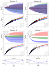 |
Fig. 1. I(z) Results of the NN analysis of the Hubble diagram of simulated data. Top left: data set C, with the same redshift distribution and dispersion as the Pantheon supernova sample. Bottom left: data set E, where combined Pantheon and quasars are considered. In this case, the NN is able to identify the model assumed for data generation (the green shadowed region contains the exact profile for INN(z), depicted with a dashed line). The corresponding loss function is also shown and displays a minimum at the correct value of ΩM. Top right: Pantheon-like sample assumed for a CPL generative model (data set E). The NN is unable to distinguish between different scenarios (ΛCDM vs. CPL). Bottom right: CPL model with the inclusion of quasars. The degeneracy is resolved, and the NN can correctly identify the underlying model (see the dashed line). The loss shows a minimum for the correct value of ΩM, which yields the green shadowed solution for INN(z) vs. z. |
Motivated by the outcome of these simulations, we applied the NN to the experimental data set consisting of the Pantheon supernova sample and the Lusso et al. (2020) quasar sample. The quasar luminosity distances and their errors are estimated from the observational data (X-ray and UV fluxes) following the procedure described in Lusso et al. (2020). In summary, the X-ray and UV data are first fitted in narrow redshift bins in order to derive a cosmology-independent slope, α, of the X-ray to UV relation. This value and its uncertainty are used to derive luminosity distances on an arbitrary scale. The absolute calibration, β, was obtained from the cross-match of the quasar and supernova sample in the common redshift interval. This calibration has a negligible uncertainty with respect to the other components on the error on the luminosity distances: the flux measurement errors, the intrinsic dispersion of the relation, and the error on the slope. In principle, rather than fitting the so-derived luminosity distances, it would be preferable to use the observables (i.e., the fluxes) and to marginalize over the parameters α and β. In practice, the two methods provide identical results, and the use of luminosity distances and Eq. (4) makes the analysis much faster and easier to implement within a NN method.
The results of the NN-based fits are shown in Fig. 2. The shape of I(z) is clearly not consistent with the flat ΛCDM model (I(z)≡0). This is the main result of our work, which we arrived at without assuming any a priori knowledge on the function I(z).
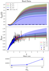 |
Fig. 2. Results of the NN analysis of the Hubble diagram of supernovae (blue points in the middle panel) and quasars (red points). Top panel: estimated values of I(z) for different values of ΩM. Central panel: Hubble diagram with the reconstructed best-fit function obtained from the NN analysis. Bottom panel: Loss values for different values of ΩM. Notice that the solution visually closer (accounting for statistical errors) to the reference ΛCDM profile yields a significantly larger loss value and, as such, should be disregarded. The Loss is indeed nearly flat for ΩM < 0.3. |
As a next step, we introduced a dedicated indicator to quantitatively measure the compatibility of the examined data with the reference ΛCDM model. We naively accessed the distance of the fitted profile, ypred, to the reference yΛCDM (I = 0) curve and divided it by the error associated with the fitted function Δypred. Assuming that the computed ratio (averaged over z) is smaller than the unit, the distance between ypred and yΛCDM is eclipsed by statistical uncertainty and thus ΛCDM cannot be ruled out as a candidate explanatory model. The above procedure has been verified (see the SI) and yields a scalar indicator that fulfills the purpose of quantifying the sought distance, normalized to the associated error. This is denoted by ΔΛCDM and takes the form
The fitted integral function INN is deemed compatible with the ΛCDM model if ΔΛCDM < 1. When this condition holds true, the predictions deviate from ΛCDM by an amount that, on average, is smaller than the corresponding prediction error. The indicator in Eq. (5) was computed for different mock samples, mimicking ΛCDM, with progressively increasing errors sizes, Δy. This error size is assumed uniform across data points and varied from zero to 0.15, thus including the value that is believed to apply to real data: ∼0.14. This information is used as a reference benchmark to interpret the results of the analysis for the Pantheon + quasar experimental data set. To sum up our conclusions (see the SI), the portion of the data set at low redshifts is compatible with a ΛCDM model with Ωm = 0.3, within statistical errors. Conversely, for z > 2 (notably quasars), ΔΛCDM, as computed after available experiments, is 5σ from the expected mean value. Hence, accounting for quasars enables us to conclude that the ΛCDM model is indeed extremely unlikely.
Figure 3 depicts the results where the best-fit I(z) for ΩM = 0.3 (the same as in the upper panel of Fig. 2) is plotted in logarithmic scale and compared to IMATTER(z) = log(z), the function obtained from Eq. (3) by assuming w(z)≡0 (i.e., a pure matter contribution). We recall that a cosmological constant, or equivalently a dark energy component with constant energy, implies w(z)≡ − 1 and I(z)≡0. It is therefore tempting to speculate as follows when qualitatively analyzing the profile of I(z): the redshift intervals with negative derivative represent a dark energy component with density increasing over time (the “phantom” dark energy scenario); the intervals with positive derivatives, smaller than the constant derivative of IMATTER(z), represent a dark energy component with decreasing density; last, the intervals where the derivative is larger than that displayed by IMATTER(z) are matter terms, with increasing density. The prior-free NN solution suggests therefore an “interacting dark sector” scenario, where a matter component decreases with time and, correspondingly, a dark energy component rises. This interpretation is also consistent with the nearly constant loss function for ΩM < 0.3: choosing values larger than 0.3 worsens the agreement because this amounts to overestimating the total matter component at z ∼ 0. Values smaller than 0.3 can be compensated for by the matter component in I(z). This interpretation is consistent with recent claims of an increasing value of ΩM with redshift within a ΛCDM scenario (e.g., Colgáin et al. 2022).
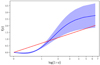 |
Fig. 3. Best-fit I(z) from our NN regression (as in the upper panel of Fig. 2) in logarithmic scale, compared with the function IMATTER(z) obtained by assuming w(z)≡0 in Eq. (3). The redshift intervals where the derivative of I(z) is higher than that of IMATTER(z) represent “matter-like” contributions, while intervals with a lower derivative refer to energy-like contributions. |
4. Conclusions
Our conclusions are multifold. We have proposed and rigorously tested a NN approach for analyzing the Hubble diagram. The NN model-agnostic regression of the combined supernova and quasar catalog enables us to unequivocally reveal a strong tension with the “concordance” flat ΛCDM model. Finally, the analysis we carried out with the proposed NN approach suggests an “interacting dark sector” scenario, where a dark matter component flows into dark energy, at least down to redshifts z ∼ 1.5.
Acknowledgments
We acknowledge financial contribution from the agreement ASI-INAF n.2017-14-H.O. EL acknowledges the support of grant ID: 45780 Fondazione Cassa di Risparmio Firenze. FS acknowledges is financially supported by the National Operative Program (Programma Operativo Nazionale–PON) of the Italian Ministry of University and Research “Research and Innovation 2014–2020”, Project Proposals CIR01_00010. A sincere acknowledgement goes to Dr. Colasurdo, who first performed the data reduction of the LBT KS spectra in her master thesis and developed the baseline analysis that we used as a benchmark. We also acknowledge Prof. Trakhtenbrot for kindly sharing the BASS data.
References
- Aviles, A., Bravetti, A., Capozziello, S., & Luongo, O. 2014, Phys. Rev. D, 90, 043531 [NASA ADS] [CrossRef] [Google Scholar]
- Bargiacchi, G., Risaliti, G., Benetti, M., et al. 2021, A&A, 649, A65 [NASA ADS] [CrossRef] [EDP Sciences] [Google Scholar]
- Battye, R. A., Charnock, T., & Moss, A. 2015, Phys. Rev. D, 91, 103508 [NASA ADS] [CrossRef] [Google Scholar]
- Capozziello, S., D’Agostino, R., & Luongo, O. 2020, MNRAS, 494, 2576 [NASA ADS] [CrossRef] [Google Scholar]
- Cárdenas, V. H. 2015, Phys. Lett. B, 750, 128 [CrossRef] [Google Scholar]
- Cattoën, C., & Visser, M. 2007, Class. Quant. Grav., 24, 5985 [CrossRef] [Google Scholar]
- Chevallier, M., & Polarski, D. 2001, Int. J. Mod. Phys. D, 10, 213 [Google Scholar]
- Colgáin, E., Sheikh-Jabbari, M. M., Solomon, R., Dainotti, M. G., & Stojkovic, D. 2022, arXiv e-prints [arXiv:2206.11447] [Google Scholar]
- Demianski, M., Piedipalumbo, E., Sawant, D., & Amati, L. 2017, A&A, 598, A112 [NASA ADS] [CrossRef] [EDP Sciences] [Google Scholar]
- Di Valentino, E., Melchiorri, A., & Silk, J. 2021, ApJ, 908, L9 [NASA ADS] [CrossRef] [Google Scholar]
- Dialektopoulos, K., Said, J. L., Mifsud, J., Sultana, J., & Zarb Adami, K. 2022, J. Cosmol. Astropart. Phys., 2022, 023 [CrossRef] [Google Scholar]
- Heymans, C., Tröster, T., Asgari, M., et al. 2021, A&A, 646, A140 [NASA ADS] [CrossRef] [EDP Sciences] [Google Scholar]
- Holsclaw, T., Alam, U., Sansó, B., et al. 2010, Phys. Rev. D, 82, 103502 [CrossRef] [Google Scholar]
- Liaw, R., Liang, E., Nishihara, R., et al. 2018, arXiv e-prints [arXiv:1807.05118] [Google Scholar]
- Lin, W., & Ishak, M. 2017, Phys. Rev. D, 96, 023532 [NASA ADS] [CrossRef] [Google Scholar]
- Lusso, E., Piedipalumbo, E., Risaliti, G., et al. 2019, A&A, 628, L4 [NASA ADS] [CrossRef] [EDP Sciences] [Google Scholar]
- Lusso, E., Risaliti, G., Nardini, E., et al. 2020, A&A, 642, A150 [NASA ADS] [CrossRef] [EDP Sciences] [Google Scholar]
- Macaulay, E., Wehus, I. K., & Eriksen, H. K. 2013, Phys. Rev. Lett., 111, 161301 [CrossRef] [Google Scholar]
- Nunes, R. C., & Vagnozzi, S. 2021, MNRAS, 505, 5427 [NASA ADS] [CrossRef] [Google Scholar]
- Colgáin, Ó. E., & Sheikh-Jabbari, M. M. 2021, Eur. Phys. J. C, 81, 892 [CrossRef] [Google Scholar]
- Riess, A. G., Casertano, S., Yuan, W., Macri, L. M., & Scolnic, D. 2019, ApJ, 876, 85 [Google Scholar]
- Risaliti, G., & Lusso, E. 2019, Nat. Astron., 195 [Google Scholar]
- Scolnic, D. M., Jones, D. O., Rest, A., et al. 2018, ApJ, 859, 101 [NASA ADS] [CrossRef] [Google Scholar]
- Seikel, M., Clarkson, C., & Smith, M. 2012, J. Cosmol. Astropart. Phys., 06, 036 [CrossRef] [Google Scholar]
- Shafieloo, A., Kim, A. G., & Linder, E. V. 2012, Phys. Rev. D, 85, 123530 [CrossRef] [Google Scholar]
- Wong, K. C., Suyu, S. H., Chen, G., et al. 2019, MNRAS, 498, 1420 [Google Scholar]
Appendix A: Data processing
Data come as a set 𝒟 = {(z(i), y(i), Δy(i))}, with i ∈ 1…|𝒟|. Each y(i) component is linked to dL, the physical quantity of interest, as  pc). The first applied transformation is defined as follows:

As such, data are traced back to the logarithm of the luminosity distance; every entry of the inspected data set is equal to  .
.
Carrying out a first-order expansion of Eq. (1) in the main body of the paper, assuming a flat Universe (Ωk ∼ 0) and inserting the expression of H(z) as reported in the main text, yields
![$$ \begin{aligned} d_L=\alpha (z)\int _{0}^{z}dz^{\prime }\left[\Omega _M\left(1+z^{\prime }\right)^3+\left(1-\Omega _M\right)e^{I(z^{\prime })}\right]^{-\frac{1}{2}} ,\end{aligned} $$](/articles/aa/full_html/2023/10/aa46236-23/aa46236-23-eq15.gif)
where  . We proceeded by setting

It is worth noting that the relative errors associated with c, z, and H0 are negligible. Relation A.3 transforms into

To simplify the notation, we drop the apex by setting y‴→y and obtain the sought connection between every y(i) and the function to be fitted I(z), namely
![$$ \begin{aligned} y^{(i)} = \int _{0}^{z^{(i)}}dz^{\prime }\left[\Omega _M\left(1+z^{\prime }\right)^3+\left(1-\Omega _M\right)e^{I(z^{\prime })}\right]^{-\frac{1}{2}} .\end{aligned} $$](/articles/aa/full_html/2023/10/aa46236-23/aa46236-23-eq19.gif)
We point out that since arg minxf(x) = arg minxC ⋅ f(x), every manipulation that results in a constant factor in front of the loss function can be ignored. This is the case of every operation in the form of  , which, indeed, results in a factor
  in front of the loss function (see Eq. (C.1)).
Appendix B: The employed neural network model
To approximate the nonlinear scalar function I(z):z ∈ ℝ ↦ I(z)∈ℝ, we made use of a so-called feed-forward architecture. The information flows from the input neuron, associated with z(i), to the output neuron, where the predicted value of INN(z(i)) is displayed.
The transformation from layer k to its adjacent homolog, k + 1, following a feed-forward arrangement, is characterized by two nested operations – (i) a linear map W(k) : ℝNk → ℝNk + 1 and (ii) a nonlinear filter σ(k + 1)(⋅) – applied to each entry of the obtained vector. Here k ranges in the interval 1…ℓ, where N1 = 1 and ℓ is the number of layers (i.e., the depth of the NN). We have chosen σ(k) := tanh for all k < ℓ − 1, whereas σ(ℓ) = 𝕀.
The activation of every neuron in layer k can be consequently obtained as

Furthermore, we fixed Nk = Nk + 1 ∀k ∈ 2…ℓ − 2, meaning that every layer (except the first and the last) has the same size as the others. The size of the so-called hidden layer, N2, and the total amount of layers, ℓ, are, consequently, the only hyperparameters to eventually be fixed.
Occasionally, a neuron-specific scalar, called bias, can be added after the application of each linear map, W(k). To allow for the solution INN(0) = 0 to be recovered, we set the bias to zero.
The output INN(z) hence depends on  free scalar parameters (the weights
  ), which constitute the target of the optimization.
Appendix C: Model optimization
The optimization described in this section was carried out by using parallel computing on GPUs (Liaw et al. 2018) and the minimization of the loss function as defined in the main text was performed via a variant of the SGD method, recalled below. First, data set 𝒟 is shuffled and divided into smaller subsets, ℬi, of size |ℬi|=β. These are the batches, and they meet the following condition:  . Obviously, the number of batches, Nb, is equal to
  . The gradient with respect to every weight, W, entering the definition of the function L is computed, within each batch, as
While i takes values in the range 1…Nb, the weights, W, are updated so as to minimize, via a stochastic procedure, the loss function. This is achieved as follows:
The hyperparameter αlr is called the learning rate and drives the amount of stochasticity in the loss descent process. In the present work a more complex, yet conceptually equivalent, variant of the SGD called Adam is implemented.
A so-called epoch is completed when all batches have been used. The number of epochs, Ne, is another hyperparameter that has to be fixed a priori, as does the batch size, bs. A high number of epochs (such as 400 or 600, as employed in the present application) is usually chosen. To avoid overfitting, the early stop technique is employed. Such a technical aid consists in taking a small subset, 𝒱, of the data set (∼15% of 𝒟) and excluding it from the training process. During training stages, hence, the employed data set is 𝒟′=𝒟 − 𝒱. While applying SGD to the loss so as to minimize it, loss evaluation on data set 𝒱, L(INN, 𝒱) is also performed. When the latter function reaches a plateau, the optimization process is stopped. This procedure relies on two hyperparameters – δ, the absolute variation in L that can be considered a real loss change, and p, the number of consecutive epochs with no recorded variation before the fitting algorithm can eventually be terminated.
One additional hyperparameter needs to be mentioned: as already explained in the main body of the paper, the prediction ypred involves a numerical integral of the NN approximating function, INN. The integration step dz′ thus has to be set and underwent of a meticulous optimization. A hyper-optimization process designed to find the best set of hyperparameters was carried out, employing several CPL- and ΛCDM-like models. Such a process resulted in a set of parameters that were fixed and left unchanged during the trials. A list of the chosen hyperparameters is provided in Table C.1.
Hyperparameters employed.
Appendix D: Simulation results
In the following we report the results of the regression model against the simulated settings mentioned, but not displayed, in the main text.
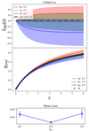 |
Fig. D.1. Simulations with a "perfect" sample (data set A): results of the NN analysis of a simulated sample of 4,000 objects with a log-flat redshift distribution and a negligible dispersion with respect to a flat ΛCDM model with ΩM = 0.3. Top panel: Estimated values of I(z) for different values of ΩM (Eq. 3; the "correct" value for the simulated data is I(z)≡0). Central panel: Hubble diagram with the reconstructed best-fit function obtained from the NN analysis. Bottom panel: Loss values for different values of ΩM. The minimum is at ΩM = 0.3, i.e., the "true" value. The corresponding I(z) is consistent with zero at all redshifts. These results demonstrate that the NN analysis is able to recover the correct model and the "true"value of ΩM. |
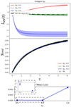 |
Fig. D.2. Results for data set B. The governing model is a CPL with w0 = −1.5, wa = 0.5. |
Appendix E: Estimating the errors
To estimate the prediction error Δypred(z), we employed a bootstrap method. To this end, the fitting procedure was arranged so as to produce B independent estimators of the quantity ypred and INN(z), namely ![$ y_\text{pred}^{[k]} $](/articles/aa/full_html/2023/10/aa46236-23/aa46236-23-eq29.gif) and
and ![$ I_\text{NN}^{[k]} $](/articles/aa/full_html/2023/10/aa46236-23/aa46236-23-eq30.gif) with k ∈ 1…B. Each
with k ∈ 1…B. Each ![$ y_\text{pred}^{[k]} $](/articles/aa/full_html/2023/10/aa46236-23/aa46236-23-eq31.gif) is the result of an optimization process started from a subset 𝒟[k] ⊆ 𝒟 obtained from 𝒟 via uniform sampling with a replacement of |𝒟| elements. The prediction errors Δypred and ΔINN were then computed by extracting the standard deviation from both sets as
is the result of an optimization process started from a subset 𝒟[k] ⊆ 𝒟 obtained from 𝒟 via uniform sampling with a replacement of |𝒟| elements. The prediction errors Δypred and ΔINN were then computed by extracting the standard deviation from both sets as
![$$ \begin{aligned} \begin{aligned}&\Delta y_\text{pred}(z)&= \sum _{k=1}^{B}\sqrt{\frac{\left(\bar{y}_\text{pred}(z)-y_\text{pred}^{[k]}(z)\right)^2}{B-1}} \\&\Delta I_\text{NN}(z)&= \sum _{k=1}^{B}\sqrt{\frac{\left(\bar{I}_\text{NN}(z)-I_\text{NN}^{[k]}(z)\right)^2}{B-1}} \end{aligned} ,\end{aligned} $$](/articles/aa/full_html/2023/10/aa46236-23/aa46236-23-eq32.gif)
where symbols  and
and  represent the arithmetic mean of the estimates
 ![$ y_\text{pred}^{[k]} $](/articles/aa/full_html/2023/10/aa46236-23/aa46236-23-eq35.gif) and
and ![$ I_\text{NN}^{[k]} $](/articles/aa/full_html/2023/10/aa46236-23/aa46236-23-eq36.gif) . Throughout this work, the errors were computed after B = 80 bootstrap samples.
. Throughout this work, the errors were computed after B = 80 bootstrap samples.
Here we comment on the derivation of the indicator to gauge the correspondence of the fitted model with a conventional ΛCDM scheme. We began by formally expressing δypred, the distance of the obtained prediction with respect to the reference ΛCDM model, as
where  stands for the functional derivative and IΛCDM = 0. This equation can be further expanded to yield
where α(z′) = ΩM(1+z′)3 + (1−ΩM)eI(z′). By eventually setting δI = INN, one gets

We are finally in a position to introduce the scalar indicator that fulfills the purpose of quantifying the sought distance, normalized to the associated error. This is denoted as ΔΛCDM and takes the form
The fitted integral function INN is deemed compatible with the ΛCDM model if ΔΛCDM < 1. When this condition holds true, the predictions deviate from a ΛCDM by an amount that, on average, is smaller than the corresponding prediction error.
The indicator in Eq. (E.5) was computed for different mock samples, mimicking ΛCDM, with progressively increasing errors sizes, assumed uniform across data points, and values of Δy that range from zero to 0.15, thus including the value that is believed to apply to real data:∼0.14. For every choice of the assigned error, 30 mock samples with Ωm = 0.3 were generated and subsequently fitted, assuming different choices of Ωm, namely {0.2, 0.3, 0.4}. For every selected Ωm, a bootstrap procedure was implemented (see the SI) to estimate ypred, Δypred, and INN, ΔINN. The best-fit values are selected to be those associated with the smaller mean loss functions (evaluated against the imposed Ωm). Following this choice, the mean and the variance of ΔΛCDM were computed from the outcomes of the fits and performed on the corresponding (30) independent realizations.
In Figs. E.1 to E.4, the results of the analysis for the different data sets are displayed. In Fig. E.1, solely supernova data (z < 2) were considered when carrying out the regression. The dot refers to the experimental data set (Lusso et al. 2020) and is set to the estimated error (0.14). It falls within the shadowed domain, thus implying that the examined data set is compatible with a ΛCDM model.
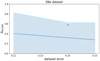 |
Fig. E.1. ΔΛCDM vs. the imposed error for the Pantheon data set (i.e., just supernovae). The dot stands for the experimental data, while the solid line and the shadowed region refer to the corresponding theoretical benchmarks, obtained as described in the text. |
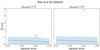 |
Fig. E.2. ΔΛCDM vs. the imposed error for the combined supernova + quasar sample at redshifts z < 2 (left panel) and z > 2 (right panel). The dots refer to the experimental data, while the solid lines and the shadowed regions stand for the corresponding theoretical benchmarks, obtained as described in the text. |
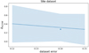 |
Fig. E.3. ΔΛCDM vs. the imposed error for the Pantheon data set (i.e., just supernovae). The reference mean and variance (represented as a shaded region) are shown in blue. The dot is obtained by processing the synthetic example generated via the CPL model. |
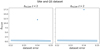 |
Fig. E.4. ΔΛCDM vs. the imposed error for the combined supernova + quasar sample at redshifts z < 2 (left panel) and z > 2 (right panel). The reference mean and variance (represented as a shaded region) obtained with mock ΛCDM samples are shown in blue. The dots are obtained by processing the synthetic example generated via the CPL model. |
In Fig. E.2 we analyze the full data set (Pantheon + quasars). The regression was hence carried out by considering data spanning the whole range in z. After the fitting was performed, data were split into two different regions: at low (z ≤ 2) or high (z ≥ 2) redshifts. The dots refer to the experimental data set and are set to the estimated error (0.14). The portion of the data set at low redshifts (mostly populated by supernovae) is compatible with a ΛCDM model with Ωm = 0.3, within statistical errors. The agreement is even more pronounced when the regression is carried out solely accounting for supernovae (see Fig. E.1). Conversely, for z > 2, the point computed after available experiments, notably experiments involving quasars, is at a distance of about 5σ from the expected value of the indicator ΔΛCDM. Hence, accounting for quasars enables us to conclude that the ΛCDM model is indeed extremely unlikely.
In Figs. E.3 and E.4 we repeat the analysis by employing a data set generated from a CPL model, with an error compatible with that estimated from experiments (equivalent to data sets D and F). The results indicate that accounting for data at high redshifts is mandatory for resolving the degeneracy between distinct generative models.
As a final point we elaborate on the reason why different models appear indistinguishable at low z. Function INN is the argument of a functional that goes from the space of function I to the space of the predictions. The way these two spaces communicate (or rather how function I reverberates on every ypred) is a nontrivial function of the hyperparameters (e.g., Ωm and the integration steps) and the domain explored. To clarify this point, we plot the functional derivative  (evaluated at the ΛCDM model) against Ωm and z. Via a visual inspection of Fig. E.5, the relevant impact of a low z and a large Ωm is evident. The functional derivative is hence very small for the portion of the data set that is populated by the vast majority of supernova entries. This implies that different models (in terms of the associated I(z) ) can yield very similar predictions. It is hence difficult to draw conclusions about the validity of different models if one solely deals with data at low redshifts.
All Tables
All Figures
|
Fig. 1. I(z) Results of the NN analysis of the Hubble diagram of simulated data. Top left: data set C, with the same redshift distribution and dispersion as the Pantheon supernova sample. Bottom left: data set E, where combined Pantheon and quasars are considered. In this case, the NN is able to identify the model assumed for data generation (the green shadowed region contains the exact profile for INN(z), depicted with a dashed line). The corresponding loss function is also shown and displays a minimum at the correct value of ΩM. Top right: Pantheon-like sample assumed for a CPL generative model (data set E). The NN is unable to distinguish between different scenarios (ΛCDM vs. CPL). Bottom right: CPL model with the inclusion of quasars. The degeneracy is resolved, and the NN can correctly identify the underlying model (see the dashed line). The loss shows a minimum for the correct value of ΩM, which yields the green shadowed solution for INN(z) vs. z. |
| In the text | |
|
Fig. 2. Results of the NN analysis of the Hubble diagram of supernovae (blue points in the middle panel) and quasars (red points). Top panel: estimated values of I(z) for different values of ΩM. Central panel: Hubble diagram with the reconstructed best-fit function obtained from the NN analysis. Bottom panel: Loss values for different values of ΩM. Notice that the solution visually closer (accounting for statistical errors) to the reference ΛCDM profile yields a significantly larger loss value and, as such, should be disregarded. The Loss is indeed nearly flat for ΩM < 0.3. |
| In the text | |
|
Fig. 3. Best-fit I(z) from our NN regression (as in the upper panel of Fig. 2) in logarithmic scale, compared with the function IMATTER(z) obtained by assuming w(z)≡0 in Eq. (3). The redshift intervals where the derivative of I(z) is higher than that of IMATTER(z) represent “matter-like” contributions, while intervals with a lower derivative refer to energy-like contributions. |
| In the text | |
|
Fig. D.1. Simulations with a "perfect" sample (data set A): results of the NN analysis of a simulated sample of 4,000 objects with a log-flat redshift distribution and a negligible dispersion with respect to a flat ΛCDM model with ΩM = 0.3. Top panel: Estimated values of I(z) for different values of ΩM (Eq. 3; the "correct" value for the simulated data is I(z)≡0). Central panel: Hubble diagram with the reconstructed best-fit function obtained from the NN analysis. Bottom panel: Loss values for different values of ΩM. The minimum is at ΩM = 0.3, i.e., the "true" value. The corresponding I(z) is consistent with zero at all redshifts. These results demonstrate that the NN analysis is able to recover the correct model and the "true"value of ΩM. |
| In the text | |
|
Fig. D.2. Results for data set B. The governing model is a CPL with w0 = −1.5, wa = 0.5. |
| In the text | |
|
Fig. E.1. ΔΛCDM vs. the imposed error for the Pantheon data set (i.e., just supernovae). The dot stands for the experimental data, while the solid line and the shadowed region refer to the corresponding theoretical benchmarks, obtained as described in the text. |
| In the text | |
|
Fig. E.2. ΔΛCDM vs. the imposed error for the combined supernova + quasar sample at redshifts z < 2 (left panel) and z > 2 (right panel). The dots refer to the experimental data, while the solid lines and the shadowed regions stand for the corresponding theoretical benchmarks, obtained as described in the text. |
| In the text | |
|
Fig. E.3. ΔΛCDM vs. the imposed error for the Pantheon data set (i.e., just supernovae). The reference mean and variance (represented as a shaded region) are shown in blue. The dot is obtained by processing the synthetic example generated via the CPL model. |
| In the text | |
|
Fig. E.4. ΔΛCDM vs. the imposed error for the combined supernova + quasar sample at redshifts z < 2 (left panel) and z > 2 (right panel). The reference mean and variance (represented as a shaded region) obtained with mock ΛCDM samples are shown in blue. The dots are obtained by processing the synthetic example generated via the CPL model. |
| In the text | |
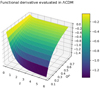 |
Fig. E.5. Plot of the functional derivative computed with Eq. (E.2) and varying Ωm and z. |
| In the text | |
Current usage metrics show cumulative count of Article Views (full-text article views including HTML views, PDF and ePub downloads, according to the available data) and Abstracts Views on Vision4Press platform.
Data correspond to usage on the plateform after 2015. The current usage metrics is available 48-96 hours after online publication and is updated daily on week days.
Initial download of the metrics may take a while.