| Issue |
A&A
Volume 678, October 2023
|
|
|---|---|---|
| Article Number | A171 | |
| Number of page(s) | 31 | |
| Section | Interstellar and circumstellar matter | |
| DOI | https://doi.org/10.1051/0004-6361/202244520 | |
| Published online | 20 October 2023 | |
The impact of H II regions on giant molecular cloud properties in nearby galaxies sampled by PHANGS ALMA and MUSE
1
Institut de Recherche en Astrophysique et Planétologie (IRAP), Université Paul Sabatier,
14 Av. Edouard Belin,
31400
Toulouse cedex 4,
France
2
IRAM,
300 rue de la Piscine,
38406
Saint-Martin-d’Hères,
France
e-mail: This email address is being protected from spambots. You need JavaScript enabled to view it.
3
LERMA, Observatoire de Paris, PSL Research University, CNRS, Sorbonne Universités,
75014
Paris,
France
4
Institut Laue-Langevin,
71 avenue des Martyrs – CS 20156,
38042
Grenoble cedex 9,
France
5
Department of Physics, University of Connecticut,
Storrs, CT,
06269,
USA
6
Department of Astronomy & Astrophysics, University of Chicago,
5640 South Ellis Avenue,
Chicago, IL
60637,
USA
7
Astronomisches Rechen-Institut, Zentrum für Astronomie der Universität Heidelberg,
Mönchhofstraße 12-14,
69120
Heidelberg,
Germany
8
Universität Heidelberg, Zentrum für Astronomie, Institut für Theoretische Astrophysik,
Albert-Ueberle-Str 2,
69120
Heidelberg,
Germany
9
International Centre for Radio Astronomy Research, University of Western Australia,
7 Fairway,
Crawley WA,
6009,
Australia
10
Universität Heidelberg, Interdisziplinäres Zentrum für Wissenschaftliches Rechnen,
Im Neuenheimer Feld 205,
69120
Heidelberg,
Germany
11
Sterrenkundig Observatorium, Universiteit Gent,
Krijgslaan 281 S9,
9000
Gent,
Belgium
12
Argelander-Institut für Astronomie, Universität Bonn,
Auf dem Hügel 71,
53121
Bonn,
Germany
13
The Observatories of the Carnegie Institution for Science,
813 Santa Barbara Street,
Pasadena, CA
91101,
USA
14
INAF – Osservatorio Astrofísico di Arcetri,
Largo E. Fermi 5,
50157
Firenze,
Italy
15
Departamento de Astronomía, Universidad de Chile,
Casilla 36-D,
Santiago,
Chile
16
Department of Physics & Astronomy, University of Wyoming,
Laramie, WY
82071,
USA
17
European Southern Observatory,
Karl-Schwarzschild Straße 2,
85748
Garching bei München,
Germany
18
Univ. Lyon., Univ. Lyon 1, ENS de Lyon, CNRS, Centre de Recherche Astrophysique de Lyon UMR5574,
69230
Saint-Genis-Laval,
France
19
Research School of Astronomy and Astrophysics, Australian National University,
Canberra, ACT
2611,
Australia
20
ARC Centre of Excellence for All Sky Astrophysics in 3 Dimensions (ASTRO 3D),
Australia
21
Center for Astrophysics | Harvard & Smithsonian,
60 Garden Street,
Cambridge, MA
02138,
USA
22
Department of Astronomy, The Ohio State University,
140 West 18th Avenue,
Columbus, OH
43210,
USA
23
Max-Planck-Institut für extraterrestrische Physik,
Giessenbachstraße 1,
85748
Garching,
Germany
24
School of Mathematics and Physics, University of Queensland,
St Lucia
4067,
Australia
25
Department of Physics, Tamkang University,
No. 151, Yingzhuan Road, Tamsui District,
New Taipei City
251301,
Taiwan
26
Observatorio Astronómico Nacional (IGN),
C/Alfonso XII, 3,
28014
Madrid,
Spain
27
Department of Physics, University of Alberta,
Edmonton, AB
T6G 2E1,
Canada
28
Max-Planck-Institut für Astronomie,
Königstuhl 17,
69117
Heidelberg,
Germany
29
Department of Physics and Astronomy, McMaster University,
1280 Main Street West,
Hamilton, ON
L8S 4M1,
Canada
30
Canadian Institute for Theoretical Astrophysics (CITA), University of Toronto,
60 St George Street,
Toronto, ON
M5S 3H8,
Canada
31
Sub-department of Astrophysics, Department of Physics, University of Oxford,
Keble Road,
Oxford
OX1 3RH,
UK
Received:
15
July
2022
Accepted:
3
May
2023
Abstract
Context. The final stages of molecular cloud evolution involve cloud disruption due to feedback by massive stars, with recent literature suggesting the importance of early (i.e., pre-supernova) feedback mechanisms.
Aims. We aim to determine whether feedback from massive stars in H II regions has a measurable impact on the physical properties of molecular clouds at a characteristic scale of ~ 100 pc, and whether the imprint of feedback on the molecular gas depends on the local galactic environment.
Methods. We identified giant molecular clouds (GMCs) associated with H II regions for a sample of 19 nearby galaxies from catalogs of GMCs and H II regions released by the PHANGS-ALMA and PHANGS-MUSE surveys, using the overlap of the CO and Hα emission as the key criterion for physical association. We compared the distributions of GMC and H II region properties for paired and non-paired objects. We investigated correlations between GMC and H II region properties among galaxies and across different galactic environments to determine whether GMCs that are associated with H II regions have significantly distinct physical properties compared to the parent GMC population.
Results. We identify trends between the Hα luminosity of an H II region and the CO peak brightness and molecular mass of GMCs that we tentatively attribute to a direct physical connection between the matched objects, and which arise independently of the underlying environmental variations of GMC and H II region properties within galaxies. The study of the full sample nevertheless hides a large galaxy-to-galaxy variability.
Conclusions. At the ~100 pc scales accessed by the PHANGS-ALMA and PHANGS-MUSE data, pre-supernova feedback mechanisms in H II regions have a subtle but measurable impact on the properties of the surrounding molecular gas, as inferred from CO observations.
Key words: HII regions / ISM: clouds / evolution / galaxies: ISM
© The Authors 2023
 Open Access article, published by EDP Sciences, under the terms of the Creative Commons Attribution License (https://creativecommons.org/licenses/by/4.0), which permits unrestricted use, distribution, and reproduction in any medium, provided the original work is properly cited.
This article is published in open access under the Subscribe to Open model. This email address is being protected from spambots. You need JavaScript enabled to view it. to support open access publication.
1 Introduction
Stellar feedback is a key process in galaxy evolution. Simulated galaxies without feedback cannot reproduce the observed properties of galaxies: they cool too rapidly, exhausting their gas supply through the rapid transformation of gas into stars (e.g., Schaye et al. 2015). On cloud scales, stellar feedback is often invoked to explain the low observed efficiency of star formation in giant molecular clouds (GMCs), which convert only ~1% of their mass into stars per cloud free-fall time (Krumholz 2014; Fujimoto et al. 2016; Utomo et al. 2018; Grudić et al. 2019; Kim et al. 2021b). On larger scales, stellar feedback contributes to driving galactic winds and outflows (Hopkins et al. 2012; Bolatto et al. 2013). Stellar feedback processes include protostellar jets and outflows, stellar winds, direct radiation from stars that can ionize the gas, reprocessed radiation from interstellar dust, and supernovae (Krumholz et al. 2019; Chevance et al. 2023). While there is a consensus about the overall importance of stellar feedback, much work remains to be done to quantify the timescales, efficiencies, and relative importance of the various forms of feedback across the diversity of galactic environments that host star formation.
The impact of stellar feedback on the surrounding molecular gas has been investigated on approximately parsec scales in individual Galactic star-forming regions (Pabst et al. 2019; Watkins et al. 2019; Barnes et al. 2020; Großschedl et al. 2021; Luisi et al. 2021; Olivier et al. 2021) and in Local Group targets (Lopez et al. 2011, 2014; McLeod et al. 2018, 2019, 2020, 2021). These studies underline the importance of pre-supernovae feedback. Further afield, studies of star formation and feedback in the nearby galaxy population have investigated the properties of H II regions and GMCs in their galactic context (Barnes et al. 2021; Rosolowsky et al. 2021), the efficiency of star formation within the molecular gas reservoir (Utomo et al. 2018), the relative spatial configuration and intensity of the CO and Hα emission (Schinnerer et al. 2019; Chevance et al. 2020; Pan et al. 2022), and the inferred timescales for various phases of the star formation process.
One outstanding question is whether feedback from star formation significantly modifies the properties of their natal clouds, not only at the immediate working surface, but also on the ~50–100 pc scales on which global cloud properties are typically measured. In this paper we study the impact of the H II regions on the surrounding molecular gas by exploring the properties of molecular clouds that are spatially coincident with H II regions identified in 19 nearby galaxies. This study leverages recent data from the PHANGS-ALMA and PHANGS-Multi Unit Spectroscopic Explorer (MUSE) surveys1 (Leroy et al. 2021a,b; Emsellem et al. 2022), which have characterized several tens of thousands of GMCs in 88 galaxies (Rosolowsky et al. 2021) and a similar number of H II regions in a subset of 19 galaxies (Santoro et al. 2022). Our study is complementary to the detailed, parsec-scale studies of individual star-forming regions that can obtain estimates of individual feedback terms (Barnes et al. 2021, 2022) since it provides an overview of how stellar feedback impacts the molecular gas reservoir across a wide range of galactic environments and interstellar conditions. By analyzing the properties of neighboring clouds and H II regions, it likewise offers a complementary view to previous pixel-based analyses that have robustly characterized the statistical relationship between the molecular gas reservoir and star formation activity (most notably to obtain evolutionary timescales of the star formation process; e.g., Chevance et al. 2020, 2022; Kim et al. 2022) but have so far been less focused on the physical properties of the star-forming gas.
Section 2 summarizes the properties of the PHANGS-ALMA and PHANGS-MUSE data, and of the GMC and H II region catalogs derived from those data. Section 3 presents the method that we use to match GMCs with H II regions. Section 4 compares the properties of matched GMC–H II regions to the general population of GMCs and H II regions in our sample galaxies. In Sect. 5, we investigate the correlations between GMC properties and H II region luminosity for the matched GMC–H II regions. In Sect. 6, we investigate whether the effects of local radiative feedback can be robustly distinguished from covariations of GMC and H II region properties within different galactic environments. Section 8 discusses the results, and Sect. 9 summarizes our findings. Appendices A–E present supplemental figures and tests of our methodology that complement the main content of the article. For instance, Appendix D examines the correlations between GMC properties and H II region luminosity in individual galaxies.
2 Data and catalogs
In this paper we compare the GMC and H II region populations of 19 galaxies in the PHANGS sample with both ALMA CO(2–1) (Leroy et al. 2021a,b) and MUSE Hα imaging (Emsellem et al. 2022). Table 1 summarizes the properties of our 19 target galaxies, which are adopted from the PHANGS Sample Table v1.6 (Leroy et al. 2021b). For the analysis in Sect. 6, we use estimates for the local stellar surface density presented by Sun et al. (2022). In this section we summarize the key properties of the PHANGS-ALMA and PHANGS-MUSE data and of the GMCs and H II-region catalogs derived from those data.
2.1 PHANGS-ALMA CO (2–1) data
We analyze GMCs that are identified in the PHANGS-ALMA survey of nearby galaxies (Leroy et al. 2021a,b). The GMC catalogs that we use are derived from the combined 12m+7m+TP PHANGS-ALMA CO(2–1) data cubes, which have a spectral resolution of 2.5 km s−1 and a typical angular resolution of ~1″ to 1.5″, corresponding to linear resolutions between ~30 and ~180 pc at the distance of our target galaxies. These combined cubes are sensitive to emission from all spatial scales. The PHANGS-ALMA observations were designed to target the region of active star formation in each galaxy, with a field of view that typically extends to R ~ 0.3R25. The mean 1σ sensitivity of the cubes is ~0.2 K per spectral channel. An overview of the PHANGS-ALMA survey science goals, observing strategy, and data products is presented in Leroy et al. (2021b). A detailed description of the PHANGS-ALMA data processing, including calibration, imaging and combination steps, is presented in Leroy et al. (2021a). The PHANGS-ALMA CO(2–1) data cubes are available from the PHANGS team website2, the ALMA archive3 and the Canadian Astronomy Data Center (CADC)4.
2.2 PHANGS-ALMA GMC catalogs
We used the public GMC catalogs released by PHANGS-ALMA on the PHANGS team website. These catalogs were generated using PYCPROPS5, which is a PYTHON implementation of the CPROPS algorithm originally presented in Rosolowsky & Leroy (2006). A detailed description of the PYCPROPS methodology, including its application to a subsample of ten PHANGS-ALMA CO(2–1) data cubes, is presented in Rosolowsky et al. (2021). The full set of GMC catalogs for 88 galaxies in the PHANGS-ALMA survey is presented in a companion paper by Hughes et al (in prep.). We refer the reader to those papers for a complete description of the PHANGS-ALMA GMC catalogs, but briefly summarize here the catalog generation process and the derivation of the key quantities that we use in our analysis.
Catalog generation by PYCPROPS proceeds in two main stages. First, significant emission in the data cube is identified. The emission is then segmented into distinct structures (“clouds” for simplicity) by identifying significant local maxima and uniquely assigning all the emission to each of these maxima. The criteria used to identify and segment the significant emission in the PHANGS-ALMA CO(2–1) data cubes are explained in detail by Rosolowsky et al. (2021). In short, the decomposition for the PHANGS-ALMA GMC catalogs proceeds by searching for regions larger than the telescope beam with intensities > 2σ that are contiguous in position and velocity with > 4σ peaks. Compactness is strongly preferred, such that local maxima are rarely merged into larger structures.
In a second step, the emission associated with each cloud is characterized, and physical properties of the cloud are determined. PYCPROPS uses moments of the emission to estimate cloud properties. The moment-based quantities are corrected for the effects of sensitivity and the finite resolution of the data before translating them into estimates of physical quantities. In this paper we investigate correlations involving the following GMC properties.
The CO peak temperature, Tpeak. This is the CO brightness temperature, measured at the brightest voxel within the cloud boundary.
Cloud molecular mass, Mco. We use the CO-based GMC mass estimate, which is obtained by multiplying the cloud luminosity Leo by a CO-to-H2 conversion factor, αCO. The cloud luminosity is the sum of the intensity within the cloud boundary, and is related to the mass via MCO = αCOLCO. The PHANGS-ALMA GMC catalogs implement the αCO calibration of Sun et al. (2020), with an adopted CO(2–1) to CO(1–0) line ratio R21 = 0.65. The αCO adopted for each cloud depends only on the local metallicity, which is estimated according to the global mass-metallicity scaling relation of Sánchez et al. (2019) and the universal metallicity gradient of Sánchez et al. (2014). We refer the reader to Sun et al. (2020) for a more complete discussion. Due to the restricted range of metallicities of our sample galaxies, LCO and MCO are effectively interchangeable for our analysis in this paper.
Cloud surface density, Σmol. We estimate the typical molecular gas surface density within the cloud as Σmol = MCO/(2πR2).
Cloud radius at FWHM, R. The cloud size is estimated from the intensity-weighted second moments over the two spatial axes of the cube (i.e., the spatial variances  and
and  ), and an intensity-weighted covariance term σxy. These measurements are used to determine the major and minor axes of the emission distribution and the cloud’s position angle. The major and minor axis measurements are corrected for the finite sensitivity and angular resolution of the data, σmaj,corr and σmin,corr. The cloud radius is then calculated as
  , with
  .
.
The characteristic turbulent linewidth at a fiducial scale of 1 pc, σ0. To estimate σ0, we assume that the turbulent structure function within all clouds has an index of 0.5 (e.g., Heyer & Brunt 2004). It is related to the observed cloud-scale velocity dispersion συ according to  . Here, συ is the square root of the intensity-weighted variance of the emission along the spectral axis within the cloud boundary, and R3D is an estimate for the three-dimensional mean radius of the cloud. R3D differs from the projected full width at half maximum (FWHM) size, R. In practice,
 (1)
(1)
where H = 100 pc is the assumed scale-height of the molecular gas in a galactic disk (Malhotra 1994).
Virial parameter of the whole cloud, αvir. This provides an estimate of the relative strength of the gravitational binding energy versus the kinetic energy of a molecular cloud. The PHANGS-GMC catalogs adopt  .
.
Free-fall collapse time, τff, which is derived from a combination of the above quantities as
 (2)
(2)
The factor of 4 in the denominator arises from the adopted two-dimensional Gaussian cloud model, which measures the density assuming half the mass is contained within the FWHM cloud size.
Properties of our galaxy sample.
2.3 PHANGS-MUSE data description
We used observations from the Multi Unit Spectroscopic Explorer (MUSE) at the Very Large Telescope (VLT; Bacon et al. 2010), which is ideally suited for surveying nearby galaxies given its wide ~ 1 arcmin field of view and broad wavelength coverage (4800–9300 Å) at moderate (R ~ 2000) spectral resolution. The PHANGS-MUSE survey (PI: Schinnerer; Emsellem et al. 2022) provides optical integral field unit maps across the central star-forming disks of 19 nearby (D < 19 Mpc, 1″ <100 pc) spiral galaxies with low to moderate inclination (<60°). The region surveyed in each galaxy is matched to the PHANGS-ALMA coverage, requiring several MUSE pointings per galaxy.
The typical seeing during our observations was 0.8″ in the R band, which corresponds to a typical physical scale of ~70 pc for our galaxies. This is well matched to the PHANGS-ALMA observations, and is adequately sampled by the 0.2″ pixel size. To create a datacube corresponding to the full observed field of view for each galaxy, the data for individual pointings were first convolved such that the point spread function is uniform for each galaxy before combination. We fit all stellar continuum emission (spatially binned to a S/N > 35) simultaneously with the emission lines (where we fit each individual pixel) on the resulting combined cube. The resulting maps of the Hα line emission are then used to identify the individual H II regions that are used in this work. Full details of the data reduction and production of emission line maps for PHANGS-MUSE are presented in Emsellem et al. (2022).
2.4 PHANGS-MUSE H II region catalogs
To locate and characterize the H II regions, we used the nebular catalogs compiled by Santoro et al. (2022) and described fully in Groves et al. (2023). They were constructed by applying the HIIphot algorithm (Thilker et al. 2000) to the PHANGS-MUSE Hα line maps.
The key physical properties of the identified objects in the catalogs are derived using integrated spectra within the footprint of each region, assuming Gaussian line profiles and correcting for the instrumental dispersion along the spectral axis at location of the Hα line (~49 km s−1, Bacon et al. 2017). To select the H II regions from the nebular catalogs, we select regions that have properties consistent with photo-ionization by massive stars by applying the [O III]/Hβ versus [N II]/Hα (Kauffmann et al. 2003) and [O III]/Hβ versus [S II]/Hα (Kewley et al. 2001) demarcations, excluding any nebulae where any of these lines has a signal-to-noise ratio of less than 3. We further exclude nebulae that overlap with foreground stars or overlap with the edge of our fields.
In this paper we work primarily with the total Hα luminosity, L(Hα), and size of the H II regions. The H II region size is defined as the circularized radius equivalent to the pixel area found in each H II region footprint. The total Hα luminosity is obtained from the sum of the Hα within the H II region footprint. The L(Hα) measurements that we use are corrected for dust extinction: a global extinction correction for each galaxy is applied to account for foreground extinction in the Milky Way (Schlafly & Finkbeiner 2011), and an individual extinction correction for each H II region that accounts for the dust within the target galaxy is determined using the observed Balmer decrement (Hα/Hβ). The latter assumes a Milky Way extinction curve (O’Donnell 1994) with RV = 3.1. We refer the reader to Groves et al. (2023) for a more detailed explanation of the H II region property definitions and of the corrections that are applied for, for example, extinction and instrumental resolution. As described in the catalog paper, derived physical quantities including metallicity (Pilyugin & Grebel 2016), Hα linewidth, and ΣSFR, are briefly considered in our analysis, but not explored in depth.
3 A method for matching GMCs and H II regions
Our science goal is to determine whether H II regions influence the physical properties of GMCs. In this section we describe the method that we use to determine whether a GMC and H II region are physically associated. Specifically, we worked with catalogued measurements of the radial velocity of each GMC and H II region, and the pixel masks that are generated during the cataloging process to identify the boundaries and projected area of each region. The key criterion in our matching method is the spatial overlap between the projected areas of the GMCs and H II regions. We used the pixel masks of the GMC and H II regions to identify and measure regions of overlap. The H II region masks were re-projected using nearest-neighbor interpolation to match the astrometry and pixelization scheme of the GMC masks. We superposed the binary masks of each galaxy to identify pixels that are common to both GMCs and H II region masks. We constructed a list of the GMCs that are members of regions with common pixels and calculated the percentage of the projected area of each GMC that is also present within an H II region footprint. We considered an H II region to be paired with a GMC when it occupied more than a minimal overlap percentage (MOP) of the GMC’s projected area. We did not, however, consider the percentage of the H II region covered by the GMC. This makes our pairing method asymmetric. This is physically motivated in the sense that we searched for potential signatures of H II region feedback on GMC properties at a scale of ~100 pc. We thus prioritized the detection of pairs where the H II region covers a significant fraction of the GMC area. From our initial list of paired regions, we excluded candidate pairs where the difference between the radial velocity of the GMC and H II region was larger than 10 km s−1.
We found it necessary to refine our basic approach for the relatively common situation where a single GMC has pixels that overlap multiple H II regions (or vice versa). Of the total number of GMCs that share common pixels with H II regions, approximately half (47%) overlap with more than one H II region. For H II regions, the fraction is smaller (19%). We decided to allow each GMC to have more than one associated H II region, but required that H II regions be uniquely identified with a GMC, in practice assigning it to the GMC that is most covered by the H II region’s projected area. We discuss the rationale for this approach and compare it to other possible choices, for example using only exclusive GMCs-H II region pairs, in Appendix A.1.
Our matching approach is illustrated in Fig. 1. This figure shows the GMCs and H II regions within a spiral arm region of NGC 4254. The left panel illustrates the results for a MOP of 10%: here, GMC B is uniquely matched with H II region three, while GMC A is matched with both H II regions one and two. The right panel illustrates a MOP of 70%: here, only GMCs A and B remain, and now GMC A is uniquely matched with H II region two. For most of the analysis in this paper, we set MOP = 40%. Using a higher MOP value would allow us to pinpoint the GMCs where H II region feedback is likely to be the most pronounced, potentially making it easier to identify any signatures of feedback on the cloud properties. However, imposing higher MOP values would also reduce the number of identified pairs, making any conclusions less general. Our adopted MOP of 40% is thus a compromise, based on both physical and practical considerations. We present several tests of our method, and justify our choice for several user-defined parameters in Appendix A.3.
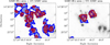 |
Fig. 1 Example results of the algorithm used to match GMCs (blue) and H II regions (red) for the same field of view. The background image is Hα line emission from a spiral arm segment in NGC 4254. The right and left panels show the matches obtained when the area of the GMC–H II region overlap is at least 10% and 70%, respectively, of the projected area of a GMC. Imposing a higher overlap percentage leads to fewer identifications of matched GMC–H II regions. |
Fraction of GMCs and H II regions that are identified as matched objects across our sample.
4 Properties of matched GMC-H II regions
We applied our GMC-H II region matching algorithm to the 19 galaxies that are common to the PHANGS-ALMA and PHANGS-MUSE surveys. In NGC 7496 and IC5332, our matching strategy failed to identity any matched GMC and H II region for some or all of the minimum overlap percentage thresholds that we used. For the rest of this paper, we therefore present results for the remaining 17 galaxies. In this section we compare the properties of matched GMC-H II regions with the typical properties of their parent distributions, as well as the impact of the adopted MOP on the detection statistics of matched regions and the property distribution shapes.
4.1 Detection of matched GMC–H II regions
Table 2 summarizes the overall results of our matching strategy, that is to say, the number of identified GMC-H II region pairs for MOP thresholds of 10, 40, and 70%, and the fraction of CO and Hα luminosity that the paired objects represent in each case. Not surprisingly, fewer matched GMC-H II regions are identified at higher MOP thresholds. Matched GMC-H II regions barely exceed 50% of their parent populations, even using a low MOP threshold of 10%. This is qualitatively consistent with previous studies that found a significant reservoir of quiescent CO-bright gas in galaxies and a relatively short timescale for its disruption by stellar feedback (e.g., Schinnerer et al. 2019; Chevance et al. 2022). Measured across our full sample, for a MOP threshold of 10%, the CO luminosity associated with GMCs in matched GMC-H II regions is 41%, which roughly corresponds to the number of clouds identified within these regions 39%. While fewer in number, the H II regions associated with matched GMC-H II regions make a more significant contribution to the total Hα luminosity (19.5% in number versus 48% in flux for a MOP threshold of 10%). Table B.1 presents the detection statistics and contribution to total CO and Hα luminosity of the matched GMC-H II regions for individual galaxies.
4.2 Properties of matched GMC–H II regions compared to their parent distributions
Figure 2 presents the empirical probability density functions (PDFs) of the size and luminosity of the H II regions and of several physical properties of GMCs (size, luminosity, peak temperature, velocity dispersion, surface density, characteristic turbulence linewidth, virial parameter, and free-fall time). The PDFs were computed using a kernel density estimation method. In each panel, the distribution of the parent population and of the matched objects using MOP criteria of 10, 40, and 70% are shown.
We conducted Kolmogorov-Smirnov tests6 and AndersonDarling tests7 to assess whether the differences in the distributions in Fig. 2 are statistically significant. If the influence of H II regions on GMCs is localized, then we expect that the trends in Fig. 2 will become more pronounced as we increase the adopted MOP. If the trends instead result from the covariation of GMC and H II region properties that are themselves due to larger scale effects (e.g., the colocation of clouds and H II regions in spiral arms), then we would expect the distributions to be less sensitive to the adopted minimum overlap percentage.
Figure 2d shows that matched GMCs are on average smaller than the parent population (mean radius of 45 pc versus 69 pc for a MOP threshold of 70%), whereas Fig. 2b shows that matched H II regions are on average bigger than the parent population. This difference is more pronounced for higher MOP thresholds and is mostly due to the asymmetry of our matching criteria. The effect is larger for the H II region sizes than for the GMC sizes. This is because our input GMC catalogs only contain resolved sources, while the H II region catalogs contain a large fraction (80%) of point sources.
Giant molecular clouds in the matched populations exhibit a larger fraction of clouds with high CO peak brightness than the overall GMC population, as shown in Fig. 2e. This cannot be due to our matching strategy, since GMCs generally show a marginally positive or no trend between their size and CO peak brightness. The luminosities of the GMCs and H II regions follow the size trends since these properties are correlated to first order. A population of luminous GMCs is still evident in the matched populations, however, even though there are relatively few large GMCs: In Fig. 2c the MOP = 70% (gold) population lies clearly above the parent GMC population (red) at high CO luminosity, even though there are more large GMCs in the parent population. These trends in size and brightness reinforce each other to yield a clear progression in the typical surface density and inferred free-fall time (Figs. 2g,i) of the matched GMCs, such that GMCs in the matched population identified with MOP = 70% have roughly twice the surface density of the average GMC in the parent population, while the inferred typical free-fall time (which varies inversely with the surface density) of the matched GMCs is correspondingly shorter.
The distributions of cloud properties that involve the GMC velocity dispersion are more difficult to distinguish. In Figs. 2f,j, the average velocity dispersion and virial parameter of the matched GMCs are slightly smaller than those of the parent population, which is to be expected from their smaller typical size and slightly higher brightness. If the variation in the velocity dispersion was due purely to the cloud’s smaller size and the Larson size-linewidth relation, then we would expect the distributions of the characteristic turbulent linewidth at a fiducial scale of 1 pc to be the same for the matched and parent GMC populations. For the higher MOP thresholds, we instead see in Fig. 2h a slight shift toward a larger average characteristic turbulent linewidth, and a larger fraction of clouds with higher characteristic turbulent linewidths, suggesting we may statistically detect a contribution to the cloud linewidth in the GMCs with matched H II regions above and beyond the effect of cloud size. Potentially, this could reflect a slight increase of the turbulence within GMCs that closely associated with H II regions. The difference is small however (a shift of < 0.1 km s−1 pc−0.5 in the mean value).
The results of the tests that we conducted to determine whether the observed differences in the distributions are statistically are listed in Tables C.1 and C.2. While the Anderson-Darling test is less sensitive to outliers compared to the Kolmogorov-Smirnov test, both tests give similar results. For a minimum overlap percentage of 40% or above, all the distributions of the matched GMCs properties are statistically different from their parent distributions. This is also true for the characteristic turbulent linewidth, which shows only a small variation in the distribution mean for different adopted values of the MOP.
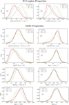 |
Fig. 2 PDFs of key physical properties of H II regions and of GMCs. Top, from left to right: Extinction-corrected Hα luminosity and size. Bottom, from top left to bottom right: CO luminosity, size, peak temperature, velocity dispersion, surface density, characteristic turbulent linewidth, free-fall time, and virial parameter. The distribution for the full GMC (H II region) population is shown in red, while the matched GMCs–H II regions adopting a MOP of 10, 40, and 70% are shown in blue, green, and gold, respectively. |
4.3 Intermediate summary
Below we summarize the results obtained in the paper thus far.
First, matched GMC-H II regions represent a non-negligible fraction of the overall GMC population in our sample galaxies. For a 10% minimum overlap percentage, 40% of the GMCs and one fifth of the H II regions are matched, and these matched pairs represent about 50% of the total CO and Hα luminosity that arises from the catalogued objects.
Second, all observed trends in the GMC property distributions are significant according to standard statistical tests.
Third, matched GMCs have a smaller size and higher typical CO peak temperature than a GMC from the overall population. The relative small size of the matched GMCs likely derives from the asymmetry of our adopted matching strategy.
Fourth, the observed distributions suggest that the GMCs matched with H II regions are denser than a typical GMC. The larger typical surface density is at least partly due to their higher intrinsic brightness at the pixel-level, as reflected in their higher typical peak CO brightness values.
Fifth, the virial parameter and free-fall time of matched GMCs have lower average values than the overall GMC population, which follows from the observed trends of their luminosity, size and velocity dispersion.
Finally, the characteristic turbulent linewidth of matched GMCs is slightly higher than for a typical GMC when a high (≥40%) MOP threshold is used.
For the rest of the paper, we focus on the mass, the peak brightness, the characteristic turbulent linewidth, and the molecular gas surface density of the GMCs. The last three are intensive cloud properties that are often invoked by theories to explain the star formation rate and feedback, and do not scale directly with the GMC size by construction.
5 Correlations between matched GMC properties and the Hα luminosity of the H II regions
In this section we investigate whether there are significant correlations between the properties of the matched GMCs and H II regions for our maximum MOP threshold (70%). We then investigate how the adopted MOP threshold influences the observed correlations between GMC and H II region properties, focusing on the Hα luminosity of the H II region as our primary independent variable, and describe two simple randomization tests that we used to determine whether the observed correlations could arise by chance. We characterize any observed correlations using a simple power-law fit and a goodness-of-fit statistic, which we present immediately below.
5.1 Characterizing a power-law fit
We characterized correlations by computing an ordinary least square power-law fit to the observed trends and the associated ±3σ levels from the fitted line. To assess the quality of the correlation, we computed the R2 coefficient, defined as
 (3)
(3)
where Yi represents the logarithm of the studied property for GMC i, 〈Y〉 is the mean of the logarithm of this property over the studied sample, and Fi represents the values predicted by our fit. The numerator is proportional to the variance of the logarithm of the studied GMC property, while the denominator is proportional to the variance of the logarithm of the property about the power-law fit of Hα luminosity of the H II region. A R2 value of 1 indicates that the correlation is exactly linear in log-log space. A R2 value of 0 indicates that the predicted properties Y are independent of the value of the X axis variable. In other words, the higher the R2 value, the better the GMC property is predicted by a power-law model from the Hα luminosity of the H II region.
We also computed confidence intervals on the R2 coefficients through a standard bootstrap approach. We refit a power law using data samples that were constructed by selecting N pairs from the original data with replacement, where N is the number of original pairs: on average, 36% of the pairs are different, implying that pairs are typically duplicated ~2 to 3 times. We repeated this operation 10 000 times, each time computing the R2 coefficient between the two quantities of interest. We then computed the 95% confidence interval associated with the distribution obtained from these 10000 trials.
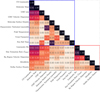 |
Fig. 3 Correlation matrix of the different GMC and H II region properties investigated. The top-left blue square shows the correlations between GMC properties considering the entire sample. The bottom-right red square shows the correlations between the properties of H II regions considering the entire sample. The bottom-left black rectangle shows the strengths of the correlations between matched GMC and H II regions for a MOP of 70%. |
5.2 Correlations between GMC and H II region properties
We first explore the correlations between the properties of matched GMC and H II regions. We compute the R2 coefficient between 1) GMC properties, 2) H II region properties, and 3) properties of GMCs and H II regions for matched pairs. Figure 3 presents the correlation matrices, which are sorted to display the strongest correlations in the top left corner of each matrix as far as possible. It shows that the virial parameter and free-fall time of GMCs are essentially uncorrelated with any of the H II region properties. In contrast, all other properties of the matched GMCs exhibit some degree of correlation with the properties of their associated H II regions. The Hα luminosity and star formation rate are highly correlated with the GMC luminosity and mass. Moderate correlations with these H II region properties are observed for the GMC size and velocity dispersion, with weaker correlations obtained for the GMC surface density, characteristics turbulent linewidth and CO peak temperature. The H II region velocity dispersion, metallicity, and stellar surface density exhibit correlations with the CO luminosity, molecular mass, size and velocity dispersion of the associated GMCs, but are mostly uncorrelated with the molecular surface density, characteristic turbulent width and CO peak temperature.
The CO luminosity and mass are tightly correlated, justifying that we use them interchangeably in the following. The GMC size and velocity dispersion are also well correlated with the molecular mass. These correlations reflect the well-known Larson scaling relations (Larson 1981). The characteristic turbulent linewidth shows a strong positive correlation with the velocity dispersion. As expected from their definitions, the free-fall time follows the molecular gas surface density.
The Hα luminosity is correlated with all the other H II region properties that we consider, albeit only weakly with the metallicity and local stellar surface density. Due to the additional strong covariance between the Hα luminosity and the size, star formation rate and velocity dispersion of the H II regions that we observe in Fig. 3, we restrict our comparison to studying GMC properties as a function of the H II region Hα luminosity for the remainder of the paper.
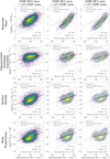 |
Fig. 4 Scatter plots of various GMC properties as a function of the Hα luminosity for three different MOPs of the H II–GMC pairs: 10% for the left column, 40% for the middle one, and 70% for the right one. The GMC properties are, from top to bottom: the molecular mass, the characteristic turbulent linewidth, the surface density, and the peak temperature. The solid black lines show a power-law fit and its uncertainty for each scatter plot. The dashed lines show the ±3σ levels from the fitted line. The solid red line represents the linear regressions obtained in the leftmost column, for comparison. The fitted line properties are displayed at the bottom-right corner of each panel. |
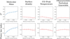 |
Fig. 5 R2 (top) and power-law index (bottom) of the fits of various GMC properties (as a function of the Hα luminosity of the matched H II region) against the MOP. The fitted GMC properties are, from left to right: the molecular mass, the peak temperature, the surface density, and the characteristic turbulent linewidth. Blue (respectively red) lines show an increase (respectively decrease) of the R2 coefficient with the MOP. The uncertainty intervals are computed using a standard bootstrap method. |
5.3 Evolution with the minimum overlap percentage
Figure 4 presents scatter plots of the GMC properties as a function of the Hα luminosity for three different MOP used to identify the GMC-H II region pairs: 10, 40, and 70%. To help visualize how the correlation changes with the MOP that we adopt, the solid red lines indicate the power-law fit for a minimum overlap percentage of 10% in all panels.
The Hα luminosities of the catalogued H II regions in our sample cover about five orders of magnitude, while the properties of matched GMCs cover a smaller dynamic range: ~1.5 dex for peak temperature, ~2 dex for the characteristic turbulent linewidth, up to ~3 dex for the surface density and molecular mass. The plots illustrate the correlations indicated by the matrix in Fig. 3: a good correlation between the GMC mass and the Hα luminosity of its associated H II region at all MOP thresholds, but weaker and more scattered relationships for the intensive cloud properties, especially at high MOP values. For a MOP threshold of 40%, the R2 values range from 0.12 for the peak brightness to 0.55 for the GMC molecular mass, indicating that GMC properties do indeed show a positive correlation with the Hα luminosity of the H II region. The power-law indices that we obtain range from 0.20 for the GMC surface density to 0.58 for the molecular mass. The GMC peak brightness and characteristic turbulent linewidth show intermediate power-law indices of 0.12 and 0.14, respectively. There is, however, structure in the plots in Fig. 4 that is not completely captured by a simple power-law fit, and which is most evident for the correlations involving intensive GMCs properties when the GMC-H II-region pairs are identified using higher (≥40%) MOP thresholds. Some of this structure in the correlation may be due to galactic environment, as we discuss in Sect. 6.
In Fig. 5, we plot how the R2 coefficients and the power-law slope of the observed correlations depend on the adopted MOP. When increasing the minimum overlap percentage from 10 to 70%, we find that the correlation between GMC molecular mass and the Hα luminosity of the matched H II regions clearly exhibits a higher R2 coefficient and a steeper power-law slope. The correlation with the CO peak temperature on the other hand marginally weakens with increasing MOP. The correlation of the GMC surface density and the characteristic turbulent linewidth with Hα luminosity of the matched H II regions show no dependence (within the confidence interval) on the adopted MOP.
5.4 Randomization tests to check whether the observed correlations are genuine
We conducted two tests to investigate whether the observed correlations reflect a potential physical influence of the H II regions on the GMCs. First, we randomized the Hα luminosities of the H II regions in the PHANGS-MUSE catalog, holding their positions and sizes constant. The properties and positions of the GMCs were also left unchanged. We then computed the R2 coefficients for the same set of correlations described above. We performed this randomization test 10 000 times in order to gauge the typical range of R2 values that might arise randomly. We obtained R2 values of 0 to 0.04 for all the properties, all lower than the lowest R2 value (0.15) that we obtained for the actual correlations (see Fig. C.1).
To assess whether the observed correlations are an artifact of our matching strategy, we next randomized both the sizes and the Hα luminosities of the H II regions, regenerated the list of matched GMC–H II regions, and constructed the same set of correlations as described above. This yields typical R2 values of 0 to 0.003, much lower than 0.15 (see Fig. C.2). We note that completely randomizing the positions of the H II regions is unfeasible, since the projected area occupied by H II regions and GMCs represents only 11.2% and 10.6% of the observed field of view. Assigning random positions to the GMCs or H II regions would thus result in no GMC–H II region pairs being detected.
5.5 Intermediate summary
The results obtained in the above section are outlined below.
First, a positive correlation between GMC properties (mass, surface density, CO peak brightness temperature, and characteristic turbulent linewidth) and the Hα luminosity of the matched H II regions exists for a MOP of 10%. The relationship between GMC properties and Hα luminosity of the matched H II region can be represented by a power law to first order.
Second, the dependence of GMC properties on the Hα luminosity of the matched H II region varies as a function of the minimum overlap percentage in diverse ways. On one hand, the strength of the correlation between the Hα luminosity and the molecular mass significantly improves as we increase the MOP. The correlations with the GMC surface density and the characteristic turbulent linewidth remain unchanged, and the correlation with the CO peak brightness temperature weakens for higher MOP thresholds.
Finally, the observed correlations cannot be reproduced in tests that randomize the Hα luminosity and/or sizes of the H II regions before and after identifying the matched GMC-H II region pairs.
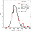 |
Fig. 6 PDFs of the stellar mass surface density within 500 pc of the matched GMC–H II regions. The global population in shown in red, and the matched population, with a MOP of 40%, in shown in black. The vertical dashed lines show the limits used to define the three stellar density environments in Sect. 6. |
6 Correlations within different galactic environments
Both the distributions of the GMC properties and their correlation with the H II region luminosity vary with the minimum overlap percentage that we use to identify a GMC–H II region pair. A possible explanation of these results is that GMC properties hosting H II regions are modified by local radiative feedback. Another possibility is that correlations between GMC and H II region properties arise from their covariation with the local galactic environment. It is thus important to consider whether the matched GMC–H II regions are preferentially located in certain galactic environments, and whether the galactic environment has an influence on the observed correlations. In this section we investigate the correlations as a function of the kiloparsec-scale environment surrounding the GMC–H II region pairs. Specifically, we focus on the stellar surface density. We explored a number of other large-scale properties of the galactic environment, such as the star formation rate surface density and molecular gas surface density, but found that they closely track the stellar surface density and give similar results as those presented below.
6.1 Method
To investigate whether there is a dependence on galactic environment, we sorted the GMC–H II region pairs into three equally populated bins of the local stellar surface density, which we measured within an aperture of radius 500 pc around each GMC–H II region pair using the stellar surface density maps of PHANGS galaxies presented by Sun et al. (2022). We used the GMC-H II region pairs identified using a MOP of 40 %, yielding 380 pairs per bin. For the sake of simplicity, we refer to the first bin as “low density environments” (0 ≤ log(Σ★/1 M⊙ pc−2) ≤ 2.0), the second bin as “average density environments” (2.0 ≤ log(Σ★) ≤ 2.9), and the last bin as “high density environments” (2.9 ≤ log(Σ★) ≤ 3.7).
Figure 6 shows the empirical PDF of the stellar surface density surrounding the GMC-H II region pairs. There is an observable difference between the distributions of the parent GMC population and of the GMCs that have an interface with an H II region (MOP of 40%). The number of GMCs that are matched with an H II region appears to decrease at the highest stellar surface densities. This effect is naturally explained if the timescale of significant interaction between GMCs and H II regions is shorter in regions of high stellar surface density.
Number and luminosity of GMCs and H II regions per galactic environment of the studied sample, for a MOP of 40%.
Continued
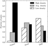 |
Fig. 7 Fraction of GMC-H II region pairs with low, medium, or high density environments in the galaxies’ center (nucleus and bar), arms, and disk (interarms and outer disk), for a MOP of 40%. |
6.2 Results
To illustrate how the stellar surface density bins relate to the commonly used dynamical environments, Fig. 7 presents the relative proportion of low, average and high stellar surface density environments that are present in the nuclear and bar regions of galaxies (henceforth referred to collectively as the center environment), in spiral arms, and in interarm regions and galaxy outer disks (henceforth referred to as the disk environment). Galaxy centers are almost exclusively composed of high stellar surface density environments. Low, average and high stellar surface density environments are present in roughly equal proportions within spiral arms. Galaxy disks are characterized by low stellar surface density environments. The detailed statistics of matched GMCs and H II regions per galactic environment are shown in Table 3.
Figure 8 shows the correlations between Hα luminosity and GMC properties for GMC-H II region pairs for each stellar surface density bin. The correlations between the Hα luminosity and the GMC properties are clearly different from one environment to the other: the correlations are stronger and steeper in the high stellar surface density environments, and less pronounced in the low stellar surface density environments.
The correlations involving the different GMC properties exhibit different trends with stellar surface density. A correlation between GMC mass and H II region luminosity persists across all bins, although it steepens with increasing stellar surface density. Correlations between the H II region luminosity and other intensive GMC properties, on the other hand, are weak to nonexistent in low stellar surface density environments, and only clearly emerge for log Σ★ > 2.
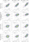 |
Fig. 8 Scatter plots of various GMC properties as a function of the Hα luminosity for different environmental stellar surface densities measured at a scale of 500 pc, in a similar fashion to Fig. 4. Each column represents a bin of environmental stellar surface density, as defined in Sect. 6. From left to right: low density, average density, and high density environments. The red line shows the global correlation from Sect. 5 with a MOP of 40%. |
6.3 Intermediate summary
Below is a summary of the results obtained in the above section.
First, the correlations between GMC properties and the Hα luminosity improve with increasing kiloparsec-scale stellar surface density. The correlations are the strongest in high stellar surface density environments, and either weaker (for the molecular mass) or nonexistent in lower stellar surface density environments.
Second, there is a strong correlation between the GMC mass and the H II region luminosity across the full range of kiloparsec-scale stellar surface densities in our sample (Fig. 8, top row). In contrast, the GMC surface density or peak temperature are uncorrelated with the H II region luminosity in low stellar surface density environments, while they become clearly correlated in high stellar surface density environments.
Third, the overall correlations between the CO peak temperature, molecular gas surface density and the H II region Hα luminosity seen in Fig. 4 are much weaker than the same correlations in the “dense” kiloparsec-scale environments seen in the right column of Fig. 8. This difference may partly be due to a dilution effect. GMC–H II region pairs in the low density environments accounts for a large fraction of the overall population of GMC–H II region pairs. The fact that they show a weaker correlation than average thus dilutes the correlation signature.
Finally, comparing Figs. 4 and 8 shows that the correlations of the intensive GMC properties with the H II region luminosity are much more sensitive to the kiloparsec-scale stellar density than to the MOP. This effect is weaker for the characteristic turbulent linewidth than for the peak temperature and surface density of GMCs. In contrast, the correlation of the GMC mass with the H II region luminosity is about as sensitive to the stellar density as it is to the MOP. This difference of behavior suggests that correlations involving the intensive properties may stem from covariations of GMC and H II regions properties with galactic-scale environment, while the correlation of the GMC mass with the stellar surface density is influenced by the local (i.e., cloud-scale) effects.
7 Correlations within individual galaxies
Our combined sample of H II regions and GMCs is drawn from 17 galaxies. Among their global properties, the inclination and distance of the host galaxies could have an impact on our matching procedure, and by extension on the correlations that we observe. In this section we investigate whether the correlations described in Sect. 5 exist within individual galaxies by considering galaxies separately, where observational effects, such as inclination, distance, and resolution, presumably do not play a role. For completeness, we also explored whether the correlations could be related to other galaxy properties, namely the total CO luminosity, total Hα luminosity, metallicity, stellar mass and distance from the star-forming main sequence. For this analysis, we use the list of matched GMC–H II region pairs identified using a MOP of 40%. We identify between 29 (for NGC 2835) and 227 (for NGC 1566) pairs in each galaxy in our sample, with a mean of 114 pairs per galaxy. This is sufficient to consider the correlations between GMC properties and H II region luminosity within individual galaxies, but prohibits exploring trends with stellar density within them.
We examined the correlations between GMC properties and the H II region luminosity using the same procedure as in Sect. 5, measuring the power-law slope and R2 statistic for each. A full list of our per-galaxy results is presented in Table D.1. For each of the GMC properties that we consider, we find significant variability among galaxies in terms of the slope and quality of a power-law fit. Consistent with the global trend in Sect. 5, the GMC mass tends to be well correlated with the Hα luminosity within individual galaxies, with moderate (R2 > 0.3) to strong (R2 > 0.5) correlations obtained for 13 galaxies. Few individual galaxies show a significant correlation between the H II region luminosity and the GMC surface density or characteristic turbulent linewidth, again consistent with the global trends. It is striking, however, that individual galaxies reveal a much stronger correlation between the CO peak brightness and H II region luminosity than can be discerned from the global trends, with R2 values that are comparable to those obtained for the correlations with GMC mass (i.e., R2 > 0.3 for 13 galaxies, and three galaxies with R2 > 0.5).
We explored whether there were any systematic trends between these correlation results and properties of the host galaxies by plotting the derived power-law slopes and R2 statistics against galaxy distance, inclination, stellar mass, total CO and Hα luminosity, mean log Σ★, offset from the star-forming main sequence, and number of pairs identified. These results are presented in Appendix D. We find no dependence of the strength and slope of the observed correlations on the inclination or distance to the galaxy, suggesting that the correlations are not driven by geometric effects (e.g., viewing angle) or resolution. In general, lower mass systems in our sample tend to exhibit poorer correlations between the GMC properties and the H II region luminosity. Since the typical stellar surface density in galaxy disks tends to scale with the galaxy total mass and luminosity, this result is consistent with the weaker correlations observed for low stellar surface density galactic environments that we described in Sect. 6.
8 Discussion
In this study we searched for evidence for a potential impact of H II regions on GMC properties as measured on spatial scales between 30 and 180 pc. We presented a method for matching H II regions to a GMC based on their relative overlap region.
We studied (1) the distributions of characteristic cloud properties (molecular mass, surface density, CO peak temperature, and characteristic turbulent linewidth) of GMCs that are associated with H II regions, and how these distributions vary as a function of the MOP that we adopt to identify matched objects, and (2) correlations between GMC properties and the Hα luminosity of their associated H II regions, again as a function of the MOP. To establish whether our results are consistent with the observed correlations having a local origin (i.e., a direct physical link between the cloud’s physical state and the H II region), we investigated whether the correlations vary with the kiloparsec-scale stellar surface density, and global properties of the host galaxy, including observational properties such as distance and inclination.
In this section we briefly summarize the trends that we observe and outline three potential physical scenarios that could explain them. To conclude, we summarize the lessons learnt during this exercise.
8.1 Two families of behaviors experienced by the properties of the GMC–H II region pairs with increasing overlap
Figure 9 presents the joint and marginalized PDFs of the GMC molecular mass and CO peak temperature and the Hα luminosity of its associated H II region for two minimum overlap percentage thresholds: 1% in red, and 70% in blue. A MOP threshold of 1% yields a good approximation for all the GMCs that are contiguous or overlapping with at least one H II region. We used a kernel method to compute all the PDFs. Figure 9 illustrates that increasing the MOP causes two distinct effects on the correlations between GMC properties and the Hα luminosity.
First, the CO peak temperature (and the other intensive properties) demonstrate one behavior when we vary the overlap criterion: as we impose a higher MOP increases, the median value of the GMC property also significantly increases. This behavior reduces the dynamic range of the x and y axis values, reducing the R2 value of the correlations.
Second, the GMC mass shows a different behavior: its correlation with the Hα luminosity strengthens and steepens. Additionally, the median shifts toward lower masses. The latter effect is mostly due to the asymmetry of the matching criterion.
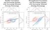 |
Fig. 9 Joint PDFs and their marginalized PDFs of the GMCs peak temperature (left) and molecular mass (right) with the matched H II region Hα luminosity for two MOPs: 1% in red and 70% in blue. The joint PDFs are shown as contour plots. The medians of the marginalized PDFs and the power laws fitted on the joint PDFs are overlaid as straight lines. |
8.2 Potential physical origin
The physical properties of GMCs follow Larson-type scaling relations, such that larger GMCs also tend to be more massive and more turbulent. Appendix E confirms that these relationships exist for the GMCs that we identify with H II regions using any MOP. However, these relationships fail to explain either why the CO peak temperature increases with the MOP or why the correlation of the GMC mass with the Hα luminosity strengthens when increasing the minimum overlap percentage. We consider three possible scenarios to explain these two observed behaviors.
The environmental scenario. The galactic environment induces covariation of GMCs and H II region properties without a direct causal connection between them.
The epigenetic scenario. Parent GMCs transmit some of the properties from their environment to their child H II regions.
The radiative feedback scenario. The child H II regions disrupt and alter the intrinsic properties of their parent molecular cloud.
The trends identified in our analysis are likely due to a combination of these scenarios. For instance, there could be a “background” covariation of matched GMCs and H II regions due to a common environment or to the heritage of some of the GMC properties to the associated H II regions, and local effects (e.g., stellar radiative feedback) could become the predominant driver of the GMC-H II region correlations only observed for highly overlapping pairs.
8.2.1 Environmental scenario
Section 6 first shows that the correlations between the GMC properties and the Hα luminosity are sensitive to the kiloparsec-scale stellar surface density, when considering all the matched GMC-H II region pairs. For instance, there is no correlation of the CO peak brightness and surface density with the Hα luminosity in low density kiloparsec-scale environments, but these correlations appear and improve systematically as a function of the kiloparsec-scale stellar density. This means that the kiloparsec-scale environment plays a role in setting the correlations of the GMCs properties with the luminosity of the matched H II regions.
However, Sects. 5 and 6 also show that the correlation between the Hα luminosity and the molecular mass is much more sensitive to the MOP than to the kiloparsec-scale environment. This argues in favor of a local origin of this behavior.
8.2.2 Epigenetic scenario
Section 5 shows a strong positive correlation between the H II region Hα luminosity and the molecular cloud mass. Moreover, this correlation increases in steepness and strength when increasing the MOP. Section 6 also shows that this correlation persists even in low density environments, where crowding is less of an issue. This suggests that this correlation is not driven by coincidental covariation of the GMC and H II region properties, but has a local origin. An evolutionary link offers a natural local origin: a high-mass GMC is needed to make a large and thus luminous H II region. In this scenario, GMC properties are partly regulated by their kiloparsec-scale environment. This information is transmitted to their child H II regions. This is similar to epigenetics (i.e., the study of how the environment can cause changes that affect the way genes work).
8.2.3 Stellar feedback scenario
The observed spatial de-correlation on small (<100pc) scales between molecular gas and young star forming regions (Schruba et al. 2010; Onodera et al. 2010; Grasha et al. 2018, 2019; Kreckel et al. 2018; Kruijssen et al. 2018, 2019; Schinnerer et al. 2019; Chevance et al. 2020) indicates that within the star formation cycle the clearing and dissolution of the natal molecular birth cloud must occur on relatively short timescales. Recent results indicate that pre-supernova feedback processes are essential contributors to this process (Barnes et al. 2021, 2022; McLeod et al. 2021; Olivier et al. 2021), with clearing times estimated to be only a few megayears (Kim et al. 2021a, 2022; Chevance et al. 2022). By isolating the subset of GMCs that overlaps with H II regions, it is possible that we are catching this process in the act. If this is the case, we expect to see some imprint on these feedback processes onto the parent GMC. Some tentative evidence for this was identified in the “Headlight cloud” in NGC 0628 (Herrera et al. 2020), where CO emission associated with this cloud was suggested to be overluminous due to heating by the associated H II region.
With our matched GMC and H II region sample, we identify a weak positive correlation between CO peak brightness and Hα luminosity (Fig. 4). This correlation is strongest within dense kiloparsec-scale environments, with R2 = 0.32. It clearly decreases with increasing overlap percentage (Fig. 5), and is essentially absent at minimum overlap percentages of 70%. Looking in low density kiloparsec-scale environments, where the cleanest matches are possible and there should be less contribution from neighboring or clustered star-forming regions, the correlation is absent (R2 = 0.00). Analysis of individual galaxies (Sect. 7), on the other hand, tends to confirm a trend between CO peak brightness and Hα luminosity, suggesting the scatter in Figs. 4 and 8 is at least partly due to galaxy-to-galaxy variation.
The CO peak temperature significantly shifts to higher values when the MOP increases (see Fig. 2 in Sect. 4). This shift effect happens even in low density environments, and thus probably has a local origin. Moreover, the origin of this local effect is completely independent from the strength of the correlation of the GMC mass with the Hα luminosity (see Appendix E). This independent effect could be explained by the fact that massive young stars naturally heat the Photon-Dominated Regions at the interface between H II regions and GMCs. The larger the MOP, the larger the interface and thus the more efficient heating. This effect would saturate the line peak brightness of the low-J CO lines and would enhance higher-J CO brightness.
We also look for a positive correlation between Hα luminosity and characteristic turbulent linewidth, and find a weak trend for any MOP. We identify a peak correlation at moderate 40% overlap percentage (R2 = 0.14). Nevertheless, the characteristic turbulent linewidth of matched GMCs shifts systematically toward higher values when we adopt a higher MOP (Sect. 4), the opposite behavior to συ that decreases in similar conditions. This could hint to a slight increase of the turbulent motion in GMCs by nearby H II regions.
8.3 Studying the impact of H II regions on GMCs: Lessons learned
Studying the impact of H II regions on GMCs in nearby galaxies on 30 to 180 pc scales is a difficult challenge for several reasons.
First, the PHANGS GMC and H II region catalogs present a large number of physical properties for each of these objects. This is a high-dimensional parameter space to be explored.
Second, some of the catalog properties are dependent by construction (e.g., the mass and size of GMCs). Even among physical properties that are in principle independent, there are well-established empirical correlations between GMC properties (e.g., Larson-type scaling relations) and between H II region properties.
Finally, the covariation among properties of GMCs and H II regions in different galactic environments can be larger than the impact of physical processes on cloud-scales and below that regulate the co-evolution of GMC and H II regions.
In summary, we are searching for subtle signatures in a high-dimensional space among properties that demonstrate preexisting correlations due to diverse physical origins. This implies we need to devise methods that maximize the probability of detecting a signature of H II region feedback on their natal GMC, without misinterpreting or biasing the results.
The timescale for disrupting GMCs via H II region feedback is relatively short compared to the cloud lifetime (Kim et al. 2021a; Chevance et al. 2022). We thus need to search for a transient state. This, as well as the considerations outlined above, tends to favor using a high MOP to pinpoint the GMCs where H II region feedback is most pronounced. The drawback of such a choice is that pairs with a large overlap percentage are rare, leading us to combine regions from different galaxies. This complicates the interpretation due to the different characteristic environments within galaxies of different types.
In this paper, we compromised by adopting a fiducial minimum overlap percentage of 40% and studying how the joint PDFs and correlations vary as a function of MOP thresholds between 10 and 70%. We also used an asymmetric matching criterion to focus on the H II regions that are most likely to impact GMC properties on the spatial scales that are accessible to PHANGS-ALMA (i.e., ~100 pc). Increasing the angular resolution of nearby galaxy imaging surveys would allow us to better locate the interfaces between matched GMCs and H II regions, while maintaining good statistics. A less time-consuming alternative would be to increase the angular resolution of the observations toward selected pairs to validate the scenarios envisaged here.
The covariation of GMC properties and H II regions properties is a further complication, since the signature of feedback can be mistakenly considered as scatter around preexisting correlations, while it actually is a hidden control variable. In other words, it is important to reveal how this (previously hidden) variable impacts preexisting correlations of GMC properties. Once again, much higher resolution observations of extragalactic high-mass star-forming regions would be useful to understand how feedback signatures might manifest themselves in lower resolution observations over a much larger sample.
9 Conclusions
In this paper we study the physical properties of GMCs associated with H II regions for 17 galaxies in the PHANGS-ALMA survey. Our primary goal was to determine whether GMC properties on cloud scales (here 30 to 180 pc) are modified by star formation feedback. We studied the distribution of four cloud properties (GMC mass, surface density, CO peak temperature, and characteristic turbulent linewidth) and the correlations between these properties with the Hα luminosity of the associated H II regions. The main conclusions of our study are as follows.
Matched GMC–H II regions represent a non-negligible fraction of the overall population of GMCs and H II regions in galaxies. Giant molecular clouds have a higher detection rate of matched regions than H II regions. When considering the detected flux rather than the number of detected objects, H II regions in matched pairs represent a larger fraction of their host galaxy’s Hα luminosity than the contribution of GMCs in matched pairs to the galaxy’s CO luminosity.
Matched GMCs tend to be denser than a typical GMC.
In all galaxies and environments, the GMC mass (as inferred from its CO luminosity) is well correlated with the Hα luminosity of its associated H II region. The GMC surface density, CO peak temperature, and characteristic turbulent linewidth exhibit weaker correlations with the Hα luminosity.
The galactic environment has an impact on the observed correlation between GMC mass and the Hα luminosity. The correlation is generally stronger and steeper in the dense kiloparsec-scale environments (typified by the centers and bars of galaxies), and weaker in the low density kiloparsec-scale environments (e.g., outer disks and interarms).
The correlations observed using the combined sample of matched GMC-H II regions from 17 galaxies obscures some galaxy-to-galaxy variability. In particular, individual galaxies often exhibit significant correlations between the molecular mass, the CO peak temperature, and the Hα luminosity. The correlation with GMC mass persists when the combined sample is considered, but the correlation between CO peak temperature and Hα luminosity is highly scattered when the matched regions in all galaxies are combined.
The properties of GMCs exhibit different behaviors when we adjust the MOP that we use to identify matched GMC–H II regions. The median value of intensive cloud properties – the molecular surface density, CO peak temperature, and characteristic turbulent width – shifts toward higher values when a higher MOP value is adopted. But the power-law index of their correlation with the Hα luminosity remains constant. In contrast, the molecular mass decreases with increasing overlap, while its correlation with the Hα luminosity strengthens.
We propose a scenario where the kiloparsec-scale galactic environment regulates the typical properties of GMCs, and massive GMCs are required to produce the most luminous H II regions. Focusing on the matched GMC–H II regions that we identified using a high overlap percentage, we detect variations in the CO peak brightness and (more tentatively) characteristic turbulent linewidth that may be a signature of H II region feedback on the molecular gas. Generally, however, it is difficult to unambiguously identify variations in the physical properties of GMCs with the impact of feedback at the spatial scales accessible to PHANGS-ALMA.
One way to confirm our results would be to observe a sample of extragalactic high mass star-forming regions at much better angular resolution in order to fully disentangle the effects of galactic environment and H II region feedback. Examining the relative strengths of the different J CO lines as a function of the MOP would be another useful independent test of the proposed link between feedback and CO peak brightness, since we expect that higher J CO lines would have further enhanced brightness. For future investigations, we also propose refining the criteria used to identify associated GMC–H II regions to take better account of the physical quantities that are relevant to cloud disruption by stellar feedback. One such approach would be to compare the fraction of Hα luminosity in the overlapping region with the fraction of molecular gas available in the interaction region, that is, the number of ionizing photons per molecule of hydrogen, rather than the simpler projected area criterion used here.
Acknowledgements
This work was carried out as part of the PHANGS collaboration. Based on observations collected at the European Southern Observatory under ESO programmes 1100.B-0651, 095.C-0473, and 094.C-0623 (PHANGS–MUSE; PI Schinnerer), as well as 094.B-0321 (MAGNUM; PI Marconi), 099.B-0242, 0100.B-0116, 098.B-0551 (MAD; PI Carollo) and 097.B-0640 (TIMER; PI Gadotti). This work was supported in part by the French Agence Nationale de la Recherche through the DAOISM grant ANR-21-CE31-0010 and by the Programme National “Physique et Chimie du Milieu Interstellaire” (PCMI) of CNRS/INSU with INC/INP, co-funded by CEA and CNES. K.K. gratefully acknowledges funding from the German Research Foundation (DFG) in the form of an Emmy Noether Research Group (grant number KR4598/2-1, PI Kreckel). H.A.P. acknowledges support by the Ministry of Science and Technology of Taiwan under grant 110-2112-M-032-020-MY3. A.T.B., F.B., I.B., J.dB. would like to acknowledge funding from the European Research Council (ERC) under the European Union’s Horizon 2020 research and innovation programme (grant agreement No.726384/Empire). C.E. acknowledges funding from the Deutsche Forschungsgemeinschaft (DFG) Sachbeihilfe, grant No. BI1546/3-1. K.G. is supported by the Australian Research Council through the Discovery Early Career Researcher Award (DECRA) Fellowship DE220100766 funded by the Australian Government. K.G. is supported by the Australian Research Council Centre of Excellence for All Sky Astrophysics in 3 Dimensions (ASTRO 3D), through project number CE170100013. S.C.O.G., R.S.K. and E.J.W. acknowledge financial support from DFG via the Collaborative Research Center (SFB 881, Project-ID 138713538) ‘The Milky Way System’ (subprojects A1, B1, B2, B8, P2), and they thank for funding from the European Research Council in the ERC synergy grant ‘ECOGAL – Understanding our Galactic ecosystem: From the disk of the Milky Way to the formation sites of stars and planets’ (project ID 855130) as well as from the Heidelberg Cluster of Excellence (EXC 2181 – 390900948) ‘STRUCTURES: A unifying approach to emergent phenomena in the physical world, mathematics, and complex data’. M.C. gratefully acknowledges funding from the DFG through an Emmy Noether Research Group (grant numbers CH2137/1-1 and KR4801/1-1), as well as from the European Research Council (ERC) under the European Union’s Horizon 2020 research and innovation programme via the ERC Starting Grant MUSTANG (grant agreement number 714907). The work of J.S. is partially supported by the Natural Sciences and Engineering Research Council of Canada (NSERC) through the Canadian Institute for Theoretical Astrophysics (CITA) National Fellowship. E.S. and T.G.W. acknowledge funding from the European Research Council (ERC) under the European Union’s Horizon 2020 research and innovation programme (grant agreement No. 694343).
Appendix A Supplemental information about the matching method
Appendix A.1 Single matching versus multiple matching
For the spatial overlap matching method used in this paper, particular care must be taken when dealing with GMCs that overlap multiple H II regions (and vice versa). One option would be to require that GMCs and H II regions form exclusive pairs, in other words, to ensure that each H II region is uniquely identified with a GMC, which itself is only identified with a single H II region. This approach is simple to implement, but physically unrealistic: GMCs and H II regions are not randomly distributed, but instead preferentially located within larger-scale coherent spatial structures, such as spiral arms and inter-arm feathers (Schinnerer et al. 2017), where star-forming complexes are often crowded together. Star formation in a GMC may result in multiple H II regions (see, e.g., Williams & McKee 1997). The probability of hosting multiple H II regions is more likely for GMCs more massive than a few times 105 M⊙, which is true for most of the clouds in the PHANGS GMC catalog. Overall, the fraction of associations involving multiple GMCs and H II regions is significant. The number of GMCs overlapping with multiple H II regions represents 47% of the total number of overlapping GMCs, while the percentage of H II regions that overlap with multiple GMCs is 19% of the total number of overlapping H II regions. This approximately holds for any MOP. We therefore decided to allow each GMC to have more than one associated H II region but required that H II regions be uniquely identified with a GMC, in practice assigning each to the GMC that overlaps the largest percentage of the H II region’s projected area.
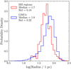 |
Fig. A.1 PDFs of the size of GMCs in blue and H II regions in red. Means, medians, and standard deviations of the two distributions are listed on the left. |
Appendix A.2: Asymmetry of the matching criterion
We are specifically looking for H II regions that may significantly modify the properties of their natal GMC clouds, not only at the immediate working surface, but also on the ~ 50 − 100 pc scales on which global cloud properties are typically measured. This implies that we are searching for H II regions whose energy content is a significant fraction of the GMC one. In particular, we explicitly tried to avoid selecting all the small H II regions associated with large GMCs because their feedback would have a negligible impact and they would dilute the searched signatures on the GMC properties.
For completeness, Fig. A.1 presents the PDFs of the radii of H II regions and GMCs across our sample. The size of resolved GMCs or H II regions are corrected for the size of ALMA and MUSE point spread function. But this plot should not be over-interpreted because the GMC and H II-region catalogs treat differently unresolved sources. The unresolved GMCs, on one hand, are filtered out from the PHANGS-ALMA catalog of GMCs, which rejects objects when their size cannot be deconvolved from the beam size (Rosolowsky et al. 2021). On the other hand, the majority (~ 80%) of the catalogued H II regions are point sources, for which we only have an upper limit of their projected area, corresponding to the point spread function of the VLT/MUSE instrument (Santoro et al. 2022). That is why the distribution of H II region size exhibits shallow peaks at the resolution of the observations, namely ~50 pc, ~60 pc and ~80 pc. Using these definitions, the 10 to 90 percentile range is 32 − 109 pc for the GMC radius, and 33 − 87 pc for the H II region radius. And there exist H II regions as large as the largest identified GMCs.
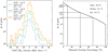 |
Fig. A.2 Histogram of the relative velocity (left) and number of pairs as a function of the MOP (right) between associated GMCs and H II regions for all galaxies in the sample. One GMC–H II region pair is present in this histogram when at least one pixel is overlapping. The mean, median, and standard deviation of the overlap distribution are listed on the top right corner. The vertical dashed lines in the right panel represent the 10%, 40% and 70% MOP. |
Appendix A.3: Overlap parameter choices
When matching GMCs and H II regions with the overlap matching method coupled with the velocity offset, two parameters are left to the user: the MOP and the velocity offset threshold. The left panel of Fig. A.2 presents the histogram of the number of GMC-H II region pairs as a function of their velocity offsets. Limiting the velocity offset between a spatially overlapping GMC and H II region ensures that the two objects are at least contiguous in position-position-velocity space. The uncertainty on the velocity of H II regions is ~ 49 km s−1, larger than the uncertainty on GMC velocity, and thus the limiting factor on the velocity offset threshold. We thus chose a velocity offset threshold of 10 km s−1. We note that limiting the velocity offset to a value lower than 10 km s−1, for example 5 km s−1, does not alter our results. As for the MOP, using 40% as a fiducial value allows us to filter out matched H II regions and GMCs that are potentially physically unrelated, while keeping a large enough sample of GMC-H II region pairs to compute reliable statistics. The right panel of Fig. A.2 presents the histogram of the number of GMC-H II region pairs according to the projected area of overlap. The distribution of overlap percentages between H II regions and GMCs has a mean of 17%, a median of 10%, and a standard deviation of 18%.
Appendix B Properties of the matched GMC–H II regions in individual galaxies
As an example, Fig. B.1 compares the spatial distribution of matched GMC–H II regions in NGC 4254 for a MOP of 40% with the spatial footprints of the full distributions of GMCs and H II regions, and the environment masks.
Table B.1 presents the statistics of matched GMC-H II regions for each galaxy in our sample. For three different MOP thresholds, we list total number of H II regions and GMCs in each galaxy, the percentage of H II regions and GMCs that are located in matched regions, and their absolute and relative contributions to each galaxy’s Hα and CO luminosities. Fig. B.2 shows the correlation between CO peak temperature and Hα luminosity considering H II region/GMC pairs from NGC 1672, NGC 4535, and NGC 4321 separately. These three galaxies harbor the highest correlation coefficient between CO peak temperature and Hα luminosity (R2 ≥ 0.5).
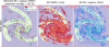 |
Fig. B.1 Comparison of the footprints of the matched GMCs/H II regions (left panel) with the footprints of all the GMCs (center panel) and of all the H II regions (right panel) for the NGC 4254 galaxy. The background image shows the Hα line emission in gray and the environmental masks: the center in yellow, the spiral arms in white, and the inter-arms and disk violet. In this case, regions are matched when the overlap area represents at least 40% of the GMC region area. |
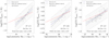 |
Fig. B.2 Scatter plots of the CO peak temperature as a function of the Hα luminosity for the 3 galaxies in our sample (NGC 1672, NGC4535, NGC4321) where these two properties are the most correlated. In this figure, the MOP is 40%. |
Number and luminosity of GMCs and H II regions per galaxy of the studied sample as a function of the MOP.
Appendix C Supplemental information to assess the robustness of the results
Kolmogorov-Smirnov tests performed to assess whether the distributions are significantly different. Top: Comparison of the distributions of matched GMC–H II regions with their parent distributions. Bottom: Comparison of the distributions of matched GMC–H II regions for different minimum overlap percentages.
Anderson-Darling tests performed to assess whether the distributions are significantly different. Top: Comparison of the distributions of matched GMC–H II regions with their parent distributions. Bottom: Comparison of the distributions of matched GMC–H II regions for different minimum overlap percentages.
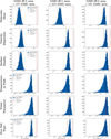 |
Fig. C.1 Histograms of the R2 coefficient between the different GMC properties and the Hα luminosity, after shuffling the Hα luminosity values, for three different minimum overlap percentage of the H II-GMC pairs: 10% for the left column, 40% for the middle one, and 70% for the right one. The solid lines show the mean of the distribution and the dotted lines the 1 standard deviation interval around the mean. |
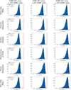 |
Fig. C.2 Histograms of the R2 coefficient between the different GMC properties and the Hα luminosity, after shuffling the Hα luminosity values while keeping the relationship between Hα luminosity and H II region radius values, for three different MOP of the H II-GMC pairs: 10% for the left column, 40% for the middle one, and 70% for the right one. The solid lines show the mean of the distribution and the dotted lines the 1 standard deviation interval around the mean. |
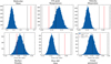 |
Fig. C.3 Bootstrap tests of the significance of the power-law index change with the MOP. The red line represents the power-law index obtained after matching with a 70% overlap, and the dashed lines its confidence interval. The blue distribution represents the power-law indices obtained after randomly sampling N pairs from the parent distribution (10% overlap), where N is the size of the 70% minimal overlap distribution. This random sampling has been performed 10000 times in order to obtain the distribution. This figure shows that the change in power-law index with the MOP cannot arise from a random sampling of the parent population, except for the surface density. |
Appendix D Supplemental figures about the variability of the properties of the matched GMC–H II regions as a function of the galaxy
Figures D.1 and D.2 respectively present the correlations coefficients and power-law indices of the correlation between the GMC peak brightness and the H II region Hα luminosity, as a function of different galaxy-wide properties. The properties in question are: the total number of matched GMC-H II regions, the galaxy’s distance, inclination, stellar mass, total CO luminosity, total Hα luminosity, mean stellar density environment and distance from the main sequence. For these figures the MOP is 40%. Reassuringly, the galaxy’s distance, inclination or number of matched GMC-H II regions does not have any impact on the found correlations.
To be more quantitative about the effect of inclination and metallicity, we computed a linear regression of the correlation coefficient R2 (of the peak temperature correlation with Hα luminosity) against the galaxies inclinations, total CO luminosities and metallicities. This will allow us to check whether a galactic property has a significant impact on the correlations or not.
For the linear regression between R2 and the galaxy inclination, the resulting correlation coefficient and slope are respectively 0.07 ± 0.08 and 0.004 ± 0.009. These numbers are consistent with 0, so the galaxy inclination has no impact on the correlations. For the linear regression between R2 and the galaxy metallicity, the resulting correlation coefficient and slope are respectively 0.15 ± 0.18 and 0.89 ± 1.15. These numbers are also consistent with 0, so the galaxy metallicity has no impact on the correlations. For comparison, the linear regression between R2 and the galaxy’s total CO luminosity yields a correlation coefficient and a slope of respectively 0.32 ± 0.13 and 0.16 ± 0.06.
Correlation properties (R2 coefficient and power-law index) for various GMC properties as a function of the Hα luminosity for each galaxy in the sample. The minimum overlap percentage used for the matching is 40%. The galaxies are sorted by decreasing R2 coefficient for each individual sub-table.
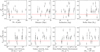 |
Fig. D.1 R2 coefficients of the temperature at peak with the Hα luminosity considering H II region/GMC pairs from each galaxy in the sample separately. Top from left to right: R2 coefficients versus the number of matched H II regions and GMCs, distance, inclination and total stellar mass of the host galaxy. Bottom from left to right: R2 coefficients versus the galaxy’s CO luminosity, total Hα luminosity, average stellar surface density within a 500 pc radius around each of the H II region/GMC pairs and the galaxy’s offset from the main sequence. The red dashed line shows the global R2 coefficient from Sect. 5. |
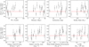 |
Fig. D.2 Same as figure D.1 but the R2 values are replaced by the power-law indices. |
Appendix E Supplemental information about the covariations of GMC properties
The evolution of the correlations of the GMC properties with the Hα luminosity of the associated H II regions show two different trends. It is well known that GMC properties covary through Larson’s and Heyer’s relationships (Heyer & Brunt 2004; Larson 1981). We ask here which part of the uncovered trends are controlled by these covariations of the GMC properties.
Figure E.1 shows the joint PDFs of the quantities that are known to covary in our sample (Rosolowsky et al. 2021).
Larson’s first relationship links the GMC velocity dispersion to its radius through
 (E.1)
(E.1)
Larson’s second relationship links the GMC velocity dispersion to its mass through
 (E.2)
(E.2)
Heyer’s relationship links the characteristic turbulent linewidth to the surface density through
 (E.3)
(E.3)
Moreover, Fig E 1 shows that all these power-law relations are stable within the credibility intervals when increasing the MOP. Unlike the correlations between different GMC properties and the H II region luminosity, Larson’s and Heyer’s relationships as well as the correlation between the CO peak temperature and the molecular surface density are insensitive to the minimum overlap percentage, especially in terms of power-law index.
The similar evolution with the MOP of the correlations of the molecular surface density, CO peak temperature, and characteristic turbulent linewidth with the Hα luminosity leads us to ask whether there is an additional covariation between the CO peak temperature and the molecular surface density. Indeed, Fig. E.1 suggests that there is a relationship, even though imperfect, through
 (E.4)
(E.4)
Figure E.2 shows the evolution of the joint PDF of the CO peak temperature and the GMC mass with the minimum overlap percentage. We find a positive correlation
 (E.5)
(E.5)
with a R2 value of 0.27. This positive correlation implies that the two behaviors uncovered between the GMC properties and the Hα luminosities are independent. Indeed, an anticorrelation between the CO peak temperature and the GMC mass is needed to explain the shift of the marginalized PDF of these two quantities in opposite directions. In other words, the presence of an H II region more or less close to its parent GMC modifies some of the intrinsic scaling relationships between GMC properties.
 |
Fig. E.1 Evolution of the Larson, Heyer, and peak temperature versus surface density correlations for all the GMCs in the sample (first columns) and three different minimum overlap percentage of the H II-GMC pairs: 10% for the second column, 40% for the third one, and 70% for the fourth one. The solid and dotted black lines show the power-law fits and their uncertainty, respectively. The dashed lines show the ±3σ levels from the fitted line. The power-law parameters are displayed on the bottom-right corner of each panel. The red solid lines show the power-law fit for the parent population (all GMCs in the sample). |
 |
Fig. E.2 Evolution of the joint PDF between the peak temperature (top) and the characteristic turbulent linewidth (bottom), and the molecular mass for all the GMCs in the sample (first columns) and three different MOPs of the H II–GMC pairs: 10% for the second column, 40% for the third one, and 70% for the fourth. The reminder of the layout is similar to Fig. E.1. |
References
- Anand, G. S., Lee, J. C., Van Dyk, S. D., et al. 2021, MNRAS, 501, 3621 [Google Scholar]
- Bacon, R., Accardo, M., Adjali, L., et al. 2010, SPIE Conf. Ser., 7735, 773508 [Google Scholar]
- Bacon, R., Conseil, S., Mary, D., et al. 2017, A & A, 608, A1 [NASA ADS] [CrossRef] [EDP Sciences] [Google Scholar]
- Barnes, A. T., Longmore, S. N., Dale, J. E., et al. 2020, MNRAS, 498, 4906 [NASA ADS] [CrossRef] [Google Scholar]
- Barnes, A. T., Glover, S. C. O., Kreckel, K., et al. 2021, MNRAS, 508, 5362 [NASA ADS] [CrossRef] [Google Scholar]
- Barnes, A. T., Chandar, R., Kreckel, K., et al. 2022, A & A, 662, A6 [Google Scholar]
- Bolatto, A. D., Warren, S. R., Leroy, A. K., et al. 2013, Nature, 499, 450 [Google Scholar]
- Chevance, M., Kruijssen, J. M. D., Hygate, A. P. S., et al. 2020, MNRAS, 493, 2872 [NASA ADS] [CrossRef] [Google Scholar]
- Chevance, M., Kruijssen, J. M. D., Krumholz, M. R., et al. 2022, MNRAS, 509, 272 [Google Scholar]
- Chevance, M., Krumholz, M. R., McLeod, A. F., et al. 2023, ASP Conf. Ser., 534, 1 [NASA ADS] [Google Scholar]
- Emsellem, E., Schinnerer, E., Santoro, F., et al. 2022, A & A, 659, A191 [NASA ADS] [CrossRef] [EDP Sciences] [Google Scholar]
- Fujimoto, Y., Bryan, G. L., Tasker, E. J., Habe, A., & Simpson, C. M. 2016, MNRAS, 461, 1684 [NASA ADS] [CrossRef] [Google Scholar]
- Grasha, K., Calzetti, D., Bittle, L., et al. 2018, MNRAS, 481, 1016 [NASA ADS] [CrossRef] [Google Scholar]
- Grasha, K., Calzetti, D., Adamo, A., et al. 2019, MNRAS, 483, 4707 [NASA ADS] [CrossRef] [Google Scholar]
- Großschedl, J. E., Alves, J., Meingast, S., & Herbst-Kiss, G. 2021, A & A, 647, A91 [CrossRef] [EDP Sciences] [Google Scholar]
- Groves, B., Kreckel, K., Santoro, F., et al. 2023, MNRAS, 520, 4902 [Google Scholar]
- Grudić, M. Y., Hopkins, P. F., Lee, E. J., et al. 2019, MNRAS, 488, 1501 [CrossRef] [Google Scholar]
- Herrera, C. N., Pety, J., Hughes, A., et al. 2020, A & A, 634, A121 [CrossRef] [EDP Sciences] [Google Scholar]
- Heyer, M. H., & Brunt, C. M. 2004, ApJ, 615, L45 [NASA ADS] [CrossRef] [Google Scholar]
- Hopkins, P. F., Quataert, E., & Murray, N. 2012, MNRAS, 421, 3522 [Google Scholar]
- Kauffmann, G., Heckman, T. M., Tremonti, C., et al. 2003, MNRAS, 346, 1055 [Google Scholar]
- Kewley, L. J., Heisler, C. A., Dopita, M. A., & Lumsden, S. 2001, ApJS, 132, 37 [Google Scholar]
- Kim, J., Chevance, M., Kruijssen, J. M. D., et al. 2021a, MNRAS, 504, 487 [NASA ADS] [CrossRef] [Google Scholar]
- Kim, J.-G., Ostriker, E. C., & Filippova, N. 2021b, ApJ, 911, 128 [NASA ADS] [CrossRef] [Google Scholar]
- Kim, J., Chevance, M., Kruijssen, J. M. D., et al. 2022, MNRAS, 516, 3006 [NASA ADS] [CrossRef] [Google Scholar]
- Kreckel, K., Faesi, C., Kruijssen, J. M. D., et al. 2018, ApJ, 863, L21 [NASA ADS] [CrossRef] [Google Scholar]
- Kruijssen, J. M. D., Schruba, A., Hygate, A. P. S., et al. 2018, MNRAS, 479, 1866 [NASA ADS] [CrossRef] [Google Scholar]
- Kruijssen, J. M. D., Schruba, A., Chevance, M., et al. 2019, Nature, 569, 519 [NASA ADS] [CrossRef] [Google Scholar]
- Krumholz, M. R. 2014, Phys. Rep., 539, 49 [Google Scholar]
- Krumholz, M. R., McKee, C. F., & Bland-Hawthorn, J. 2019, ARA & A, 57, 227 [NASA ADS] [CrossRef] [Google Scholar]
- Lang, P., Meidt, S. E., Rosolowsky, E., et al. 2020, ApJ, 897, 122 [CrossRef] [Google Scholar]
- Larson, R. B. 1981, MNRAS, 194, 809 [Google Scholar]
- Leroy, A. K., Hughes, A., Liu, D., et al. 2021a, ApJS, 255, 19 [NASA ADS] [CrossRef] [Google Scholar]
- Leroy, A. K., Schinnerer, E., Hughes, A., et al. 2021b, ApJS, 257, 43 [NASA ADS] [CrossRef] [Google Scholar]
- Lopez, L. A., Krumholz, M. R., Bolatto, A. D., Prochaska, J. X., & Ramirez-Ruiz, E. 2011, ApJ, 731, 91 [Google Scholar]
- Lopez, L. A., Krumholz, M. R., Bolatto, A. D., et al. 2014, ApJ, 795, 121 [NASA ADS] [CrossRef] [Google Scholar]
- Luisi, M., Anderson, L. D., Schneider, N., et al. 2021, Sci. Adv., 7, eabe9511 [NASA ADS] [CrossRef] [Google Scholar]
- Malhotra, S. 1994, ApJ, 433, 687 [NASA ADS] [CrossRef] [Google Scholar]
- McLeod, A. F., Reiter, M., Kuiper, R., Klaassen, P. D., & Evans, C. J. 2018, Nature, 554, 334 [CrossRef] [Google Scholar]
- McLeod, A. F., Dale, J. E., Evans, C. J., et al. 2019, MNRAS, 486, 5263 [Google Scholar]
- McLeod, A. F., Kruijssen, J. M. D., Weisz, D. R., et al. 2020, ApJ, 891, 25 [NASA ADS] [CrossRef] [Google Scholar]
- McLeod, A. F., Ali, A. A., Chevance, M., et al. 2021, MNRAS, 508, 5425 [NASA ADS] [CrossRef] [Google Scholar]
- O’Donnell, J. E. 1994, ApJ, 422, 158 [Google Scholar]
- Olivier, G. M., Lopez, L. A., Rosen, A. L., et al. 2021, ApJ, 908, 68 [NASA ADS] [CrossRef] [Google Scholar]
- Onodera, S., Kuno, N., Tosaki, T., et al. 2010, ApJ, 722, L127 [NASA ADS] [CrossRef] [Google Scholar]
- Pabst, C., Higgins, R., Goicoechea, J. R., et al. 2019, Nature, 565, 618 [NASA ADS] [CrossRef] [Google Scholar]
- Pan, H.-A., Schinnerer, E., Hughes, A., et al. 2022, ApJ, 927, 9 [NASA ADS] [CrossRef] [Google Scholar]
- Pilyugin, L. S., & Grebel, E. K. 2016, MNRAS, 457, 3678 [NASA ADS] [CrossRef] [Google Scholar]
- Rosolowsky, E., & Leroy, A. 2006, PASP, 118, 590 [NASA ADS] [CrossRef] [Google Scholar]
- Rosolowsky, E., Hughes, A., Leroy, A. K., et al. 2021, MNRAS, 502, 1218 [NASA ADS] [CrossRef] [Google Scholar]
- Sánchez, S. F., Rosales-Ortega, F. F., Iglesias-Páramo, J., et al. 2014, A & A, 563, A49 [CrossRef] [EDP Sciences] [Google Scholar]
- Sánchez, S. F., Barrera-Ballesteros, J. K., López-Cobá, C., et al. 2019, MNRAS, 484, 3042 [CrossRef] [Google Scholar]
- Santoro, F., Kreckel, K., Belfiore, F., et al. 2022, A & A, 658, A188 [NASA ADS] [CrossRef] [EDP Sciences] [Google Scholar]
- Schaye, J., Crain, R. A., Bower, R. G., et al. 2015, MNRAS, 446, 521 [Google Scholar]
- Schinnerer, E., Meidt, S. E., Colombo, D., et al. 2017, ApJ, 836, 62 [NASA ADS] [CrossRef] [Google Scholar]
- Schinnerer, E., Hughes, A., Leroy, A., et al. 2019, ApJ, 887, 49 [NASA ADS] [CrossRef] [Google Scholar]
- Schlafly, E. F., & Finkbeiner, D. P. 2011, ApJ, 737, 103 [Google Scholar]
- Schruba, A., Leroy, A. K., Walter, F., Sandstrom, K., & Rosolowsky, E. 2010, ApJ, 722, 1699 [NASA ADS] [CrossRef] [Google Scholar]
- Sun, J., Leroy, A. K., Schinnerer, E., et al. 2020, ApJ, 901, L8 [NASA ADS] [CrossRef] [Google Scholar]
- Sun, J., Leroy, A. K., Rosolowsky, E., et al. 2022, AJ, 164, 43 [NASA ADS] [CrossRef] [Google Scholar]
- Thilker, D. A., Braun, R., & Walterbos, R. A. M. 2000, AJ, 120, 3070 [Google Scholar]
- Utomo, D., Sun, J., Leroy, A. K., et al. 2018, ApJ, 861, L18 [NASA ADS] [CrossRef] [Google Scholar]
- Watkins, E. J., Peretto, N., Marsh, K., & Fuller, G. A. 2019, A & A, 628, A21 [NASA ADS] [CrossRef] [EDP Sciences] [Google Scholar]
- Williams, J. P., & McKee, C. F. 1997, ApJ, 476, 166 [NASA ADS] [CrossRef] [Google Scholar]
All Tables
Fraction of GMCs and H II regions that are identified as matched objects across our sample.
Number and luminosity of GMCs and H II regions per galactic environment of the studied sample, for a MOP of 40%.
Number and luminosity of GMCs and H II regions per galaxy of the studied sample as a function of the MOP.
Kolmogorov-Smirnov tests performed to assess whether the distributions are significantly different. Top: Comparison of the distributions of matched GMC–H II regions with their parent distributions. Bottom: Comparison of the distributions of matched GMC–H II regions for different minimum overlap percentages.
Anderson-Darling tests performed to assess whether the distributions are significantly different. Top: Comparison of the distributions of matched GMC–H II regions with their parent distributions. Bottom: Comparison of the distributions of matched GMC–H II regions for different minimum overlap percentages.
Correlation properties (R2 coefficient and power-law index) for various GMC properties as a function of the Hα luminosity for each galaxy in the sample. The minimum overlap percentage used for the matching is 40%. The galaxies are sorted by decreasing R2 coefficient for each individual sub-table.
All Figures
|
Fig. 1 Example results of the algorithm used to match GMCs (blue) and H II regions (red) for the same field of view. The background image is Hα line emission from a spiral arm segment in NGC 4254. The right and left panels show the matches obtained when the area of the GMC–H II region overlap is at least 10% and 70%, respectively, of the projected area of a GMC. Imposing a higher overlap percentage leads to fewer identifications of matched GMC–H II regions. |
| In the text | |
|
Fig. 2 PDFs of key physical properties of H II regions and of GMCs. Top, from left to right: Extinction-corrected Hα luminosity and size. Bottom, from top left to bottom right: CO luminosity, size, peak temperature, velocity dispersion, surface density, characteristic turbulent linewidth, free-fall time, and virial parameter. The distribution for the full GMC (H II region) population is shown in red, while the matched GMCs–H II regions adopting a MOP of 10, 40, and 70% are shown in blue, green, and gold, respectively. |
| In the text | |
|
Fig. 3 Correlation matrix of the different GMC and H II region properties investigated. The top-left blue square shows the correlations between GMC properties considering the entire sample. The bottom-right red square shows the correlations between the properties of H II regions considering the entire sample. The bottom-left black rectangle shows the strengths of the correlations between matched GMC and H II regions for a MOP of 70%. |
| In the text | |
|
Fig. 4 Scatter plots of various GMC properties as a function of the Hα luminosity for three different MOPs of the H II–GMC pairs: 10% for the left column, 40% for the middle one, and 70% for the right one. The GMC properties are, from top to bottom: the molecular mass, the characteristic turbulent linewidth, the surface density, and the peak temperature. The solid black lines show a power-law fit and its uncertainty for each scatter plot. The dashed lines show the ±3σ levels from the fitted line. The solid red line represents the linear regressions obtained in the leftmost column, for comparison. The fitted line properties are displayed at the bottom-right corner of each panel. |
| In the text | |
|
Fig. 5 R2 (top) and power-law index (bottom) of the fits of various GMC properties (as a function of the Hα luminosity of the matched H II region) against the MOP. The fitted GMC properties are, from left to right: the molecular mass, the peak temperature, the surface density, and the characteristic turbulent linewidth. Blue (respectively red) lines show an increase (respectively decrease) of the R2 coefficient with the MOP. The uncertainty intervals are computed using a standard bootstrap method. |
| In the text | |
|
Fig. 6 PDFs of the stellar mass surface density within 500 pc of the matched GMC–H II regions. The global population in shown in red, and the matched population, with a MOP of 40%, in shown in black. The vertical dashed lines show the limits used to define the three stellar density environments in Sect. 6. |
| In the text | |
|
Fig. 7 Fraction of GMC-H II region pairs with low, medium, or high density environments in the galaxies’ center (nucleus and bar), arms, and disk (interarms and outer disk), for a MOP of 40%. |
| In the text | |
|
Fig. 8 Scatter plots of various GMC properties as a function of the Hα luminosity for different environmental stellar surface densities measured at a scale of 500 pc, in a similar fashion to Fig. 4. Each column represents a bin of environmental stellar surface density, as defined in Sect. 6. From left to right: low density, average density, and high density environments. The red line shows the global correlation from Sect. 5 with a MOP of 40%. |
| In the text | |
|
Fig. 9 Joint PDFs and their marginalized PDFs of the GMCs peak temperature (left) and molecular mass (right) with the matched H II region Hα luminosity for two MOPs: 1% in red and 70% in blue. The joint PDFs are shown as contour plots. The medians of the marginalized PDFs and the power laws fitted on the joint PDFs are overlaid as straight lines. |
| In the text | |
|
Fig. A.1 PDFs of the size of GMCs in blue and H II regions in red. Means, medians, and standard deviations of the two distributions are listed on the left. |
| In the text | |
|
Fig. A.2 Histogram of the relative velocity (left) and number of pairs as a function of the MOP (right) between associated GMCs and H II regions for all galaxies in the sample. One GMC–H II region pair is present in this histogram when at least one pixel is overlapping. The mean, median, and standard deviation of the overlap distribution are listed on the top right corner. The vertical dashed lines in the right panel represent the 10%, 40% and 70% MOP. |
| In the text | |
|
Fig. B.1 Comparison of the footprints of the matched GMCs/H II regions (left panel) with the footprints of all the GMCs (center panel) and of all the H II regions (right panel) for the NGC 4254 galaxy. The background image shows the Hα line emission in gray and the environmental masks: the center in yellow, the spiral arms in white, and the inter-arms and disk violet. In this case, regions are matched when the overlap area represents at least 40% of the GMC region area. |
| In the text | |
|
Fig. B.2 Scatter plots of the CO peak temperature as a function of the Hα luminosity for the 3 galaxies in our sample (NGC 1672, NGC4535, NGC4321) where these two properties are the most correlated. In this figure, the MOP is 40%. |
| In the text | |
|
Fig. C.1 Histograms of the R2 coefficient between the different GMC properties and the Hα luminosity, after shuffling the Hα luminosity values, for three different minimum overlap percentage of the H II-GMC pairs: 10% for the left column, 40% for the middle one, and 70% for the right one. The solid lines show the mean of the distribution and the dotted lines the 1 standard deviation interval around the mean. |
| In the text | |
|
Fig. C.2 Histograms of the R2 coefficient between the different GMC properties and the Hα luminosity, after shuffling the Hα luminosity values while keeping the relationship between Hα luminosity and H II region radius values, for three different MOP of the H II-GMC pairs: 10% for the left column, 40% for the middle one, and 70% for the right one. The solid lines show the mean of the distribution and the dotted lines the 1 standard deviation interval around the mean. |
| In the text | |
|
Fig. C.3 Bootstrap tests of the significance of the power-law index change with the MOP. The red line represents the power-law index obtained after matching with a 70% overlap, and the dashed lines its confidence interval. The blue distribution represents the power-law indices obtained after randomly sampling N pairs from the parent distribution (10% overlap), where N is the size of the 70% minimal overlap distribution. This random sampling has been performed 10000 times in order to obtain the distribution. This figure shows that the change in power-law index with the MOP cannot arise from a random sampling of the parent population, except for the surface density. |
| In the text | |
|
Fig. D.1 R2 coefficients of the temperature at peak with the Hα luminosity considering H II region/GMC pairs from each galaxy in the sample separately. Top from left to right: R2 coefficients versus the number of matched H II regions and GMCs, distance, inclination and total stellar mass of the host galaxy. Bottom from left to right: R2 coefficients versus the galaxy’s CO luminosity, total Hα luminosity, average stellar surface density within a 500 pc radius around each of the H II region/GMC pairs and the galaxy’s offset from the main sequence. The red dashed line shows the global R2 coefficient from Sect. 5. |
| In the text | |
|
Fig. D.2 Same as figure D.1 but the R2 values are replaced by the power-law indices. |
| In the text | |
|
Fig. E.1 Evolution of the Larson, Heyer, and peak temperature versus surface density correlations for all the GMCs in the sample (first columns) and three different minimum overlap percentage of the H II-GMC pairs: 10% for the second column, 40% for the third one, and 70% for the fourth one. The solid and dotted black lines show the power-law fits and their uncertainty, respectively. The dashed lines show the ±3σ levels from the fitted line. The power-law parameters are displayed on the bottom-right corner of each panel. The red solid lines show the power-law fit for the parent population (all GMCs in the sample). |
| In the text | |
|
Fig. E.2 Evolution of the joint PDF between the peak temperature (top) and the characteristic turbulent linewidth (bottom), and the molecular mass for all the GMCs in the sample (first columns) and three different MOPs of the H II–GMC pairs: 10% for the second column, 40% for the third one, and 70% for the fourth. The reminder of the layout is similar to Fig. E.1. |
| In the text | |
Current usage metrics show cumulative count of Article Views (full-text article views including HTML views, PDF and ePub downloads, according to the available data) and Abstracts Views on Vision4Press platform.
Data correspond to usage on the plateform after 2015. The current usage metrics is available 48-96 hours after online publication and is updated daily on week days.
Initial download of the metrics may take a while.