| Issue |
A&A
Volume 677, September 2023
|
|
|---|---|---|
| Article Number | A106 | |
| Number of page(s) | 21 | |
| Section | Interstellar and circumstellar matter | |
| DOI | https://doi.org/10.1051/0004-6361/202347077 | |
| Published online | 13 September 2023 | |
Abundance and excitation of molecular anions in interstellar clouds★
1
Instituto de Física Fundamental, CSIC,
Calle Serrano 123,
28006
Madrid,
Spain
e-mail: This email address is being protected from spambots. You need JavaScript enabled to view it.
2
Observatorio Astronómico Nacional, IGN,
Calle Alfonso XII 3,
28014
Madrid,
Spain
3
Observatorio de Yebes, IGN,
Cerro de la Palera s/n,
19141
Yebes, Guadalajara,
Spain
4
Centro de Astrobiología (CSIC/INTA),
Ctra. de Torrejón a Ajalvir km 4,
28806
Torrejón de Ardoz,
Spain
Received:
2
June
2023
Accepted:
6
July
2023
Abstract
We present new observations of molecular anions with the Yebes 40 m and IRAM 30 m telescopes toward the cold, dense clouds TMC-1 CP, Lupus-1A, L1527, L483, L1495B, and L1544. We report the first detections of C3N− and C5N− in Lupus-1A as well as C4H− and C6H− in L483. In addition, we detected new lines of C6H− toward the six targeted sources, of C4H− toward TMC-1 CP, Lupus-1A, and L1527, and of C8H− and C3N− in TMC-1 CP. Excitation calculations using recently computed collision rate coefficients indicate that the lines of anions accessible to radiotelescopes run from subthermally excited to thermalized as the size of the anion increases, with the degree of departure from thermalization depending on the H2 volume density and the line frequency. We noticed that the collision rate coefficients available for the radical C6H are not sufficient to explain various observational facts, thereby calling for the collision data for this species to be revisited. The observations presented here, together with observational data from the literature, have been used to model the excitation of interstellar anions and to constrain their abundances. In general, the anion-to-neutral ratios derived here agree with the literature values, when available, within 50% (by a factor of two at most), except for the C4H−/C4H ratio, which shows higher differences due to a revision of the dipole moment of C4H. From the set of anion-to-neutral abundance ratios derived two conclusions can be drawn. First, the C6H−/C6H ratio shows a tentative trend whereby it increases with increasing H2 density, as we would expect on the basis of theoretical grounds. Second, the assertion that the higher the molecular size, the higher the anion-to-neutral ratio is incontestable; furthermore, this supports a formation mechanism based on radiative electron attachment. Nonetheless, the calculated rate coefficients for electron attachment to the medium size species C4H and C3N are probably too high and too low, respectively, by more than one order of magnitude.
Key words: astrochemistry / line: identification / molecular processes / radiative transfer / ISM: molecules / radio lines: ISM
Based on observations carried out with the Yebes 40 m telescope (projects 19A003, 20A014, 20A016, 20B010, 20D023, 21A006, 21A011, 21D005, 22B023, and 23A024) and the IRAM 30 m telescope. The 40 m radio telescope at Yebes Observatory is operated by the Spanish Geographic Institute (IGN; Ministerio de Transportes, Movilidad y Agenda Urbana). IRAM is supported by INSU/CNRS (France), MPG (Germany), and IGN (Spain).
© The Authors 2023
 Open Access article, published by EDP Sciences, under the terms of the Creative Commons Attribution License (https://creativecommons.org/licenses/by/4.0), which permits unrestricted use, distribution, and reproduction in any medium, provided the original work is properly cited.
This article is published in open access under the Subscribe to Open model. This email address is being protected from spambots. You need JavaScript enabled to view it. to support open access publication.
1 Introduction
The discovery of negatively charged molecular ions in space has been a relatively recent finding (McCarthy et al. 2006). To date, the inventory of molecular anions detected in interstellar and circumstellar clouds consists of four hydrocarbon anions: C4H− (Cernicharo et al. 2007), C6H− (McCarthy et al. 2006), C8H− (Brünken et al. 2007a; Remijan et al. 2007), and C1oH− (Remijan et al. 2023), as well as four nitrile anions, CN− (Agúndez et al. 2010), C3N− (Thaddeus et al. 2008), C5N− (Cernicharo et al. 2008), and C7N− (Cernicharo et al. 2023a). The astronomical detection of most of these species has been possible thanks to the laboratory characterization of their rotational spectrum (McCarthy et al. 2006; Gupta et al. 2007; Gottlieb et al. 2007; Thaddeus et al. 2008). However, the astronomical detection of C5N−, C7N−, and C10H− is based on high-level ab initio calculations and astrochemical arguments (Botschwina & Oswald 2008; Cernicharo et al. 2008, 2020, 2023a; Remijan et al. 2023). In fact, in the case of C10H− it is not yet clear whether the identified species is C10H− or C9N− (Pardo et al. 2023).
The current situation is such that there is only one astronomical source where the eight molecular anions have been observed, the carbon-rich circumstellar envelope IRC + 10216 (McCarthy et al. 2006; Cernicharo et al. 2007, 2008, 2023a; 2007; Thaddeus et al. 2008; Agúndez et al. 2010; Pardo et al. 2023), while the first negative ion discovered, C6H− (McCarthy et al. 2006), continues to be the most widely observed in astronomical sources (Sakai et al. 2007, 2010; Gupta et al. 2009; Cordiner et al. 2011, 2013).
Observations indicate that along each of the series C2n+2H− and C2n−1 N− (with n = 1, 2, 3, and 4), the anion-to-neutral abundanceratio increases with increasing molecularsize (Millar et al. 2017). This is expected according to the formation mechanism originally proposed by Herbst (1981), which involves the radiative electron attachment to the neutral counterpart of the anion (Herbst & Osamura 2008; Carelli et al. 2013). However, the efficiency of this mechanism in interstellar space has been disputed (Khamesian et al. 2016) and alternative formation mechanisms have been proposed (Gianturco et al. 2016). As yet, there is no consensus on the formation mechanism of molecular anions in space (see discussion in Millar et al. 2017). Moreover, detections of negative ions other than C6H− in interstellar clouds are scarce; thus, our view of the abundance of the different anions in interstellar space is statistically very limited.
Apart from the anion-to-anion behavior, it is also interesting to know which is the source-to-source behavior. That is to say, we consider how the abundance of anions behaves from one source to another. Based on C6H− detections, the C6H−/C6H abundance ratio seems to increase with increasing H2 volume density (Sakai et al. 2007; Agúndez et al. 2008; Cordiner et al. 2013), which is expected from chemical considerations (e.g., Flower et al. 2007; see also Sect. 6). However, most anion detections in interstellar clouds have been based on one or two lines and their abundances have been estimated assuming that their rotational levels are populated according to local thermodynamic equilibrium (LTE), which may not be a good assumption given the large dipole moments, and thus high critical densities, of anions. Recently, rate coefficients for inelastic collisions with H2 or He have been calculated for C2H− (Dumouchel et al. 2012, 2023; Gianturco et al. 2019; Franz et al. 2020; Toumi et al. 2021), C4H− (Senent et al. 2019; Balança et al. 2021), C6H− (Walker et al. 2016, 2017), CN− (Kłos & Lique 2011; González-Sánchez et al. 2020), C3N− (Lara-Moreno et al. 2017, 2019; Tchakoua et al. 2018), and C5N− (Biswas et al. 2023), which makes it possible to study the excitation of anions in the interstellar medium.
Here, we report new detections of anions in interstellar sources. Concretely, we detected C3N− and C5N− in Lupus-1A and C6H− and C4H− in L483. We also present the detection of new lines of C4H−, C6H−, C8H−, C3N−, and C5N− in interstellar clouds where these anions have been already observed. We use the large observational dataset from this study, together with that available from the literature, to review the observational status of anions in interstellar clouds and to carry out a comprehensive analysis of the abundance and excitation of anions in the interstellar medium.
2 Observations
2.1 Yebes 40 m and IRAM 30 m observations from this study
The observations of cold dark clouds presented in this study were carried out with the Yebes40m and IRAM30m telescopes. We targeted the starless core TMC-1 at the cyanopolyyne peak position (hereafter, TMC-1 CP)1, the starless core Lupus-1A2, the prestellar cores L1495B3 and L15444, and the dense cores L15275 and L4836, which host a Class 0 protostar. All observations were done using the frequency switching technique to maximize the on-source telescope time and to improve the sensitivity of the spectra.
The Yebes 40 m observations consisted in a full scan of the Q band (31–50 GHz) acquired in a single spectral setup with a 7 mm receiver, which was connected to a fast Fourier transform spectrometer that provides a spectral resolution of 38 kHz (Tercero et al. 2021). The data of TMC-1 CP are part of the on-going QUIJOTE line survey (Cernicharo et al. 2021). The spectra used here were obtained between November 2019 and November 2022, comprising a total of 758 h of on-source telescope time in each polarization (twice this value after averaging both polarizations). Two frequency throws of 8 and 10 MHz were used. The sensitivity ranges from 0.13 to 0.4 mK in antenna temperature. The data of L1544 were taken between October and December 2020 toward the position of the methanol peak of this core, where complex organic molecules have been detected (Jiménez-Serra et al. 2016), and are part of a high-sensitivity Q-band survey (31 h on-source; Jiménez-Serra et al., in prep.). The data for the other sources were obtained from July 2020 to February 2023 for L483 (the total on-source telescope time is 103 h), from May to November 2021 for L1527 (40 h on-source), from July 2021 to January 2023 for Lupus-1A (120 h on-source), and from September to November 2021 for L1495B (45 h on-source). Different frequency throws were adopted depending on the observing period, which resulted from tests done at the Yebes 40 m telescope to find the optimal frequency throw. We applied frequency throws of 10 MHz and 10.52 MHz for L483, 10 MHz for L1544, 8 MHz for L1527, and 10.52 MHz for Lupus-1A and L1495B. The antenna temperature noise levels, after averaging horizontal and vertical polarizations, are in the range of 0.4–1.0 mK for L483, 1.3–1.8 mK for L1544, 0.7–2.7 mK for L1527, 0.7–2.8 mK for Lupus-1A, and 0.8–2.6 mK for L1495B.
The observations carried out with the IRAM 30 m telescope used the 3 mm EMIR receiver connected to a fast Fourier transform spectrometer that provides a spectral resolution of 49 kHz. Different spectral regions within the 3 mm band (72–116 GHz) were covered depending on the source. The data of TMC-1 CP consist of a 3 mm line survey (Marcelino et al. 2007; Cernicharo et al. 2012) and spectra observed in 2021 (Agúndez et al. 2022; Cabezas et al. 2022). The data of L483 consist of a line survey in the 80–116 GHz region (see Agúndez et al. 2019), together with data in the 72–80 GHz region, which are described in Cabezas et al. (2021). Data of Lupus-1A, L1495B, L1521F, L1251A, L1512, L1172, and L1389 were observed from September to November 2014 during a previous search for molecular anions at mm wavelengths (see Agúndez et al. 2015). Additional data on Lupus-1A were gathered during 2021 and 2022 during a project aimed to observe H2NC (Agúndez et al. 2023). In the case of L1527, the IRAM 30 m data used were observed in July and August 2007 with the old ABCD receivers connected to an autocorrelator that provided spectral resolutions of 40 or 80 kHz (Agúndez et al. 2008).
The half power beam width (HPBW) of the Yebes 40 m telescope is in the range 35–57″ in the Q band, while that of the IRAM 30 m telescope ranges between 21″ and 34″ in the 3 mm band. The beam size can be fitted as a function of frequency as HPBW(″) = 1763/ν(GHz) for the Yebes 40 m telescope and as HPBW(″) = 2460/ν(GHz) for the IRAM30m telescope. Therefore, the beam size of the IRAM30m telescope at 72 GHz is similar to that of the Yebes 40 m at 50 GHz. The intensity scale in both the Yebes 40 m and IRAM 30 m telescopes is antenna temperature,  , for which we estimate a calibration error of 10%. To convert antenna temperature into main beam brightness temperature see foot of Table A.1. All data were analyzed using the CLASS program of the GILDAS software7.
2.2 Observational dataset of anions in dark clouds
In Table A.1, we compile the line parameters of all the lines of negative molecular ions detected toward cold dark clouds, including those from this study and from the literature. The line parameters of C7N− observed toward TMC-1 CP are given in Cernicharo et al. (2023a) and are not repeated here. In the case of C10H− in TMC-1 CP, we do not include line parameters here because the detection by Remijan et al. (2023) is not based on individual lines but on spectral stack of many lines. The lines of molecular anions presented in this study are shown in Fig. 1 for C6H−, Fig. 2 for C4H−, and Fig. 3 for the remaining anions, namely: C8H−, C3N−, and C5N−. Since we are interested in the determination of anion-to-neutral abundance ratios, we also need the lines of the corresponding neutral counterpart of each molecular anion, which are the radicals C4H, C6H, C8H, C3N, and C5N. The velocity-integrated intensities of the lines of these species are given in Table A.2.
According to the literature, the most prevalent molecular anion, C6H−, has been detected in 11 cold dark clouds: TMC-1CP (McCarthy et al. 2006), L1527 and Lupus-1A (Sakai et al. 2007, 2010), L1544 and L1521F (Gupta et al. 2009), and L1495B, L1251A, L1512, L1172, L1389, and TMC-1 С (Cordiner et al. 2011, 2013). All these detections were based on two individual or stacked lines lying in the frequency range 11–31 GHz (see Table A.1). Here, we present additional lines of C6H− in the Q band for TMC-1 CP, Lupus-1A, L1527, L1495B, and L1544, together with the detection of C6H− in a new source, L483, through six lines lying in the Q band (see Fig. 1).
Molecular anions different to C6H− have turned out to be more difficult to detect as they have been only seen in a few sources. For example, C4H− has been only detected in three dark clouds, L1527 (Agúndez et al. 2008), Lupus-1A (Sakai et al. 2010), and TMC-1 CP (Cordiner et al. 2013). These detections rely on one or two lines (see Table A.1). Here, we report the detection of two additional lines of C4H− in the Q band toward these three sources, together with the detection of C4H− in one new source, L483 (see Fig. 2).
The hydrocarbon anion C8H− has been observed in two interstellar sources. Brünken et al. (2007a) reported the detection of four lines in the 12–19 GHz frequency range toward TMC-1 CP, while Sakai et al. (2010) reported the detection of this anion in Lupus-1A through two stacked lines at 18.7 and 21.0 GHz (see Table A.1). Thanks to our Yebes 40 m data, we present new lines of C8H− in the ß band toward TMC-1 CP (see Fig. 3).
Finally, the nitrile anions C3N− and C5N− have resulted to be quite elusive as they have been only seen in one cold dark cloud, TMC-1 CP (Cernicharo et al. 2020). Here, we present the same lines of C3N− and C5N− reported in Cernicharo et al. (2020) in the Q band, but with improved signal-to-noise ratios, plus two additional lines of C3N− in the 3 mm band. We also present the detection of C3N− and C5N− in one additional source, Lupus-1A (see Fig. 3).
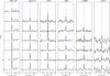 |
Fig. 1 Lines of C6H observed in this work toward six cold, dense clouds using the Yebes 40 m telescope. See the line parameters in Table A.1. |
3 Physical parameters of the sources
The interstellar clouds where the molecular anions have been detected comprise a total of 12, featuring cold, dense cores in different evolutionary stages, including: starless, prestellar, and protostellar (see Table 1). The classification as protostellar cores is evident in the cases of L1527 and L483, as the targeted positions are those of the infrared sources IRAS 04368+2557 and IRAS 18148−0440, respectively (Sakai et al. 2008; Agúndez et al. 2019). We also classified L1251A, L1172, and L1389 as protostellar sources based on the proximity of an infrared source (L1251AIRS3, CB17MMS, and IRAS21017+6742, respectively) to the positions targeted by Cordiner et al. (2013). The differentiation between starless and prestellar core is in some cases more ambiguous. In those cases we followed the criterion based on the N2D+/N2H+ column density ratio by Crapsi et al. (2005). In any case, for our purposes it is not very important whether a given core is starless or prestellar.
To study the abundance and excitation of molecular anions in these 12 interstellar sources through non-LTE calculations we need to know, which are the physical parameters of the clouds, mainly the gas kinetic temperature and the H2 volume density, as well as the emission size of anions and the linewidth. The adopted parameters are summarized in Table 1.
Given that C6H− has not been mapped in any interstellar cloud to date, it is not known whether the emission of molecular anions in each of the 12 sources is extended compared to the telescope beam sizes, which are in the range 21–67″ for the Yebes 40 m, IRAM 30 m, and GBT telescopes at the frequencies targeted for the observations of anions. Therefore one has to rely on maps of related species. In the case of TMC-1 CP we assume that anions are distributed in the sky as a circle with a diameter of 80″ based on the emission distribution of C6H mapped by Fossé et al. (2001). Recent maps carried out with the Yebes 40 m telescope (Cernicharo et al. 2023b) support the previous results of Fossé et al. (2001). For the remaining 11 sources, the emission distribution of C6H is not known and thus we assume that the emission of anions is extended with respect to the telescope beam. This assumption is supported by the extended nature of HC3N emission in the cases of L1495B, L1251A, L1512, L1172, L1389, and TMC-1 C, according to the maps presented by Cordiner et al. (2013), and of multiple molecular species, including C4H, in L1544, according to the maps reported by Spezzano et al. (2017).
The linewidth adopted for each source (see Table 1) was calculated as the arithmetic mean of the values derived for the lines of C6H− in the Q band for TMC-1 CP, Lupus-1A, L1527, L1495B, and L1544. In the case of L483, we adopted the value derived by Agúndez et al. (2019) from the analysis of all the lines in the 3 mm band. For L1521F, L1251A, L1512, L1172, and L1389, the adopted linewidths come from IRAM30m observations of CH3CCH in the 3 mm band (see Sect. 2.1). Finally, for TMC-1 C we adopted as linewidth that derived for HC3N by Cordiner et al. (2013).
The gas kinetic temperature was determined for some of the sources from the J = 5−4 and J = 6−5 rotational transitions of CH3CCH, which lie around 85.4 and 102.5 GHz, respectively. We have IRAM 30 m data of these lines for TMC-1 CP, Lupus-1A, L483, L1495B, and L1521F; while for L1527, we used the data obtained with the Nobeyama 45m telescope by Yoshida et al. (2019). Typically, the K = 0, 1, and 2 components are detected, thus allowing the use of the line intensity ratio between the K = 1 and K =2 components (belonging to the E symmetry species) to derive the gas kinetic temperature. Since transitions with ∆K ≠ 0 are radiatively forbidden, the relative populations of the K = 1 and K = 2 levels are controlled by collisions with H2 and are thus thermalized at the kinetic temperature of H2. We did not use the K = 0 component in this study because it belongs to a different symmetry species (i.e., A) and the interconversion process between A and E species is expected to be slow in cold, dense clouds; as a result, their relative populations may not necessarily reflect the gas kinetic temperature.
For TMC-1 CP, we derived kinetic temperatures of 8.8 ± 0.6 K and 9.0 ± 0.6 K from the J = 5−4 and J = 6−5 lines of CH3CCH, respectively. Similarly, using the i = 8−7 through J = 12−11 lines of CH3C4H, which lie in the Q band, we derive temperatures of 9.1 ± 0.7 K, 8.7 ± 0.6 K, 9.0 ± 0.6 K, 8.1 ± 0.7 K, and 9.1 ± 0.8 K, respectively. We thus adopted a gas kinetic temperature of 9 K, which is slightly lower than values derived in previous studies, 11.0 ± 1.0 K and 10.1 ± 0.9 K at two positions close to the cyanopolyyne peak using NH3 (Fehér et al. 2016) and 9.9 ± 1.5 K from CH2CCH (Agúndez et al. 2022). In Lupus-1A, we derived temperatures of 11.4 ± 1.7 K and 10.2 ± 1.1 K from the J = 5−4 and J = 6−5 lines of CH3 CCH, respectively. We thus adopted a gas kinetic temperature of 11 K, which is somewhat below the value of 14 ± 2 K derived in Agúndez et al. (2015) using the K = 0, 1, and 2 components of the J =5-4 transition of CH3CCH. In L1527, we derived 13.6 ± 2.5 K and 15.1 ± 2.4 K from the line parameters of CH3CCH J = 5−4 and J = 6−5 reported by Yoshida et al. (2019). We thus adopted a kinetic temperature of 14 K, which agrees perfectly with the value of 13.9 K derived by Sakai et al. (2008) using CH3CCH as well. The gas kinetic temperature in L483 has been estimated to be 10 K by Anglada et al. (1997), using NH3, while Agúndez et al. (2019) derive values of 10 K and 15 ± 2 K using either 13CO or CH3CCH. A new analysis of the CH3CCH data of Agúndez et al. (2019), in which the weak K = 3 components are neglected and only the K =1 and K = 2 components are used, gave kinetic temperatures of 11.5 ± 1.1 K and 12.6 ± 1.5 K, depending on whether the J =5−4 or J = 6−5 transition is used. We thus adopted a kinetic temperature of 12 K for L483. For L1495B we derive 9.1 ± 0.9 K and 9.2 ± 0.7 K from CH3CCH J = 5−4 and J = 6−5, and we thus adopted a kinetic temperature of 9 K. In L1521F, we adopted a gas kinetic temperature of 9 K as well, since the derived temperatures from CH3CCH J = 5−4 and J = 6−5 are 9.0 ± 0.7 K and 8.9 ± 0.9 K. This value agrees well with the temperature of 9.1 ± 1.0 K derived by Codella et al. (1997) using NH3. For the remaining cores, the gas kinetic temperatures were taken from the literature, as summarized in Table 1.
To estimate the volume density of H2, we used the 13C isotopologues of HC3N (when the data were available). We obtained Yebes 40 m data of the J = 4−3 and J =5−4 lines of H13CCCN, HC13CCN, and HCC13CN for TMC-1 CP, Lupus-1A, L1527, and L483. Data for one or various lines of these three isotopologues in the 3 mm band are also available from the IRAM 30 m telescope (see Sect. 2.1) or from the Nobeyama 45 telescope (for L1527; see Yoshida et al. 2019). Using the 13C isotopologues of HC3N turned out to constrain much better the H2 density that using the main isotopologue because one gets rid of optical depth effects. We carried out non-LTE calculations under the large velocity gradient (LVG) formalism adopting the gas kinetic temperature and linewidth given in Table 1 and varying the column density of the 13C isotopologue of HC3N and the H2 volume density. As collision rate coefficients we used those calculated by Faure et al. (2016) for HC3N with ortho and para H2, where we adopted a low ortho-to-para ratio of H2 of 10−3, which is theoretically expected for cold dark clouds (e.g., Flower et al. 2006). The exact value of the ortho-to-para ratio of H2 is not very important as long as the para form is well in excess of the ortho form, so that collisions with para H2 dominate. The best estimates for the column density of the 13C isotopologue of HC3N and the volume density of H2 are found by minimizing χ2, which is defined as:
![Mathematical equation: $ {\chi ^2} = {\sum\limits_{i = 1}^{{N_l}} {\left[ {{{\left( {{I_{{\rm{calc}}}} - {I_{{\rm{obs}}}}} \right)} \over \sigma }} \right]} ^2}, $](/articles/aa/full_html/2023/09/aa47077-23/aa47077-23-eq2.png) (1)
(1)
where the sum extends over the Nl lines available, Icalc and Iobs are the calculated and observed velocity-integrated brightness temperatures, and σ are the uncertainties in Iobs, which include the error given by the Gaussian fit and the calibration error of 10%. To evaluate the goodness of the fit, we use the reduced χ2, which is defined as  , where
  is the minimum value of χ2 and p is the number of free parameters. Typically, a value of
  indicates a good quality of the fit. In this case we have p = 2 because there are two free parameters, the column density of the 13C isotopologue of HC3N and the H2 volume density. Errors in these two parameters are given as 1 σ, where for p = 2, the 1 σ level (68% confidence) corresponds to χ2+2.3. The same statistical analysis is adopted in Sect. 5 when studying molecular anions and their neutral counterparts through the LVG method. In some cases in which the number of lines is small or the H2 density is poorly constrained, the H2 volume density is kept fixed. In those cases p = 1 and the 1 σ error (68% confidence) in the column density is given by, χ2+1.0.
In Fig. 4, we show the results for TMC-1 CP. In this starless core the H2 volume density is well constrained by the four available lines of the three 13C isotopologues of HC3N to a narrow range of (0.9−1.1) × 104 cm−3 with very low values of  . We adopt as H2 density in TMC-1 CP the arithmetic mean of the values derived for the three isotopologues, that is, 1.0 × 104 cm−3 (see Table 1). Similar calculations allow to derive H2 volume densities of 1.8 × 104 cm−3 for Lupus-1A, 5.6 × 104 cm−3 for L483, and a lower limit of 105 cm−3 for L1527 (see Table 1). The value for L483 is of the same order than those derived in the literature, 3.4 × 104 cm−3 from the model of Jørgensen et al. (2002) and 3 × 104 cm−3, from either NH3 (Anglada et al. 1997) or CH3OH (Agúndez et al. 2019). For L1495B, we could only retrieve data for one of the 13C isotopologues of HC3N, HCC13CN, from which we derive a H2 density of 1.6 × 104 cm−3 (see Table 1). In the case of L1521F, 13C isotopologues of HC3N were not available and thus we used lines of HCCNC, adopting the collision rate coefficients calculated by Bop et al. (2021), to derive a rough estimate of the H2 volume density of 1 × 104 cm−3 (see Table 1). Higher H2 densities, in the range (1–5) × 105 cm−3, are derived for L1521F from N2H+ and N2D+ (Crapsi et al. 2005), probably because these molecules trace the innermost dense regions depleted in CO.
For the remaining sources we adopted H2 volume densities from the literature (see Table 1). For L1544 we adopted a value of 2 × 104 cm−3 from the analysis of SO and SO2 lines by Vastel et al. (2018). This H2 density is in agreement with the range of values, (1.5–4.0) × 104 cm−3, found by Bop et al. (2022) in their excitation analysis of HCCNC and HNC3. We note that H2 volume densities toward the dust peak are larger than 106 cm−3. However, as shown by Spezzano et al. (2017), the emission of C4H probes the outer shells and thus a density of a few 104 cm−3 is appropriate for our calculations toward the CH3OH peak. In the cases of L1251A, L1512, L1172, L1389, and TMC-1 C, we adopted the H2 densities from the analysis of HC3N lines by Cordiner et al. (2013). The reliability of the H2 volume densities derived by these authors is supported by the fact that the densities they derive for TMC-1 CP and L1495B, 1.0 × 104 cm−3, and 1.1 × 104 cm−3, respectively, are close to the values determined in this study from 13C isotopologues of HC3N (see Table 1).
In spite of the different evolutionary status of the 12 anion-containing clouds, the gas kinetic temperatures, and H2 volume densities at the scales proven by the Yebes 40 m, IRAM 30 m, and GBT telescopes are not that different. Gas temperatures are restricted to the very narrow range 9–14 K, while H2 densities are in the range (1.0–7.5) × 104 cm−3, at the exception of L1527 which has an estimated density in excess of 105 cm−3 (see Table 1).
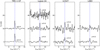 |
Fig. 2 Lines of C4N− observed in this work toward TMC-1 CP, Lupus-1A, L1527, and L483 using the Yebes 40 m and IRAM 30 m telescopes. See the line parameters in Table A.1. |
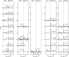 |
Fig. 3 Lines of C8N− observed toward TMC-1 CP and lines of the nitrile anions C3N− and C5N− observed toward TMC-1 CP and Lupus-1A using the Yebes 40 m and IRAM 30 m telescopes. See the line parameters in Table A.1. |
Source parameters.
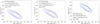 |
Fig. 4 χ2 as afunction of H2 volume density and column density of each of the three 13C isotopologues of HC3N in TMC-1 CP. Contours correspond to 1, 2, and 3 σ levels. The three maps have the same scale in the x and y axes to facilitate the comparison. The column density of HCC13CN is clearly higher than those of H13CCCN and HC13CCN. The volume density of H2 is constrained to a very narrow range, (0.9–1.1) × 104 cm−3, by the three 13C isotopologues of HC3N. |
4 Excitation of anions: General considerations
We could expect that given the large dipole moments of molecular anions, reaching as high as 10.4 D in the case of C8H− (Blanksby et al. 2001), rotational levels would be populated out of thermodynamic equilibrium in cold dark clouds. This is not always the case, as we go on to show here. To get insights into the excitation of negative molecular ions in interstellar clouds, we ran non-LTE calculations under the LVG formalism adopting typical parameters of cold dark clouds, namely, a gas kinetic temperature of 10 K, a column density of 1011 cm−2 (of the order of the values typically derived for anions in cold dark clouds; see references in Sect. 2.2), and a linewidth of 0.5 km s−1 (see Table 1). We varied the volume density of H2 between 103 and 106 cm−3. The sets of rate coefficients for inelastic collisions with H2 adopted are summarized in Table 2. In cases where only collisions with He were available, we scaled the rate coefficients by multiplying them by the square root of the ratio of the reduced masses of the H2 and He colliding systems. When inelastic collisions for ortho and para H2 were available, we adopted a ortho-to-para ratio of H2 of 10−3.
In Fig. 5, we show the calculated excitation temperatures (Tex) of lines of molecular anions as a function of the quantum number J of the upper level and the H2 volume density. The different panels correspond to different anions and show the regimes in which lines are either thermalized (Tex ~ 10 K) of subthermally excited (Tex < 10 K). To interpret these results, it is useful to think in terms of the critical density, which for a given rotational level can be evaluated as the ratio of the de-excitation rates due to spontaneous emission and due to inelastic collisions (e.g., Lara-Moreno et al. 2019). Collision rate coefficients for transitions with ∆J = −1 or −2, which are usually the most efficient, are on the order of 10−10 cm3 s−1 at a temperature of 10 K for the anions for which calculations have been carried out (see Table 2). The Einstein coefficient for spontaneous emission depends linearly on the square of the dipole moment and the cube of the frequency. Therefore, the critical density (and thus the degree of departure from LTE) is very different depending on the dipole moment of the anion and on the frequency of the transition. Regarding the dependence of the critical density on the dipole moment, C2H− and CN− have a similar weight, thus their low-J lines (the ones that are observable for cold clouds) have similar frequencies. However, these two anions have quite different dipole moments, 3.1 and 0.65 Debye, respectively (Brünken et al. 2007b; Botschwina et al. 1995), which make them show a different excitation pattern. As seen in Fig. 5, the low-J lines of CN− are in LTE at densities above 105 cm−3, while those of C2H− require much higher H2 densities to verifiably be in LTE. With respect to the dependence of the critical density with frequency, as we move along the series of increasing weight C2H− → C4H− → C6H− or CN− → C3N− → C5N− (see Fig. 5), the most favorable lines for detection in cold clouds (those with upper level energies around 10 K) shift to lower frequencies, which cause the Einstein coefficients (and thus the critical densities) to decrease. That is to say, the lines of anions targeted by radiotelescopes are more likely to be thermalized for heavy anions than for light ones (see the higher degree of thermalization when moving from lighter to heavier anions in Fig. 5).
The volume densities of H2 in cold dark clouds are typically in the range of 104-105 cm−3 (see Table 1). Therefore, if C2H− is detected in a cold dark cloud at some point in the future, the most favorable line for detection, namely, J = 1−0, would most likely be subthermally excited, making it necessary to use the collision rate coefficients to derive a precise abundance. In the case of a potential future detection of CN− in a cold interstellar cloud, the J = 1−0 line would be in LTE only if the H2 density of the cloud is ≥ 105 cm−3 and out of LTE for lower densities (see Fig. 5). The medium-sized anions C4H− and C3N− are predicted to have their Q band lines more or less close to LTE depending on whether the H2 density is closer to 105 or to 104 cm−3, while the lines in the 3 mm band are likely to be subthermally excited unless the H2 density is above 105 cm−3 (see Fig. 5). For the heavier anions, C6H− and C5N−, the lines in the K band are predicted to be thermalized at the gas kinetic temperature, while those in the Q band may or may not be thermalized depending on the H2 density (see Fig. 5). Comparatively, the Q band lines of C5N− are more easily thermalized than those of C6H− because C5N− has a smaller dipole moment than C6H−. We note that the results concerning C5N− have to be taken with caution because we used the collision rate coefficients calculated for C6H− in the absence of specific collision data for C5N− (see Table 2). We carried out similar calculations for C8H−, C10H−, and C7N− (not shown) using the collision rate coefficients of C6H−. We find that the lines in a given spectral range deviate more from thermalization as the size of the anion increases. In the K band, the lines of C6H− and C5N− are thermalized, while those of C10H− become subthermally excited at low densities, namely, around 104 cm−3. In the Q band, the deviation from thermalization is even more marked for these large anions.
In summary, non-LTE calculations are particularly important in deriving accurate abundances for anions when just one or two lines are detected, and these lie in a regime of subthermal excitation, as indicated in Fig. 5. This becomes critical, in order of decreasing importance, for C2H−, CN−, C4H−, C3N−, C6H−, C8H−, and C5N− (for the latter three: only if observed at frequencies above 30 GHz). The drawback is that the H2 volume density must be known with a good precision when we are aiming to determine the anion column density accurately based on only one or two lines.
In the case of the neutral counterparts of molecular anions, collision rate coefficients have been calculated for C6H and C3N, with He as a collider (Walker et al. 2018; Lara-Moreno et al. 2021). We thus carried out LVG calculations similar to those presented before for anions. In this case, we adopted a higher column density of 1012 cm−2, in line with typical values in cold dark clouds (see references in Sect. 2.2). The results are shown in Fig. 6. It can be seen that in the case of C3N, the excitation pattern is similar to that of the corresponding anion, C3N−, shown in Fig. 5. The thermalization of C3N occurs at densities somewhat higher compared to C3N−, mainly because the collision rate coefficients calculated for C3N with He (Lara-Moreno et al. 2021) are smaller than those computed for C3N− with para H2 (Lara-Moreno et al. 2019). We note that this conclusion may change if the collision rate coefficients of C3N with H2 are significantly larger than the factor of 1.39 due to the change in the reduced mass when changing He by H2. However, in the case of C6H, the excitation behavior is very different to that of C6H− (compare C6H− in Fig. 5 with C6H in Fig. 6). The rotational levels of the radical are much more subthermally excited than those of the corresponding anion, with a difference in the critical density of about a factor of 30. This is a consequence of the much smaller collision rate coefficients calculated for C6H with He (Walker et al. 2018) compared to those calculated for C6H− with para H2 (Walker et al. 2017), a difference that is well beyond the factor of 1.40 due to the change in the reduced mass when changing He by H2.
Collision rate coefficients used in this study.
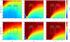 |
Fig. 5 Excitation temperature (color-coded map) as a function of quantum number of upper level (x-axis) and H2 volume density (y-axis) for six negative molecular anions as obtained from LVG calculations adopting a gas kinetic temperature of 10 K, a column density of 1011 cm−2, and a linewidth of 0.5 km s−1. The references for the dipole moments are Brünken et al. (2007b) for C2H−, Botschwina (2000) for C4H−, Blanksby et al. (2001) for C6H−, Botschwina et al. (1995) for CN−, Thaddeus et al. (2008) and Kołos et al. (2008) for C3N−, and Botschwina & Oswald (2008) for C5N−. For reference, the white dotted vertical line indicates the J level at which the energy is 10 K. The microwave and mm spectral regions observable with radiotelescopes are indicated. The small dark blue regions in the bottom-left corner of the C4H−, C6H−, and C3N− panels correspond to negative excitation temperatures. |
5 Anion abundances
We evaluated the column densities of molecular anions and their corresponding neutral counterparts in the 12 sources studied here by carrying out LVG calculations (similar to those described in Sect. 3) for the 13C isotopologues of HC3N. We used the collision rate coefficients given in Table 2. Gas kinetic temperatures and linewidths were fixed to the values given in Table 1, while the ortho-to-para ratio of H2, when needed, was fixed to 10−3, and both the column density of the species under study and the H2 volume density were varied. The best estimates for these two parameters were found by minimization of χ2 (see Sect. 3). In addition, we constructed rotation diagrams to evaluate the rotational temperature (and thus the level of departure from LTE) and to have an independent estimate of the column density.
The LVG method should provide a more accurate determination of the column density than the rotation diagram, as long as the collision rate coefficients with para H2 and the gas kinetic temperature are accurately known. If an independent determination of the H2 volume density is available from some density tracer (in our case the 13C isotopologues of HC3N are used in several sources), a good agreement between the values of n(H2) obtained from the species under study and from the density tracer supports the reliability of the LVG analysis. We note that densities do not need to be similar if the species studied and the density tracer are distributed over different regions, although in our case, we expected similar distributions for HC3N, molecular anions and their neutral counterparts, as long as all them are carbon chains.
A low value of  , typically ≲ 1, is also indicative of the goodness of the LVG analysis. If the quality of the LVG analysis is not satisfactory or the collision rate coefficients are not accurate, a rotation diagram may still provide a good estimate of the column density if the number of detected lines is high enough and they span a wide range of upper level energies. Therefore, a high number of detected lines makes it likely to end up with a correct determination of the column density. On the other hand, if only one or two lines are detected, the accuracy with which the column density can be determined relies heavily on whether the H2 volume density (in the case of an LVG calculation) or the rotational temperature (in the case of the rotation diagram) are known with some confidence.
In Table 3, we present the results from the LVG analysis and the rotation diagram for all molecular anions detected in cold dark clouds and for the corresponding neutral counterparts. We also compare the column densities derived with values from the literature, when available. In general, the column densities derived through the rotation diagram agree within a 50% margin of error with those derived by the LVG analysis. The sole exceptions are C8H in TMC-1 CP and C6H in TMC-1 C. In the former case, the lack of specific collision rate coefficients for C8H probably introduces an uncertainty in the determination of the column density. In the case of C6H in TMC-1 C, the suspected problem in the collision rate coefficients used for C6H (see below) is probably causing the overly large column density derived by the LVG method.
We go on to discuss the excitation and abundance analyses carried out for negative ions. For the anions detected in TMC-1 CP through more than two lines, namely, C6H−, C8H−, C3N−, and C5N−, the quality of the LVG analysis is good (in Fig. 7, we show the case of C3N−). First, the number of lines available is sufficiently high and they cover a wide range of upper level energies. Second, the values of  are ≲ 1. And third, the H2 densities derived are on the same order (within a factor of two) of that obtained through 13C isotopologues of HC3N. The rotational temperatures derived by the rotation diagram indicate subthermal excitation, which is consistent with the H2 densities derived and the excitation analysis presented in Sect. 4. We note that the column densities derived by the rotation diagram are systematically higher, by ~50%, compared to those derived through the LVG analysis. These differences are due to the breakdown of various assumptions made in the frame of the rotation diagram method, mainly the assumption of a uniform excitation temperature across all transitions and the validity of the Rayleigh-Jeans limit. Only the assumption that exp(hv/kTex) − 1 = hν/kTex, implicitly made by the rotation diagram method in the Rayleigh-Jeans limit, already implies errors of 10–20% in the determination of the column density for these anions. We therefore adopt, as the preferred values for the column densities, the ones derived through the LVG method and we assigned an uncertainty of 15%, which is the typical statistical error in the determination of the column density by the LVG analysis. The recommended values are given in Table 4. Based on the same arguments, we conclude that the LVG analysis is satisfactory for C6H− and C5N− in Lupus-1A, C6H− and C4H− in L1527, and C6H− in L483; thus, we adopted the column densities derived by the LVG method with the same estimated uncertainty of 15% (see Table 4). In other cases, the LVG analysis is less reliable due to a variety of reasons: only one or two lines are available (C4H− in TMC-1 CP, C8H− and C3N− in Lupus-1A, C4H− in L483, and C6H− in the clouds L1521F, L1251A, L1512, L1172, L1389, and TMC-1 C), the parameter
  is well above unity (C4H− in Lupus-1A) or the column density has a sizable error (C6H− in L1495B and L1544). In those cases, we adopted the column densities derived by the LVG method, but assigned a higher uncertainty, namely, of 30% (specific values are given in Table 4).
In order to derive anion-to-neutral abundance ratios, we applied the same analysis carried out for the anions to the corresponding neutral counterparts. We first focused on the radical C6H. There is one striking issue in the LVG analysis carried out for this species: the H2 volume densities derived through C6H are systematically higher, by one to two orders of magnitude, than those derived through the 13C isotopologues of HC3N (see Fig. 8). This fact, together with the previous marked difference in the excitation pattern compared to that of C6H− discussed in Sect. 4, suggests that the collision coefficients adopted for C6H, which are based on the C6H − He system studied by Walker et al. (2018), are too small. A further problem when using the collision coefficients of Walker et al. (2018) is that the line intensities from the 2Π1/2 state, which in TMC-1 CP are around 100 times smaller than those of the 2Π3/2 state, are overestimated by a factor of ~10. All these issues indicate that it is worth to undertake calculations of the collision rate coefficients of C6H with H2. The suspected problem in the collision rate coefficients of C6H make us to adopt a conservative uncertainty of 30% in the column densities derived. Moreover, in those sources in which C6H is observed through just a few lines (L1521F, L1251A, L1512, L1172, L1389, and TMC-1 C), we needed to fix the H2 density to the values derived through other density tracers (see Table 1). Also, given the marked difference between the H2 densities derived through C6H and other density tracers, it is likely that the C6H column densities derived by the LVG method are unreliable. In these cases, we thus adopted, as preferred C6H column densities, those obtained from the rotation diagram (see Table 4). For the other neutral radicals, we adopted the column densities derived by the LVG method with an estimated uncertainty of 15% when the LVG analysis was satisfactory (C3N and C5N in TMC-1 CP, C4H, C3N, and C5N in Lupus-1A, and C4H in L1527) and a higher uncertainty of 30% otherwise (C4H and C8H in TMC-1 CP, C8H in Lupus-1A, and C4H in L483).
The recommended column densities for molecular anions and their neutral counterparts, and the corresponding anion-to-neutral ratios, are given in Table 4. Since the lines of a given anion and its corresponding neutral counterpart where in most cases observed simultaneously, we expect the error due to calibration to cancel when computing anion-to-neutral ratios. We therefore subtracted the 10% error due to calibration in the column densities when computing errors in the anion-to-neutral ratios. In general, the recommended anion-to-neutral abundance ratios agree within 50% with the values reported in the literature, when available. Higher differences, of up to a factor of 2, are found for C6H− in L1527 and L1495B and for C5N− in TMC-1 CP. The most drastic differences are found for the C4H−/C4H abundance ratio, for which we derive values much higher than those reported in the literature. The differences are largely due to the fact that we have adopted a revised value of the dipole moment of C4H (2.10 D; Oyama et al. 2020), which is significantly higher than the value of 0.87 D calculated by Woon (1995) and adopted in previous studies. This fact makes the column densities of C4H to be revised downward by a factor of ~6 and, consequently, the C4H−/C4H ratios are also revised upward by the same factor.
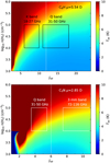 |
Fig. 6 Same as Fig. 5 but for the radicals C6H and C3N adopting in this case a column density of 1012 cm−2. The references for the dipole moments are Woon (1995) for C6H and McCarthy et al. (1995) for C3N. |
Results from LVG and rotation diagram analyses.
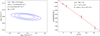 |
Fig. 7 Excitation and abundance analysis for C3N− in TMC-1 CP. Left panel shows χ2 as a function of the H2 volume density and the column density of C3N−, where the contours correspond to 1, 2, and 3 σ levels. Right panel shows the rotation diagram. |
Recommended column densities and anion-to-neutral abundance ratios.
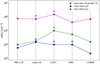 |
Fig. 8 Volume density of H2 in various cold dark clouds determined through LVG calculations using different tracers. Green points correspond to densities derived from 13C isotopologues of HC3N (see values in Table 1), while blue and magenta points correspond to densities obtained from the anion C6H− and the radical C6H, respectively (see values in Table 3). H2 densities derived through C6H− are close to those derived by 13C isotopologues of HC3N, while H2 densities derived through C6H are systematically higher by factors of 10-50. |
6 Discussion
Having access to a rather complete observational picture of negative ions in the interstellar medium, as summarized in Table 4, it is interesting to examine the lessons that can be drawn on this basis. There are at least two interesting aspects to discuss. First, we ask how the anion-to-neutral abundance ratio behave from one source to another, and whether the observed variations can be related to some property of the cloud. Second, within a given source, we ask how the anion-to-neutral abundance ratio vary for the different anions, and whether this can be related to the formation mechanism of anions.
Regarding the first point, since C6H− is the most widely observed anion, it is very convenient to focus on it to investigate the source-to-source behavior of negative ions. The detection of C6H− in L1527 and the higher C6H−/C6H ratio derived in that source compared to that in TMC-1 CP led Sakai et al. (2007) to suggest that this was a consequence of the higher H2 density in L1527 compared to TMC-1 CP. This point was later on revisited by Cordiner et al. (2013), with a larger number of sources detected in C6H−. These authors found a trend in which the C6H−/C6H ratio increases with increasing H2 density and further argued that this ratio increases as the cloud evolves from quiescent to star-forming, with ratios below 3% in quiescent sources and above that level in star-forming ones.
There are theoretical grounds that support a relationship between the C6H−/C6H ratio and the H2 density. Assuming that the formation of anions is dominated by radiative electron attachment to the neutral counterpart and that they are mostly destroyed through reaction with H atoms, as expected for the conditions of cold, dense clouds (Flower et al. 2007), it can be easily shown that at steady state, the anion-to-neutral abundance ratio is proportional to the abundance ratio between electrons and H atoms, which, in turn, is proportional to the square root of the H2 volume density (e.g., Flower et al. 2007). That is to say,
 (2)
(2)
In Fig. 9, we plot the observed C6H−/C6H ratio as a function of the H2 density for the 12 clouds where this anion has been detected. This is an extended and updated version of Fig. 5 of Cordiner et al. (2013), where we superimpose the theoretical trend expected according to Eq. (2). In general terms, the situation depicted by Fig. 9 is not that different from that found by Cordiner et al. (2013). The main difference concerns L1495B, for which we derive a higher C6H−/C6H ratio, 3.0% instead of 1.4%. Our value should be more accurate, given the larger number of lines used here. Apart from that, the C6H−/C6H ratio tends to be higher in those sources with higher H2 densities, which tend to be more evolved. This behavior is similar to that found by Cordiner et al. (2013). The data points in Fig. 9 seem to be consistent with the theoretical expectation. We however caution that there is substantial dispersion in the data points. Moreover, the uncertainties in the anion-to-neutral ratios, together with those affecting the H2 densities (not shown), make it difficult to end up with a solid conclusion on whether or not observations follow the theoretical expectations. If we restrict our sample to the five best-characterized sources (TMC-1 CP, Lupus-1A, L1527, L483, and L1495B), with all them observed in C6H− through four or more lines and studied in the H2 density in a coherent way, then the picture is such that all sources, regardless of its H2 density, have similar C6H−/C6H ratios, at the exception of L1527, which remains the only data point supporting the theoretical relation between anion-to-neutral ratio and H2 density. It is also worth noting that when looking at C4H−, L1527 shows also an enhanced anion-to-neutral ratio compared to TMC-1 CP, Lupus-1A, and L483. Further detections of C6H− in sources with high H2 densities, preferably above 105 cm−3, should help to shed light on the suspected relation between anion-to-neutral ratio and H2 density. This however may not be easy because chemical models predict that, although the C6H−/C6H ratio increases with increasing H2 density, an increase in the density also brings a decrease in the column density of both C6H and C6H− (Cordiner & Charnley 2012).
The second aspect that is worth to discuss is the variation of the anion-to-neutral ratio for different anions within a given source. Unlike the former source-to-source case, where variations were small (a factor of two at most), here anion-to-neutral ratios vary by orders of magnitude, i.e., well above uncertainties. Figure 10 summarizes the observational situation of interstellar anions in terms of abundances relative to their neutral counterpart. The variation of the anion-to-neutral ratios across different anions is best appreciated in TMC-1 CP and Lupus-1A, which stand out as the two most prolific sources of interstellar anions. The lowest anion-to-neutral ratio is reached by far for C4H−, while the highest values are found for C5N− and C8H−. We caution that the C5N−/C5N ratio could have been overestimated if the true dipole moment of C5N is a mixture between those of the 2Σ and 2Π states, as discussed by Cernicharo et al. (2008), in a case similar to that studied for C4H by Oyama et al. (2020). For the large anion C7N−, the anion-to-neutral ratio is not known in TMC-1 CP, but it is probably large, as suggested by the detection of the lines of the anion and the non-detection of the lines of the neutral (Cernicharo et al. 2023a). In the case of the even larger anion C10H−, the anion is found to be even more abundant than the neutral in TMC-1 CP by a factor of two, although this result has probably an important uncertainty since the detection is done by line stack (Remijan et al. 2023). Moreover, it is yet to be confirmed that the species identified is C10H− and not C9N− (Pardo et al. 2023). In any case, a solid conclusion from the TMC-1 CP and Lupus-1A data shown in Fig. 10 is that when we are looking at either the hydrocarbon series of anions or at the nitrile series, the anion-to-neutral ratio clearly increases with increasing size. The most straightforward interpretation of this behavior is related to the formation mechanism originally proposed by Herbst (1981), which relies on the radiative electron attachment (REA) to the neutral counterpart and for which the rate coefficient is predicted to increase markedly with increasing molecular size.
If electron attachment is the dominant formation mechanism of anions and destruction rates are similar for all anions, we expect the anion-to-neutral abundance ratio to be proportional to the rate coefficient of radiative electron attachment; namely,
 (3)
(3)
where A− and A are the anion and its corresponding neutral counterpart, respectively, and kREA is the rate coefficient for radiative electron attachment to A.
To get insight into this relation we plot in Fig. 10 the rate coefficients calculated for the reactions of electron attachment forming the different anions on a scale designed on purpose to visualize if observed anion-to-neutral ratios scale with calculated electron attachment rates. We arbitrarily choose C6H− as the reference for the discussion. If we first focus on the largest anion C8H−, we see that the C8H−/C8H ratios are systematically higher, by a factor of 2–3, than the C6H−/C6H ones; while Herbst & Osamura (2008) calculated identical electron attachment rates for C6H and C8H. Similarly, the C5N−/C5N ratios are higher, by a factor of 6–8 than the C6H−/C6H ratios, while the electron attachment rate calculated for C5N is twice that computed for C6H in the theoretical scenario of Herbst & Osamura (2008). That is to say, for the large anions C8H− and C5N−, there is a deviation by a factor of 2–4 from the theoretical expectation given by Eq. (3). This deviation is small given the various sources of uncertainties in both the observed anion-to-neutral ratio (mainly due to uncertainties in the dipole moments) and the calculated electron attachment rate coefficient. The situation is different for the medium size anions C4H− and C3N−. In the case of C4H−, anion-to-neutral ratios are ~100 times lower than for C6H−, while the electron attachment rate calculated for C4H is just about six times lower than that computed for C6H. The deviation from Eq. (3) of a factor ~20 (which is significant) is most likely due to the electron attachment rate calculated for C4H by Herbst & Osamura (2008) being too large. In the case of C3N−, the observed anion-to-neutral ratios are four to six times lower than those derived for C6H−, while the electron attachment rate calculated by Petrie & Herbst (1997) for C3N is 300 times lower than that computed for C6H by Herbst & Osamura (2008). Here, the deviation is as large as two orders of magnitude and it is probably caused by the too low electron attachment rate calculated for C3N. In summary, calculated electron attachment rates are consistent with observed anion-to-neutral ratios for the large species but not for the medium-sized species C4H and C3N; in those cases, the calculated rates are too large by a factor of ~20 and too small by a factor of ~ 100, respectively.
Of course, the above conclusion holds in the scenario of anion formation dominated by electron attachment and similar destruction rates for all anions, which may not be strictly valid. For example, it has been argued (Douguet et al. 2015; Khamesian et al. 2016; Forer et al. 2023) that the process of radiative electron attachment is much less efficient than has been calculated by Herbst & Osamura (2008), with rate coefficients that are too small to sustain the formation of anions in interstellar space. Millar et al. (2017) discussed this point, making the difference between direct and indirect radiative electron attachment, where, for long carbon chains, the direct process would be slow, corresponding to the rates calculated by Khamesian et al. (2016). Meanwhile, the indirect process could be fast if a long-lived superexcited anion is formed, which has some experimental support. Millar et al. (2017) conclude that there are enough grounds to support rapid electron attachment to large carbon chains, as calculated by Herbst & Osamura (2008). The formation mechanism of anions through electron attachment is very selective for large species and thus holds the advantage of naturally explaining the marked dependence of anion-to-neutral ratios with molecular size illustrated in Fig. 10, something that would be difficult to explain through other formation mechanism. Indeed, mechanisms such as dissociative electron attachment to metastable isomers such as HNC3 and H2C6 (Petrie & Herbst 1997; Sakai et al. 2007) or reactions of H− with polyynes and cyanopolyynes (Vuitton et al. 2009; Martínez et al. 2010; Khamesian et al. 2016; Gianturco et al. 2016; Murakami et al. 2022) could contribute to some extent but are unlikely to control the formation of anions, since they can hardly explain why large anions are far more abundant than small ones.
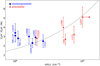 |
Fig. 9 Anion-to-neutral ratio C6H−/C6H (see values in Table 4) as a function of H2 volume density. We do not give the errors in the H2 densities because this parameter is not derived in a coherent way for all sources (see Table 1). The dotted line represents the trend expected according to theory (see text). |
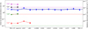 |
Fig. 10 Observed anion-to-neutral abundance ratios (referred to the left y axis) in cold interstellar clouds where molecular anions have been detected to date. Values are given in Table 4. Referred to the right y axis and following the same color code we also plot as dotted horizontal lines the calculated rate coefficients at 300 K for the reaction of radiative electron attachment to the neutral counterpart. Adopted values are 1.1 × 10⁻⁸ cm3 s−1 for C4H, 6.2 × 10⁻⁸ cm3 s−1 for C6H and C8H (Herbst & Osamura 2008; they are shown slightly displaced for visualization purposes), 2.0 × 10⁻¹⁰ cm3 s−1 for C3N (Petrie & Herbst 1997; Harada & Herbst 2008), and 1.25 × 10⁻⁷ cm3 s−1 for C5N (Walsh et al. 2009). The scale of the right y axis is chosen to make the rate coefficient of electron attachment to C6H to coincide with the mean of C6H−/C6H ratios and to cover the same range in logarithmic scale than the left y axis, which allows to visualize any potential proportionality between anion-to-neutral ratio and radiative electron attachment rate. |
7 Conclusions
We report new detections of molecular anions in cold, dense clouds. We have also significantly expanded the number of lines through which negative ions are detected in interstellar clouds. The most prevalent anion remains C6H−, which has been seen in 12 interstellar clouds to date, while the rest of interstellar anions are observed in only between one and four sources.
In this study, we carried out excitation calculations that indicate subthermal excitation is common for the lines of interstellar anions observed with radiotelescopes, with the low-frequency lines of heavy anions being the easiest to thermalize. Important discrepancies between calculations and observations are found for the radical C6H, which suggest that the collision rate coefficients currently available for this species need to be revisited.
We analyzed all the observational data acquired here and in previous studies through non-LTE LVG calculations and rotation diagrams to constrain the column density of each anion in each source. Differences in the anion-to-neutral abundance ratios with respect to literature values are small – less than 50% overall and even going up to a factor of 2 for a few cases. The greatest difference is found for the C4H−/C4H ratio, which is shifted upward with respect to previous values due to the adoption of a higher dipole moment for the radical C4H.
The observational picture of interstellar anions brought by this study demonstrates two interesting results. On the one side, the C6H−/C6H ratio seems to be higher in clouds with a higher H2 density, which is usually associated with a later evolutionary status of the cloud (although error bars make it difficult to clearly distinguish this trend). On the other hand, there is a very marked dependence of the anion-to-neutral ratio with the size of the anion, which is in line with the formation scenario involving radiative electron attachment; still, the theory must still be revised to account for medium-sized species such as C4H and C3N.
Acknowledgements
We acknowledge funding support from Spanish Ministerio de Ciencia e Innovación through grants PID2019-106110GB-I00, PID2019-107115GB-C21, and PID2019-106235GB-I00.
Appendix A Supplementary table
Observed line parameters of molecular anions in interstellar clouds.
Observed velocity-integrated line intensities of neutral counterparts of molecular anions in interstellar clouds.
a Unless otherwise stated, the intensity scale is antenna temperature ( ). It can be converted to main beam brightness temperature (Tmb) by dividing by Beff/Feff (see caption of Table A.1. The error in
  includes the contributions from the Gaussian fit and from calibration (assumed to be 10%). b Intensity scale is Tmb. c Intensity distributed equally among the two fine components. d Marginal detection.
References
- Agúndez, M., Cernicharo, J., Guélin, M., et al. 2008, A&A, 478, L19 [NASA ADS] [CrossRef] [EDP Sciences] [Google Scholar]
- Agúndez, M., Cernicharo, J., Guélin, M., et al. 2010, A&A, 517, A2 [NASA ADS] [CrossRef] [EDP Sciences] [Google Scholar]
- Agúndez, M., Cernicharo, J., & Guélin, M. 2015, A&A, 577, A5 [Google Scholar]
- Agúndez, M., Marcelino, N., Cernicharo, J., et al. 2019, A&A, 625, A147 [NASA ADS] [CrossRef] [EDP Sciences] [Google Scholar]
- Agúndez, M., Marcelino, N., Cabezas, C., et al. 2022, A&A, 657, A96 [NASA ADS] [CrossRef] [EDP Sciences] [Google Scholar]
- Agúndez, M., Roncero, O., Marcelino, N., et al. 2023, A&A, 673, A24 [NASA ADS] [CrossRef] [EDP Sciences] [Google Scholar]
- Alexander, M. H. 1982, J. Chem. Phys., 76, 5974 [NASA ADS] [CrossRef] [Google Scholar]
- Alexander, M. H., Smedley, J. E., & Corey, G. C. 1986, J. Chem. Phys., 84, 3049 [NASA ADS] [CrossRef] [Google Scholar]
- Anglada, G., Sepúlveda, I., & Gómez, J. F. 1997, A&AS, 121, 255 [NASA ADS] [CrossRef] [EDP Sciences] [Google Scholar]
- Bacmann, A., Lefloch, B., Ceccarelli, C., et al. 2002, A&A, 389, L6 [NASA ADS] [CrossRef] [EDP Sciences] [Google Scholar]
- Balança, C., Quintas-Sánchez, E., Dawes, R., et al. 2021, MNRAS, 508, 1148 [CrossRef] [Google Scholar]
- Biswas, R., Giri, K., González-Sánchez, L. et al. 2023, MNRAS, 522, 5775 [NASA ADS] [CrossRef] [Google Scholar]
- Blanksby, S. J., McAnoy, A. M., Dua, S., & Bowie, J. H. 2001, MNRAS, 328, 89 [NASA ADS] [CrossRef] [Google Scholar]
- Bop, C. T., Lique, F., Faure, A., et al. 2021, MNRAS, 501, 1911 [Google Scholar]
- Bop, C. T., Desrousseaux, B., & Lique, F. 2022, A&A, 662, A102 [NASA ADS] [CrossRef] [EDP Sciences] [Google Scholar]
- Botschwina, P. 2000, 55th Ohio Symposium on Molecular Spectroscopy, TC06 [Google Scholar]
- Botschwina, P. & Oswald, R. 2008, J. Chem. Phys., 129, 044305 [NASA ADS] [CrossRef] [Google Scholar]
- Botschwina, P., Seeger, S., Mladenovic, M., et al. 1995, Int. Rev. Phys. Chem., 14, 169 [NASA ADS] [CrossRef] [Google Scholar]
- Brünken, S., Gupta, H., Gottlieb, C. A., et al. 2007a, ApJ, 664, L43 [CrossRef] [Google Scholar]
- Brünken, S., Gottlieb, C. A., Gupta, H., et al. 2007b, A&A, 464, L33 [NASA ADS] [CrossRef] [EDP Sciences] [Google Scholar]
- Cabezas, C., Agúndez, M., Marcelino, N., et al. 2021, A&A, 654, A45 [NASA ADS] [CrossRef] [EDP Sciences] [Google Scholar]
- Cabezas, C., Agúndez, M., Marcelino, N., et al. 2022, A&A, 657, L4 [NASA ADS] [CrossRef] [EDP Sciences] [Google Scholar]
- Carelli, F., Satta, M., Grassi, T., & Gianturco, F. A. 2013, ApJ, 774, 97 [NASA ADS] [CrossRef] [Google Scholar]
- Cernicharo, J., Guélin, M., Agúndez, M., et al. 2007, A&A, 467, L37 [NASA ADS] [CrossRef] [EDP Sciences] [Google Scholar]
- Cernicharo, J., Guélin, M., Agúndez, M., et al. 2008, ApJ, 688, L83 [NASA ADS] [CrossRef] [Google Scholar]
- Cernicharo, J., Marcelino, N., Roueff, E., et al. 2012, ApJ, 759, L43 [NASA ADS] [CrossRef] [Google Scholar]
- Cernicharo, J., Marcelino, N., Pardo, J. R., et al. 2020, A&A, 641, L9 [NASA ADS] [CrossRef] [EDP Sciences] [Google Scholar]
- Cernicharo, J., Agúndez, M., Kaiser, R. I., et al. 2021, A&A, 652, A9 [Google Scholar]
- Cernicharo, J., Pardo, J. R., Cabezas, C., et al. 2023a, A&A, 670, A19 [NASA ADS] [CrossRef] [EDP Sciences] [Google Scholar]
- Cernicharo, J., Tercero, B., Marcelino, N., et al. 2023b, A&A, 674, L4 [NASA ADS] [CrossRef] [EDP Sciences] [Google Scholar]
- Codella, C., Welser, R., Henkel, C., et al. 1997, A&A, 324, 203 [NASA ADS] [Google Scholar]
- Cordiner, M. A., & Charnley, S. B. 2012, ApJ, 749, 120 [NASA ADS] [CrossRef] [Google Scholar]
- Cordiner, M. A., Charnley, S. B., Buckle, J. V., et al. 2011, ApJ, 730, L18 [NASA ADS] [CrossRef] [Google Scholar]
- Cordiner, M. A., Buckle, J. V., Wirström, E. S., et al. 2013, ApJ, 770, 48 [NASA ADS] [CrossRef] [Google Scholar]
- Crapsi, A., Caselli, P., Walmsley, C. M., et al. 2005, ApJ, 619, 379 [Google Scholar]
- Douguet, N., Fonseca dos Santos, S., Raoult, M., et al. 2015, J. Chem. Phys., 142, 234309 [NASA ADS] [CrossRef] [Google Scholar]
- Dumouchel, F., Spielfiedel, A., Senent, M. L., & Feautrier, N. 2012, Chem. Phys.Lett., 533, 6 [NASA ADS] [CrossRef] [Google Scholar]
- Dumouchel, F., Quintas-Sánchez, E., Balança, C., et al. 2023, J. Chem. Phys., 158, 164307 [NASA ADS] [CrossRef] [Google Scholar]
- Faure, A., Lique, A., & Wiesenfeld, L. 2016, MNRAS, 460, 2103 [NASA ADS] [CrossRef] [Google Scholar]
- Fehér, O., Tóth, L. V., Ward-Thompson, D., et al. 2016, A&A, 590, A75 [Google Scholar]
- Flower, D. R., Pineau des Forêts, G., & Walmsley, C. M. 2006, A&A, 449, 621 [NASA ADS] [CrossRef] [EDP Sciences] [Google Scholar]
- Flower, D. R., Pineau des Forêts, G., & Walmsley, C. M. 2007, A&A, 474, 923 [NASA ADS] [CrossRef] [EDP Sciences] [Google Scholar]
- Forer, J., Kokoouline, V., & Stoecklin, T. 2023, Phys. Rev. A, 107, 043117 [NASA ADS] [CrossRef] [Google Scholar]
- Fossé, D., Cernicharo, J., Gerin, M., & Cox, P. 2001, ApJ, 552, 168 [Google Scholar]
- Franz, J., Mant, B. P., González-Sánchez, L., et al. 2020, J. Chem. Phys., 152, 234303 [NASA ADS] [CrossRef] [Google Scholar]
- Frayer, D. T., Ghigo, F., & Maddalena, R. J. 2018, GBT Memo #301 [Google Scholar]
- Gianturco, F. A., Satta, M., Mendolicchio, M., et al. 2016, ApJ, 830, 2 [NASA ADS] [CrossRef] [Google Scholar]
- Gianturco, F. A., González-Sánchez, L., Mant, B. P., & Wester, R. 2019, J. Chem. Phys., 151, 144304 [NASA ADS] [CrossRef] [Google Scholar]
- González-Sánchez, L., Mant, B. P., Wester, R., & Gianturco, F. A. 2020, ApJ, 897, 75 [CrossRef] [Google Scholar]
- Gottlieb, C. A., Brünken, S., McCarthy, M. C., & Thaddeus, P. 2007, J. Chem. Phys., 126, 191101 [NASA ADS] [CrossRef] [Google Scholar]
- Gupta, H., Brünken, S., Tamassia, F., et al. 2007, ApJ, 655, L57 [NASA ADS] [CrossRef] [Google Scholar]
- Gupta, H., Gottlieb, C. A., McCarthy, M. C., & Thaddeus, P. 2009, ApJ, 691, 1494 [NASA ADS] [CrossRef] [Google Scholar]
- Harada, N., & Herbst, E. 2008, ApJ, 685, 272 [NASA ADS] [CrossRef] [Google Scholar]
- Herbst, E. 1981, Nature, 289, 656 [NASA ADS] [CrossRef] [Google Scholar]
- Herbst, E., & Osamura, Y. 2008, ApJ, 679, 1670 [NASA ADS] [CrossRef] [Google Scholar]
- Jiménez-Serra, I., Vasyunin, A. I., Caselli, P., et al. 2016, ApJ, 830, L6 [Google Scholar]
- Jørgensen, J. K., Schöier, F. L., & van Dishoeck, E. F. 2002, A&A, 389, 908 [CrossRef] [EDP Sciences] [Google Scholar]
- Khamesian, M., Douguet, N., Fonseca dos Santos, S., et al. 2016, Phys. Rev. Lett., 117, 123001 [NASA ADS] [CrossRef] [Google Scholar]
- Kłos, J., & Lique, F. 2011, MNRAS, 418, 271 [Google Scholar]
- Kołos, R., Gronowski, M., & Botschwina, P. 2008, J. Chem. Phys., 128, 154305 [CrossRef] [Google Scholar]
- Lara-Moreno, M., Stoecklin, T., & Halvick, P. 2017, MNRAS, 467, 4174 [NASA ADS] [CrossRef] [Google Scholar]
- Lara-Moreno, M., Stoecklin, T., & Halvick, P. 2019, MNRAS, 486, 414 [CrossRef] [Google Scholar]
- Lara-Moreno, M., Stoecklin, T., & Halvick, P. 2021, MNRAS, 507, 4086 [NASA ADS] [CrossRef] [Google Scholar]
- McCarthy, M. C., Gottlieb, C. A., Thaddeus, P., et al. 1995, J. Chem. Phys., 103, 7820 [NASA ADS] [CrossRef] [Google Scholar]
- McCarthy, M. C., Gottlieb, C. A., Gupta, H., & Thaddeus, P. 2006, ApJ, 652, L141 [NASA ADS] [CrossRef] [Google Scholar]
- Marcelino, N., Cernicharo, J., Agúndez, M., et al. 2007, ApJ, 665, L127 [Google Scholar]
- Martínez, O., Jr., Yang, Z., Demarais, N. J., et al. 2010, ApJ, 720, 173 [CrossRef] [Google Scholar]
- Millar, T. J., Walsh, C., & Field, T. A. 2017, Chem. Rev., 117, 1765 [CrossRef] [Google Scholar]
- Murakami, T., Iida, R., Hashimoto, Y., et al. 2022, J. Phys. Chem. A, 126, 9244 [NASA ADS] [CrossRef] [Google Scholar]
- Oyama, T., Ozaki, H., Sumiyoshi, Y., et al. 2020, ApJ, 890, 39 [NASA ADS] [CrossRef] [Google Scholar]
- Pardo, J. R., Cabezas, C., Agúndez, M., et al. 2023, A&A, 677, A55 [NASA ADS] [CrossRef] [EDP Sciences] [Google Scholar]
- Petrie, S., & Herbst, E. 1997, ApJ, 491, 210 [NASA ADS] [CrossRef] [Google Scholar]
- Punanova, A., Caselli, P., Feng, S., et al. 2018, ApJ, 855, 112 [NASA ADS] [CrossRef] [Google Scholar]
- Remijan, A. J., Hollis, J. M., Lovas, F. J., et al. 2007, ApJ, 664, L47 [NASA ADS] [CrossRef] [Google Scholar]
- Remijan, A., Scolati, H. N., Burkhardt, A. M., et al. 2023, ApJ, 944, L45 [NASA ADS] [CrossRef] [Google Scholar]
- Sakai, N., Sakai, T., Osamura, Y., & Yamamoto, S. 2007, ApJ, 667, L65 [NASA ADS] [CrossRef] [Google Scholar]
- Sakai, N., Sakai, T., Hirota, T., & Yamamoto, S. 2008, ApJ, 672, 371 [Google Scholar]
- Sakai, N., Shiino, T., Hirota, T., et al. 2010, ApJ, 718, L49 [NASA ADS] [CrossRef] [Google Scholar]
- Senent, M. L., Dayou, F., Dumouchel, F., et al. 2019, MNRAS, 486, 422 [NASA ADS] [CrossRef] [Google Scholar]
- Spezzano, S., Caselli, P., Bizzocchi, L., et al. 2017, A&A, 606, A82 [NASA ADS] [CrossRef] [EDP Sciences] [Google Scholar]
- Suzuki, H., Yamamoto, S., Ohishi, M., et al. 1992, ApJ, 392, 551 [Google Scholar]
- Tafalla, M., Myers, P. C., Caselli, P., et al. 2002, ApJ, 569, 815 [CrossRef] [Google Scholar]
- Tchakoua, T., Motapon, O., & Nsangou, M. 2018, J. Phys. B: At. Mol. Opt. Phys., 51, 045202 [NASA ADS] [CrossRef] [Google Scholar]
- Tercero, F., López-Pérez, J. A., Gallego, J. D., et al. 2021, A&A, 645, A37 [EDP Sciences] [Google Scholar]
- Thaddeus, P., Gottlieb, C. A., Gupta, H., et al. 2008, ApJ, 677, 1132 [NASA ADS] [CrossRef] [Google Scholar]
- Toumi, I., Yazidi, O., & Najar, F. 2021, RSC Adv., 11, 13579 [NASA ADS] [CrossRef] [Google Scholar]
- Vastel, C., Quénard, D., Le Gal, R., et al. 2018, MNRAS, 478, 5514 [Google Scholar]
- Visser, A. E., Richer, J. S., & Chandler, C. J. 2002, ApJ, 124, 2756 [CrossRef] [Google Scholar]
- Vuitton, V., Lavvas, P., Yelle, R. V., et al. 2009, Planet. Space Sci., 57, 1558 [NASA ADS] [CrossRef] [Google Scholar]
- Walker, K. M., Dumouchel, F., Lique, F., & Dawes, R. 2016, J. Chem. Phys., 145, 024314 [Google Scholar]
- Walker, K. M., Lique, F., Dumouchel, F., & Dawes, R. 2017, MNRAS, 466, 831 [Google Scholar]
- Walker, K. M., Lique, F., & Dawes, R. 2018, MNRAS, 473, 1407 [NASA ADS] [CrossRef] [Google Scholar]
- Walsh, C., Harada, N., Herbst, E., & Millar, T. J. 2009, ApJ, 700, 752 [NASA ADS] [CrossRef] [Google Scholar]
- Woon, D. E. 1995, Chem. Phys. Lett., 244, 45 [NASA ADS] [CrossRef] [Google Scholar]
- Yoshida, K., Sakai, N., Nishimura, Y., et al. 2019, PASJ, 71, S18 [NASA ADS] [CrossRef] [Google Scholar]
TMC-1 CP: αJ2000 = 4h41m41.9s and δJ2000 = +25°41′27.0″.
Lupus-1A: αJ2000 = 15h42m52.4s and δJ2000 =−34º07′53.5″.
L1495B: αJ2000 = 4h15m41.8s and δJ2000 = +28º47′46.0″.
L1544: αJ2000 = 5h4m18.0s and δJ2000 = +25º11′10.0″.
L1527: αJ2000 = 4h39m53.9s and δJ2000 = +26º03′11.0″.
L483: αJ2000 = 18h17m29.8s and δJ2000 =−1º39′38.3″.
All Tables
Observed velocity-integrated line intensities of neutral counterparts of molecular anions in interstellar clouds.
All Figures
|
Fig. 1 Lines of C6H observed in this work toward six cold, dense clouds using the Yebes 40 m telescope. See the line parameters in Table A.1. |
| In the text | |
|
Fig. 2 Lines of C4N− observed in this work toward TMC-1 CP, Lupus-1A, L1527, and L483 using the Yebes 40 m and IRAM 30 m telescopes. See the line parameters in Table A.1. |
| In the text | |
|
Fig. 3 Lines of C8N− observed toward TMC-1 CP and lines of the nitrile anions C3N− and C5N− observed toward TMC-1 CP and Lupus-1A using the Yebes 40 m and IRAM 30 m telescopes. See the line parameters in Table A.1. |
| In the text | |
|
Fig. 4 χ2 as afunction of H2 volume density and column density of each of the three 13C isotopologues of HC3N in TMC-1 CP. Contours correspond to 1, 2, and 3 σ levels. The three maps have the same scale in the x and y axes to facilitate the comparison. The column density of HCC13CN is clearly higher than those of H13CCCN and HC13CCN. The volume density of H2 is constrained to a very narrow range, (0.9–1.1) × 104 cm−3, by the three 13C isotopologues of HC3N. |
| In the text | |
|
Fig. 5 Excitation temperature (color-coded map) as a function of quantum number of upper level (x-axis) and H2 volume density (y-axis) for six negative molecular anions as obtained from LVG calculations adopting a gas kinetic temperature of 10 K, a column density of 1011 cm−2, and a linewidth of 0.5 km s−1. The references for the dipole moments are Brünken et al. (2007b) for C2H−, Botschwina (2000) for C4H−, Blanksby et al. (2001) for C6H−, Botschwina et al. (1995) for CN−, Thaddeus et al. (2008) and Kołos et al. (2008) for C3N−, and Botschwina & Oswald (2008) for C5N−. For reference, the white dotted vertical line indicates the J level at which the energy is 10 K. The microwave and mm spectral regions observable with radiotelescopes are indicated. The small dark blue regions in the bottom-left corner of the C4H−, C6H−, and C3N− panels correspond to negative excitation temperatures. |
| In the text | |
|
Fig. 6 Same as Fig. 5 but for the radicals C6H and C3N adopting in this case a column density of 1012 cm−2. The references for the dipole moments are Woon (1995) for C6H and McCarthy et al. (1995) for C3N. |
| In the text | |
|
Fig. 7 Excitation and abundance analysis for C3N− in TMC-1 CP. Left panel shows χ2 as a function of the H2 volume density and the column density of C3N−, where the contours correspond to 1, 2, and 3 σ levels. Right panel shows the rotation diagram. |
| In the text | |
|
Fig. 8 Volume density of H2 in various cold dark clouds determined through LVG calculations using different tracers. Green points correspond to densities derived from 13C isotopologues of HC3N (see values in Table 1), while blue and magenta points correspond to densities obtained from the anion C6H− and the radical C6H, respectively (see values in Table 3). H2 densities derived through C6H− are close to those derived by 13C isotopologues of HC3N, while H2 densities derived through C6H are systematically higher by factors of 10-50. |
| In the text | |
|
Fig. 9 Anion-to-neutral ratio C6H−/C6H (see values in Table 4) as a function of H2 volume density. We do not give the errors in the H2 densities because this parameter is not derived in a coherent way for all sources (see Table 1). The dotted line represents the trend expected according to theory (see text). |
| In the text | |
|
Fig. 10 Observed anion-to-neutral abundance ratios (referred to the left y axis) in cold interstellar clouds where molecular anions have been detected to date. Values are given in Table 4. Referred to the right y axis and following the same color code we also plot as dotted horizontal lines the calculated rate coefficients at 300 K for the reaction of radiative electron attachment to the neutral counterpart. Adopted values are 1.1 × 10⁻⁸ cm3 s−1 for C4H, 6.2 × 10⁻⁸ cm3 s−1 for C6H and C8H (Herbst & Osamura 2008; they are shown slightly displaced for visualization purposes), 2.0 × 10⁻¹⁰ cm3 s−1 for C3N (Petrie & Herbst 1997; Harada & Herbst 2008), and 1.25 × 10⁻⁷ cm3 s−1 for C5N (Walsh et al. 2009). The scale of the right y axis is chosen to make the rate coefficient of electron attachment to C6H to coincide with the mean of C6H−/C6H ratios and to cover the same range in logarithmic scale than the left y axis, which allows to visualize any potential proportionality between anion-to-neutral ratio and radiative electron attachment rate. |
| In the text | |
Current usage metrics show cumulative count of Article Views (full-text article views including HTML views, PDF and ePub downloads, according to the available data) and Abstracts Views on Vision4Press platform.
Data correspond to usage on the plateform after 2015. The current usage metrics is available 48-96 hours after online publication and is updated daily on week days.
Initial download of the metrics may take a while.