| Issue |
A&A
Volume 677, September 2023
|
|
|---|---|---|
| Article Number | A120 | |
| Number of page(s) | 16 | |
| Section | Numerical methods and codes | |
| DOI | https://doi.org/10.1051/0004-6361/202346652 | |
| Published online | 15 September 2023 | |
TAU: A neural network based telluric correction framework
1
Department of Applied Mathematics and Computer Science, Technical University of Denmark,
Richard Petersens Plads 324,
2800 Kgs.
Lyngby, Denmark
e-mail: This email address is being protected from spambots. You need JavaScript enabled to view it.
2
DTU Space, National Space Institute, Technical University of Denmark,
Elektrovej 328,
2800 Kgs.
Lyngby, Denmark
3
Jet Propulsion Laboratory, California Institute of Technology,
Pasadena, CA
91109, USA
4
Center for Astrophysics | Harvard & Smithsonian,
60 Garden Street,
Cambridge, MA
02138, USA
Received:
14
April
2023
Accepted:
19
July
2023
Abstract
Context. Telluric correction is one of the critically important outstanding issues for extreme precision radial velocities and exoplanet atmosphere observations. Thorough removal of small so-called micro tellurics across the entire wavelength range of optical spectro-graphs is necessary in order to reach the extreme radial velocity precision required to detect Earth-analog exoplanets orbiting in the habitable zone of solar-type stars. Likewise, proper treatment of telluric absorption will be important for exoplanetary atmosphere observations with high-resolution spectrographs on future extremely large telescopes (ELTs).
Aims. In this work, we introduce the Telluric AUtoencoder (TAU). TAU is an accurate high-speed telluric correction framework built to extract the telluric spectrum with previously unobtained precision in a computationally efficient manner.
Methods. TAU is built on a neural network autoencoder trained to extract a highly detailed telluric transmission spectrum from a large set of high-precision observed solar spectra. We accomplished this by reducing the data into a compressed representation, allowing us to unveil the underlying solar spectrum and simultaneously uncover the different modes of variation in the observed spectra relating to the absorption from H2O and O2 in the atmosphere of Earth.
Results. We demonstrate the approach on data from the HARPS-N spectrograph and show how the extracted components can be scaled to remove H2O and O2 telluric contamination with improved accuracy and at a significantly lower computational expense than the current state of the art synthetic approach molecfit. We also demonstrate the capabilities of TAU to remove telluric contamination from observations of the ultra-hot Jupiter HAT-P-70b allowing for the retrieval of the atmospheric signal. We publish the extracted components and an open-source code base allowing scholars to apply TAU on their own data.
Key words: atmospheric effects / methods: data analysis
These authors contributed equally to this work.
© The Authors 2023
 Open Access article, published by EDP Sciences, under the terms of the Creative Commons Attribution License (https://creativecommons.org/licenses/by/4.0), which permits unrestricted use, distribution, and reproduction in any medium, provided the original work is properly cited.
This article is published in open access under the Subscribe to Open model. This email address is being protected from spambots. You need JavaScript enabled to view it. to support open access publication.
1 Introduction
The absorption of photons by constituents in the atmosphere of Earth (telluric absorption) complicates ground-based observations and is a well-known obstacle for obtaining precise radial velocities (PRVs) in the near-infrared (Bean et al. 2010) at the m s−1 level. Even in the optical wavelength range, there are several bands of oxygen lines and numerous micro-tellurics originating from shallow water lines. These micro-tellurics can constitute a significant amount of the PRV error budget at the ∼20 cm s−1 level (Cunha et al. 2014; Wang et al. 2022). To this end, various methods have been introduced to remove the effects of telluric contamination and the accuracy of these efforts remain a critical challenge on the path to the 10 cm s−1 radial velocity (RV) barrier for detecting Earth-like exoplanets (Fischer et al. 2016).
An acknowledged method, molecfit (Smette et al. 2015; Kausch et al. 2015), relies on computing a synthetic transmission spectrum of the atmosphere of Earth by combining an atmospheric profile from the Global Data Assimilation System (GDAS) website and a line-by-line radiative transfer code (Clough et al. 2005) to fit the observed spectrum. Molecfit has been found to be more robust than other methods, for instance using airmass (Langeveld et al. 2021). While molecfit is a popular and well-established library, alternative telluric synthesis codes such as TERRASPEC, Transmissions of the AtmosPhere for AStronomical data (TAPAS), and TelFit (Bender et al. 2012; Bertaux et al. 2014; Gullikson et al. 2014) also exist. These synthetic approaches have been well-tested, but are inherently reliant on external factors to an observation, such as atmospheric measurements or molecular line lists for computing radiative transfer solutions.
Another realm of methods take a data-driven approach to exploit the modes of variation in a number of observed spectra to uncover the underlying components. By analyzing such a variation, telluric absorption can be modeled without relying on external factors. Additionally, given high-precision data, these methods can uncover the precise spectral location of molecular transitions in the atmosphere, which are otherwise hard to estimate with synthetic models. One such data-driven approach is directly based on principal component analysis (PCA; Artigau et al. 2014) while another, the Sys-Rem algorithm (Tamuz et al. 2005), is an extension of PCA which accounts for unequal uncertainties in the data. PCA methods are however ineffective on very large datasets, where the entire data cannot be stored in memory. Additionally, extracted components from PCA can be hard to interpret. Another approach, wobble (Bedell et al. 2019), uses a linear model in log flux with a convex objective and regularization to model the underlying stellar and telluric components of high-precision observed spectra from bright stars. Wobble requires the spectral components to undergo large Doppler shifts with respect to each other to disentangle their components effectively. This means that wobble typically requires numerous observations over a large fraction of the year to perform corrections for stars that do not undergo large RV shifts over short timescales. Light-weight data-driven initiatives such as the self-calibrating, empirical, light-weight linear regression telluric (SELENITE) model (Leet et al. 2019) also exist. This method uses a linear regression fit to observations of rapidly rotating B stars in addition to airmass measurements. However, SELENITE is sensitive to stellar features in the training set and is limited to variation according to airmass and water vapor column density.
All data-driven approaches ultimately exploit that information about the telluric spectrum is encoded within the data. To extract this information, current data-driven initiatives are applied on rather modest sized training sets. We argue that data-driven models can benefit from the introduction of very large high-precision datasets of observations, which encode the telluric spectrum with previously unobtained precision. Inspired by this, we present a novel deep-learning-based approach fueled by recent releases of large-volume datasets and provide the framework as an open-source code base1. The approach is based on a neural network autoencoder.
Autoencoders have seen use in the literature for decades (Bourlard & Kamp 1988; Hinton & Zemel 1994) and have long been known to discover effective compressed data representations through dimensionality reduction (Hinton & Salakhutdinov 2006). Autoencoders can be trained through mini-batch gradient descent, where only a small portion of the entire training data is used to compute an approximate gradient. This means that autoencoders can learn from large datasets. Additionally, autoencoders are highly flexible enabling nonlinear structures to be captured and can be readily modified through regularization and architectural constraints to enforce the learned representation to assume interpretable physical properties.
Palsson et al. (2018) present a neural network autoencoder for unmixing of hyperspectral images based on a linear mixing model (LMM). They show that a hyperspectral image can be unmixed into its underlying components called endmembers. We build on this idea by adapting the network architecture to the domain of astrophysical spectral data. This requires various new constraints on the network as well as the introduction of a specialized reconstruction of the input data.
To demonstrate our approach we analyze a large number of observed solar spectra2 (Dumusque et al. 2021) from the highresolution (R ~ 115 000) radial velocity cross-dispersed echelle spectrograph High-Accuracy Radial-velocity Planet Searcher for the northern hemisphere (HARPS-N; Cosentino et al. 2012) mounted on the 3.6m Telescopio Nazionale Galileo (TNG) on La Palma, Spain, with the goal of disentangling the observed spectra into their underlying solar and telluric components. The HARPS-N data covers a wavelength range between 3830 Å and 6930 Å. By training on the HARPS-N solar spectra, we let the data speak for itself and through that discover a reduced representation that encapsulates the overall dataset. Data reduction has many uses, but particularly for this data a compressed representation can be used as a way to detect patterns relating to real interpretable physical effects, identified as underlying components (spectra) across all observations. We choose solar data for training since a large quantity of these spectra are available. Moreover, solar observations do not take away observing time from night time observations, and possess high signal-to-noise ratio (S/N) and resolution, allowing the extracted telluric signal to inherit these properties. Training on nonsolar data is also possible, but would require changes to the structural constraints of the network. Finally, by training on observations from a single spectrograph, we capture inherent information to the instrument, such as the point spread function (PSF). This means that our extracted components are specialized for the spectro-graph used for training (HARPS-N) but the method can easily be extended to other spectrographs by training on solar observations from these instruments. The extracted telluric components could aid in the detection of faint radial velocity signals of planetary systems by quickly and accurately removing tellurics from observations, leading to an increase in observation quality and hereby a reduction in observing time and cost.
The paper is structured in the following way. Section 2 describes the physical model of the problem. Section 3 demonstrates the setup and architecture of the autoencoder neural network. In Sect. 4, we show the results of training the network on the HARPS-N data and compare the extracted components with synthetic telluric transmission spectra computed by molecfit. Section 5 discusses our results and evaluates the advantages and limitations of the approach while Sect. 6 presents the conclusions of the paper.
2 Physical model
Each ground-based observed solar spectrum is a combination of the intrinsic solar spectrum and contamination effects from extrinsic factors like absorption in the line of sight as well as instrumental perturbations. Absorption in the line of sight for solar observations is contaminated by telluric absorption in the Earth’s atmosphere. We can express an observed solar spectrum as a convolution between the instrumental profile and the profile of the observed object in the following way (Vacca et al. 2003):
![Mathematical equation: $O\left( \lambda \right) = \left[ {S\left( \lambda \right) \cdot T\left( \lambda \right)} \right]*I\left( \lambda \right) \cdot Q\left( \lambda \right),$](/articles/aa/full_html/2023/09/aa46652-23/aa46652-23-eq1.png) (1)
(1)
where O is the observed spectrum, S is the intrinsic solar spectrum, T is the combined telluric transmission spectrum, I is the instrumental profile, which acts as a line broadening effect, Q is the instrumental throughput, * indicates a convolution, and λ is the wavelength of the observed light.
If we assume perfect throughput and an ideal spectrograph, which maps all light at a particular wavelength to a distinct location on the detector, then we can simplify Eq. (1) by representing an observed solar spectrum as an intrinsic solar component and an extrinsic component describing the telluric absorbance occurring in the atmosphere of Earth:
 (2)
(2)
The telluric transmission spectrum T can be described by a combination of a finite set of molecular species acting as absorbers in the atmosphere of Earth. The combined telluric transmission spectrum from K absorbing species can be expressed in the following way:
 (3)
(3)
where tk is the transmission spectrum of an individual molecular species k. Important absorbing species in the atmosphere of Earth include H2O, O2, CO2, CO, CH4, N2O, and O3.
By observing the solar spectrum through varying atmospheric conditions over an extended period of time, the telluric transmission spectrum will naturally show large fluctuations. The overall fluctuation will be comprised of different modes of variation arising from the constituent molecular species making up the telluric spectrum. On the other hand, the solar spectrum does not undergo large changes between observations and can be assumed constant in line depth and shape. This assumption can however be violated due to slight variations arising from solar activity effects like sun-spots, which can cause the shape of a line to change over numerous observations. Such effects are ignored in our analysis and assumed to average out over a larger number of observations. Another important distinction between the solar and telluric components is that the telluric lines will always be positioned at the same location in the wavelength domain (using observer rest frame calibrated spectra). Contrarily, the solar component will exhibit small Doppler shifts between observations relating to the motion and rotation of the Earth during the observation. While this Doppler shift is comparatively small for observations of the Sun, it remains non-negligible and should be accounted for to uncover the true underlying components of the observed spectra.
3 Proposed method
We aim to disentangle the observed solar spectrum into the underlying telluric and solar components by using a neural network autoencoder. The autoencoder provides a reduced representation such that the overall data can be described using only a few underlying components. To ensure the learned representation embodies the underlying components, we utilize the physical model of the system and design the architecture and constraints of the neural network to comply with this model.
Palsson et al. (2018) present an autoencoder neural network architecture for blind unmixing of hyperspectral images (HSI). These images are a combination of distinct spectra called end-members. Spectral unmixing seeks to unmix the endmember spectra and their abundances (defined by relative proportion of an endmember in a pixel) from the observed hyperspectral image by constructing a mixing model of the problem. Endmember unmixing from spectral data is a rich discipline with many existing approaches (Somers et al. 2011; Heylen et al. 2014). Mixing models are divided into linear and nonlinear models. The nonlinear variants involve more complicated physical models and for this reason simple strategies are often implemented to remove nonlinear effects. One such strategy is the natural logarithm operation (Zhao & Zhao 2019).
Drawing inspiration from the discipline of hyperspectral unmixing, we consider the intrinsic solar spectrum S and the combined telluric spectrum T as endmember spectra with associated abundance weights and use these components to construct a linear mixing model (LMM) in log-space describing each observed solar spectrum:
 (4)
(4)
where the nth observed solar spectrum On is described as a combination between an underlying solar component Sn with weight ωs,n and telluric components tk with weights ωk,n. We use that the combined telluric spectrum can be described as a combination of individual molecular transmission spectra tk from each included molecular species k (Eq. (3)). Each telluric component can then be scaled with an abundance weight ωk,n to match the atmospheric conditions for the nth observation.
We denote the number of endmembers as R, with individual endmembers r = 1, …, R. Here r = 1 represents the solar end-member and r = 2, … R represents the telluric endmembers. We note that in general R = K + 1. Using this notation and assuming that the input spectra have been preprocessed (see Sect. 3.1), including having the natural logarithm applied to them, we can express the LMM from Eq. (4) in the following matrix form:
 (5)
(5)
where xn is the nth preprocessed observed spectrum from a finite set of N observed spectra and mr is the rth endmember spectrum of R endmembers with individual endmembers r = 1, … R. Furthermore, ωr,n is the abundance of endmember r for observation n, M is the endmember matrix having endmembers as columns, ωn is the abundance vector of the nth observation, and ∈n is an error term accounting for noise artifacts like cosmic rays. The HARPS-N spectra cover the optical wavelength range and for this reason we consider the combined telluric spectrum to be comprised of the two strongest absorbing molecules in this region, namely H2O and O2. From this we get R = 3 with r = 1 representing the solar endmember, r = 2 representing the H2O endmember and r = 3 representing the O2 endmember.
The goal is to extract the endmember matrix M and abundance vector ωn by training the neural network on a set of preprocessed observed solar spectra, with the purpose of applying the extracted telluric spectrum to nonsolar observations. The endmember matrix M is extracted for training regions with P pixels. Figure 1 shows a graphical representation of the approach.
3.1 Data preprocessing
The training data consist of 1257 observer rest frame calibrated observations of the solar spectrum each split into 69 spectral orders (hereafter orders) with P = 4096 pixels in each order, totaling 69 × 4096 pixels per observation. Together the 69 orders (which we name from 0, …,68) span the spectral range from 3830–6930 Å. The data are from 2020 spanning a month of observations from October 22 through November 19. We blaze corrected the observations and associated them with their respective wavelength solutions. We then linearly interpolated the observations to a common wavelength grid constructed by generating 4096 evenly spaced points between the maximum and minimum wavelength values in each order. We removed noisy spectra by filtering observations with a mean flux across the full spectrum 20 per cent lower than the maximum mean flux of the observations. Additionally, to better reflect ordinary observing conditions, we removed any observation with an airmass exceeding 2.0. Finally, we applied the natural logarithm and continuum normalized the observed spectra by iteratively fitting a first degree polynomial to an asymmetrically sigma clipped subset of the data until the clipped pixel selection was stable. This concluded the preprocessing procedure, which ensures that the spectra are corrected for variations in throughput, as required by Eq. (2). The described procedure left 838 spectra, of which 75% were used for training and 25% were used for validation to reduce the risk of overfitting. The observations were shuffled before being divided into the training and validation sets.
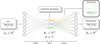 |
Fig. 1 Schematic overview of the autoencoder architecture. Observed spectra xn are given as input and passed through the encoder into a lower dimensional latent space, which is subsequently decoded into the reconstruction |

3.2 Neural network autoencoder
Autoencoders are built to reconstruct the input in the output through a low dimensional representation in the middle of the network. The network consists of an encoder function hn = f (xn), which maps the input data xn ∈ ℝp to a hidden layer describing a latent representation hn ∈ ℝR of the input data. This representation is then passed through the decoder function  , which seeks to reconstruct the input data xn with the reconstruction
  . Autoencoders are typically restricted in various ways to ensure they do not learn the identity function ɡ(f (xn)) = xn. By utilizing appropriate constraints it is possible to force the latent representation hn to take on useful properties. One such constraint is to keep hn at a lower dimension than xn. This will make the autoencoder undercomplete and cause dimensionality reduction, which forces the latent representation to capture only the most salient features of the training data (Goodfellow et al. 2016).
We designed the dimension of the latent representation in the telluric autoencoder to match the number of expected end-members in the trained spectral region such that hn ∈ ℝR. For the HARPS-N data we considered regions with either R = 2 (solar and H2O endmembers) or R = 3 (solar, H2O and O2 end-members) where R ≪ P. After the network training is complete and the network has learned to reconstruct the input signals, the latent representation hn ∈ ℝR can be extracted and interpreted as the endmember abundances wn. While the encoder is responsible for learning the abundances of the underlying components, the decoder is responsible for learning the spectral shape of these components. To enable this interpretation, the decoder must be restricted to perform a single affine transformation:
 (6)
(6)
where W ∈ ℝP×R are the weights of the decoder. Thus, we constructed the decoder without bias terms. With this restriction the decoder weights W can be extracted and interpreted as the endmember spectra M.
3.2.1 Network training
Autoencoders are trained by minimizing a loss function ℒ representing a distance between the input and reconstruction. We used the squared L2 norm resulting in the mean squared error (MSE) of the input and reconstructed spectra as loss function:
 (7)
(7)
Training was performed with gradient descent by updating the network weights to minimize the loss function. Training was carried out for a number of epochs with early stopping, which has been shown to reduce the risk of overfiting (Caruana et al. 2001). The network was trained on non-stitched spectra for the 69 orders separately to retain the high fidelity of the observed spectra and to avoid the complications involved in stitching spectra. The loss of signal at the edges of each order is compensated for by information from the high number of observations used to train the network. Training on all orders took approximately 2 h on an Intel 6 core i7, UHD 630 CPU laptop.
3.2.2 Layer architecture
What follows is a detailed description of the network layers. An overview of the layer architecture of the entire network can be seen in Table 1.
Layer 1 is the input of the network with dimensionality xn ∈ ℝP such that it matches the number of pixels P in the observed spectra used for training. Layer 2 applies dropout during training by randomly zeroing entries, with a chosen probability p, according to a Bernoulli distribution. Random dropout has been shown as an effective regularization technique to reduce over-fitting by preventing complex coadaptations of feature detectors (Hinton et al. 2012).
Layer 3 computes a lower dimensional representation by applying the following transformation:
 (8)
(8)
where a(3) is the activation of layer 3, a(2) is the input given from the previous layer, W(3) are the weights of the layer, b(3) is the bias of the layer, and j is the activation function. The encoder uses a leaky rectified linear unit (LReLU; Xu et al. 2015) as a nonlinear activation function. The encoder can in principle consist of multiple layers with nonlinear activation functions. Similar to Palsson et al. (2018), we found that the structural constraints of the decoder, which are expanded upon in the description of layer 9, limits the advantages of a deep encoder with numerous nonlinear activation functions. We tried various encoder depths and found that differences in learned representations were negligible, while training time was increased significantly with a deep encoder structure. For this reason, the final architecture of our presented network consists of a shallow encoder with a single nonlinear activation function in layer 3.
Layer 4 applies batch normalisation, which is known to accelerate learning by reducing internal covariate shift (LeCun et al. 2012; Ioffe & Szegedy 2015). The batch normalisation operation can be expressed as:
![Mathematical equation: ${\bf{a}}_i^{\left( 4 \right)} = {{{\bf{a}}_i^{\left( 3 \right)} - {\rm{E}}\left[ {{{\bf{\alpha }}^{\left( 3 \right)}}} \right]} \over {\sqrt {Var\left[ {{{\bf{a}}^{\left( 3 \right)}}} \right] + } }}\gamma + \beta ,$](/articles/aa/full_html/2023/09/aa46652-23/aa46652-23-eq12.png) (9)
(9)
where  is the activation of unit i in layer 4 for
  is the activation of unit i from the previous layer, γ and β are learnable parameters, and e is a small number. The expectation and variance can be expressed as:
![Mathematical equation: ${\rm{E}}\left[ {{{\bf{a}}^{\left( 3 \right)}}} \right] = {1 \over R}\sum\limits_{i = 1}^R {{\bf{a}}_i^{\left( 3 \right)}} ,$](/articles/aa/full_html/2023/09/aa46652-23/aa46652-23-eq15.png) (10)
(10)
![Mathematical equation: $Var\left[ {{{\bf{a}}^{\left( 3 \right)}}} \right] = {1 \over R}\sum\limits_{i = 1}^R {{{\left( {{\bf{a}}_i^{\left( 3 \right)} - {\rm{E}}\left[ {{{\bf{a}}^{\left( 3 \right)}}} \right]} \right)}^2}} ,$](/articles/aa/full_html/2023/09/aa46652-23/aa46652-23-eq16.png) (11)
(11)
Layer 5 enforces a nonnegative abundance constraint (ANC):
 (12)
(12)
and normalizes the batch normalized latent abundance tensor a(4) to interval [0, 1] through the following transformation:
 (13)
(13)
where  is the activation of unit i in layer 5.
Layer 6 enforces a lower abundance bound constraint for each endmember to ensure the correct physical representation is learned. Since it can be assumed that the intrinsic solar spectrum remains constant in line depth over the observations (no abundance variation), the solar endmember abundance ω1 is kept fixed:
 (14)
(14)
The H2O and O2 telluric components described by abundance weights ω2 and ω3 change over each observation but are never absent in the observed spectra. This is problematic, since the main feature allowing disentanglement of the solar component from the telluric components is the telluric variability. The constant contribution of each telluric component to the observed spectra complicates this. To ensure the correct representation is learned, the telluric components are normalized to different intervals such that:
![Mathematical equation: ${w_2} \in \,\left[ {{c_2},1} \right],$](/articles/aa/full_html/2023/09/aa46652-23/aa46652-23-eq21.png) (15)
(15)
where c2 is a lower bound on the abundance of the H2O component and:
![Mathematical equation: ${w_3} \in \,\left[ {{c_3},1} \right],$](/articles/aa/full_html/2023/09/aa46652-23/aa46652-23-eq22.png) (16)
(16)
where c3 is a lower bound on the abundance of the O2 component. The lower bounds c2 and c3 on the telluric endmember abundances are defined to represent their respective line depth variability in the spectrum. The H2O component exhibits much larger variability in the observed spectrum than the O2 component, and as such c2 < c3. The value for c2 was determined by inspecting the relative difference between a known H2O line at its strongest and weakest instance in the training set. This was similarly done for a known O2 line. The values used for the HARPS-N training set are c2 = 0.03 and c3 = 0.69.
To incorporate these lower bounds, the abundance tensors are linearly transformed to interval [cr, 1] in layer 6 of the network using the following transformation:
 (17)
(17)
where  is the activation of unit i in layer 6, which are the abundance weights linearly transformed to interval [cr, 1] with cr being the lower bound on the abundance for endmember r. This is the final layer in the latent representation and thus a(6) represents h, which can be extracted as the endmember abundance vector:
![Mathematical equation: ${{\bf{h}}_n} = {{\bf{w}}_n} = {\left[ {{w_{1,n}},{w_{2,n}},{w_{3,n}}} \right]^T}.$](/articles/aa/full_html/2023/09/aa46652-23/aa46652-23-eq24.png) (18)
(18)
Layer 7 performs clamping of endmember spectra (decoder weights), which ensures the extracted endmembers remain normalized and interpretable in relation to the continuum normalized input and output spectra. This is achieved by clamping the weights of the decoder at each forward pass to satisfy:
![Mathematical equation: ${{\bf{m}}_1} \in \left[ {0,1} \right],$](/articles/aa/full_html/2023/09/aa46652-23/aa46652-23-eq25.png) (19)
(19)
![Mathematical equation: ${{\bf{m}}_2} \in \left[ { - 1,0} \right],$](/articles/aa/full_html/2023/09/aa46652-23/aa46652-23-eq26.png) (20)
(20)
![Mathematical equation: ${{\bf{m}}_3} \in \left[ { - 1,0} \right],$](/articles/aa/full_html/2023/09/aa46652-23/aa46652-23-eq27.png) (21)
(21)
where m1 is the solar endmember spectrum, m2 is the H2O end-member spectrum, and m3 is the O2 endmember spectrum. The constraint in Eq. (19) ensures that the extracted solar endmember remains continuum normalized. The constraints in Eqs. (20) and (21) allow the extracted telluric endmembers to be interpreted as transmission spectra, which absorb light from the fixed solar endmember at varying weights controlled by the abundance vector wn from the latent space. The decoder weight constraints act as regularizers guarding against exploding gradients for large learning rates, as the decoder weights can never change significantly between each backward pass.
Layer 8 performs a Doppler shift of the solar component through a shift function. An underlying assumption in the proposed approach is that both the solar spectrum and telluric transmission spectrum remain stationary in the wavelength domain, such that they can be described by the learned weights of the decoder. The observed spectra are wavelength calibrated in the observer rest frame and hence the telluric lines remain stationary. This is however not the case for the solar component due to a slight Doppler shift of the solar spectrum arising from Earth’s rotation and motion around the Sun. The relation between the spectral shift and the velocity is given by:
 (22)
(22)
where v is the velocity, c is the speed of light, λshift is the shifted wavelength, and λrest is the rest wavelength.
The network architecture does not allow the Solar endmember to change over the various observations and thus the Doppler shift of this component in the observed spectra will be caught in the telluric endmembers and cause noise in the extracted spectra. Since the aim is to extract detailed endmembers, this Doppler shift causes an unacceptable amount of noise, especially in regions with strong solar lines. To account for this, the network performs a Doppler shift of the solar endmember toward the solar component reference frame for each observed spectrum. This allows a single solar endmember spectrum to represent the shifted solar component in each observed spectrum. The shifted solar endmember is created by learning a stationary solar end-member in the decoder weights and Doppler shifting it using the barycentric Earth radial velocity (BERV) to match the solar wavelength reference frame in each observed spectrum. This solution reflects the physical nature of the problem, decreases model noise and allows for a better learned representation. To incorporate this solution, a Doppler shifted wavelength axis is computed for each observation according to:
 (23)
(23)
where λrest is the stationary wavelength axis of the solar end-member from the decoder weights and λshift is the new wavelength axis matching the solar component in each observed spectrum. The solar endmember from the decoder weights is then linearly interpolated to this shifted wavelength axis before being combined with the remaining endmembers in the last layer of the network.
Layer 9 is the final layer and computes the output of the network. It has dimensionality  . To ensure that the autoencoder learns a representation that conforms with our LMM in Eq. (5), the decoder function must be restricted to perform a linear transformation from latent representation to reconstruction ɡ(hn) : ℝR → ℝP. Furthermore, to directly extract endmember spectra from the decoder weights, the decoder layer neurons are constructed without bias terms. The decoder thus consists of a single affine transformation:
 (24)
(24)
where a(6) is the activation of layer 6 (the latent abundance representation hn) and W(9) are the weights of the decoder. These weights have dimensionality W(9) ∈ ℝP×R and can be extracted as the endmember spectra M.
Summary of autoencoder layers.
3.2.3 Network initialization
Initialization of weights in neural networks is known to affect both the convergence time and learned representation (Sutskever et al. 2013). We initialized the encoder weights according to the Xavier scheme (Glorot & Bengio 2010). The weights of the decoder can either be initialized in a similar fashion, or can be initialized with weights on a scale similar to the weights the network is expected to learn (Goodfellow et al. 2016). We achieved the latter by initializing the telluric decoder weights with synthetic transmission spectra from molecfit. Additionally, the solar decoder weights were initialized from the observed spectrum in the training set that most closely resembles the intrinsic solar spectrum absent from telluric absorption. This specific observed spectrum was identified as the training observation with the largest mean continuum normalized flux. This is because telluric absorption removes light, and thus the observed continuum normalized spectrum with the least telluric contribution has the largest mean flux. Here it is important to emphasize that we operate on continuum normalized spectra, where non-telluric effects causing differences in the mean raw flux are mostly removed. These non-telluric effects include changes in cloud coverage and instrumental response from observation to observation. Our initialization approach biases the solar decoder weights due to the Doppler shift of the initialization observation. We accounted for this bias when computing the Doppler shifted wavelength axis for each observation by using the relative BERV between the nth observation and the initialization observation. This ensures that the solar decoder weights match the solar wavelength reference frame in each observed spectrum. Both Xavier and custom weight initialization schemes were tested and found to lead to similar learned weights by the end of training. The described custom decoder initialization scheme was however found to speed up model convergence over using Xavier initialization.
3.2.4 Latent space correlation
Spectral regions with strong telluric signal undergo large variation across the training data. This allows the encoder to confidently learn to disentangle the abundance variation of the underlying components. If stitched 1D spectra from the spec-trograph pipeline are used during training, the encoder is able to exploit regions of strong telluric signal to effectively disentangle the individual abundance variation of each endmember. However, we chose to train on non-stitched spectra for the 69 orders separately to retain the high fidelity of the observed spectra. For a number of these orders the telluric signal is weak, which reduces the amount of abundance variation available to learn from the observed spectra. This can cause latent space abundances to become correlated across various endmembers, potentially resulting in entanglement of the endmember spectra. Fortunately, completely disentangling telluric endmembers is not critical for performing accurate telluric correction, as only the combined telluric spectrum is of interest. However, to obtain interpretable disentangled endmembers, we explored means of circumventing the problem. Firstly, the latent space correlation can be avoided by introducing an orthogonality constraint on the abundance vectors during training. However, this is not advisable, as the different telluric components can be naturally correlated through for instance the airmass. Alternatively, it is possible to exploit strong known telluric bands from key orders, such as the O2 γ-band in order 60 (spectral range approximately 6270–6340 Å in air) or the several orders containing significant H2O absorption, such as order 54 of the HARPS-N data (spectral range approximately 5900–5970 Å). These orders contain strong telluric variation and can be stitched on an order with weak tellurics during training to guide the encoder in finding the correct abundances. The guiding is exclusively used to encourage the encoder in learning disentangled abundance vectors, and hence the endmembers are only saved for the spectral region of interest during training (i.e. the decoder weights of the stitched on strong telluric order is not saved after training). Exploiting strong telluric variation from separate orders from the current training order is possible since the different orders have been observed simultaneously and thus represent the same atmospheric conditions. We employed this strategy when training on orders with weak telluric signal to effectively learn the individual abundance variations of O2 and H2O. The endmember correlation topic is further described in Sect. 5.3.
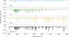 |
Fig. 2 Illustration of the extracted endmembers and an observed solar spectrum for order 60. The extracted endmembers represent from top to bottom the H2O (blue, top), O2 (green) and solar (orange) components of the observed spectrum (black, bottom). |
3.2.5 Hyperparameters
The hyperparameters of the network including learning rate, dropout, momentum, weight decay, and batch normalisation parameters were tuned based on 50 iterations of a Tree-structured Parzen Estimator (TPE) optimization approach carried out with optuna (Akiba et al. 2019) for the individual orders using the MSE reconstruction loss as objective function for minimization. Hyperparameters such as layer dimensions are constrained and were thus not been included in the hyperparameter tuning procedure.
4 Results
The autoencoder has been trained on all 69 orders of the HARPS-N solar observations. We show results from orders containing spectral regions of high interest to the study of exo-planetary atmospheres. These orders exhibit a combination of micro-tellurics in addition to several deep telluric lines originating from H2O and O2 absorption and provide an important challenge for telluric correction frameworks. All results are shown for wavelength measured in air. We report results firstly by showing the extracted endmembers and secondly by demonstrating how the extracted components can be applied to new observations to provide accurate and efficient telluric removal.
4.1 Extracted endmembers
Endmembers M were extracted for each order by fully training the autoencoder on the spectral region of the order and subsequently saving the tensor W ∈ ℝP×R representing the final decoder weights. The associated abundance vector ωn for the nth observation was extracted by saving the latent space tensor hn.
Figure 2 shows the endmembers extracted from order 60. This spectral range contains a combination of strong telluric lines from the O2 γ-band in addition to weaker H2O tellurics. The autoencoder has disentangled the signals from the observed spectrum into its underlying components consisting of the intrinsic solar spectrum and the telluric absorption from H2O and O2. These molecules exhibit different modes of variation in the observed spectra. The network has been allowed to learn their individual abundance variation by using a three-dimensional latent space (extracting three endmembers). The solar endmember is constrained at constant abundance and is not scaled between observations. The telluric components from H2O and O2 are scaled individually by their learned abundance vectors for each observation to match the atmospheric conditions at the time of the observation. For visibility, Fig. 2 includes an observed spectrum with strong telluric contamination and the H2O and O2 endmembers have been scaled with their respective learned abundances from the latent space for the illustrated observation. Note how the network has learned to disentangle the observed spectrum into interpretable components even in highly mixed spectral regions such as 6750–6850 Å, where significant solar lines are interlaced with deep O2 tellurics and weaker H2O lines. This is achieved by exploiting how these spectral components vary individually according to the physical laws that govern them.
We further investigate the interpretability of the extracted components by inspecting learned endmember abundance correlation with airmass. While O2 abundance is expected to correlate strongly with airmass, H2O abundance correlates more strongly with atmospheric water vapor content. Figure 3 shows scatter plots of the learned abundances with the corresponding airmass for each observation. As expected from the physical model of the system, the learned abundance of the O2 component shows a strong linear correlation with airmass, while the H2O component shows a much weaker correlation.
Additional extracted endmembers for order 53 and 54 can be found in Figs. A.1 and A.2. Firstly, order 53 contains the prominent Na doublet in addition to a wealth of micro-tellurics from H2O. The network has disentangled the observed spectra into a fixed solar endmember and a telluric H2O endmember. Order 53 contains a number of lines where H2O tellurics are positioned on top of strong solar lines. This is for instance the case between 5880 Åand 5900 Å, where strong H2O tellurics occur in the same spectral region as the prominent solar Na lines. We initially expected such mixed lines to compromise the quality of the extracted endmembers, but as we demonstrate in Sect. 4.2, the extracted solar and telluric components have been effectively disentangled allowing for accurate telluric correction even in spectral regions of mixed stellar and telluric signal. Figure A.2 shows endmembers for order 54, which contains numerous water tellurics as well as strong solar lines.
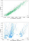 |
Fig. 3 Scatter plots of airmass and the telluric abundances learned by the autoencoder for order 60 of the HARPS-N solar observations. The O2 endmember abundances (top, green) show a clear linear relationship with airmass, while the H2O endmember abundances (bottom, blue) show a much weaker correlation with airmass. |
4.2 Telluric correction
Telluric correction removes tellurics by dividing the observed spectrum with a combined telluric transmission spectrum. In this section we demonstrate how the extracted endmembers can be applied to new observations to carry out accurate and efficient telluric correction. We do this by performing telluric correction on a collection of observations from the HARPS-N spectrograph originating both from solar observations as well as stellar observations of relevance to the detection of exoplanetary atmospheric features.
4.2.1 Telluric correction on validation observation
We start by demonstrating telluric correction on a validation solar observation with strong telluric contamination from HARPS-N. The validation observation is from November 2020 and TAU has not seen the observation during training. As a baseline for comparison we perform telluric correction of the same observation using the state-of-the-art synthetic telluric correction approach molecfit. We computed the molecfit telluric transmission spectrum using version 1.5.9 of molecfit on an HPC cluster (DTU Computing Center3) using a 10 core Intel Xeon E5-2660v3, Huawei XH620 V3 node and utilized atmospheric measurements from the time of the observation in addition to a fit to the stitched version of the observation from the HARPS-N pipeline. We computed the TAU correction on an Intel 6 core i7, UHD 630 CPU laptop using the extracted telluric components, which were converted back from log-space to represent standard transmission spectra. Autoencoder telluric abundance weights were found using a least squares fit to known telluric lines in the spectrum. No external atmospheric measurements were used during the autoencoder correction. We interpolated the telluric transmission spectra of TAU and molecfit to the wavelength axis of the observed spectrum to represent standard telluric correction procedure. The molecfit correction took approximately 30 min to compute (separate from the additional time needed to optimize molecfit parameters to improve the quality of the fit), while the autoencoder correction took less than 0.2 s.
Figure 4 shows the correction around the solar Na doublet in order 53. This region contains numerous deep isolated H2O tellurics as well as telluric lines interwoven with intrinsic solar lines. Both TAU and molecfit have managed to correct for the telluric contamination by removing most of the telluric lines to continuum level. For an isolated telluric line, a perfect correction would be to the continuum level leaving no residual from the correction. In this spectral region molecf it is clearly over-correcting a H2O line at 5886 Å by correcting it above continuum level and leaving a large residual. The problem with this particular line is discussed in the literature (Cabot et al. 2020), and is possibly caused by an extra entry in the line list used by molecfit. TAU does not make use of external factors like molecular line list and has managed to correct this line to continuum level. A similar, but less significant over-correction by molecf it can be seen on the H2Oline at 5909 Å. While we have observed a number of similar small over-corrections by molecf it across the spectrum, they are not indicative of the general correction performance of molecfit on lines where the correct external parameters are used.
Figure 5 shows telluric correction around the solar Hα line in order 64. This particular spectral range is of interest for exo-planetary research and poses a difficult challenge for telluric correction frameworks due to the large number of deep telluric lines. Both molecfit and TAU have corrected the observed spectrum uncovering the intrinsic solar spectrum without indications of over-corrections. However, as is visible for a number of the deepest telluric lines, molecfit slightly under-corrects and leaves residuals from the correction, while TAU generally removes the telluric lines with higher accuracy.
Figure 6 shows a closer look at the fitted telluric transmission spectra and corresponding corrections of the isolated deep 6543.9 Å telluric line also visible in Fig. 5. This telluric line is particularly challenging due to its significant depth. Since an ideal correction would leave no residual, we can measure the residual of the correction and use it as a metric for correction performance. The residuals are measured as the root mean squared errors (RMSE) from continuum level. The autoencoder residual (blue) is significantly smaller than the molecfit residual (red). As can be seen from the overlaid molecfit and autoencoder transmission spectra, the differences in residuals emerge due to discrepancies both in the depth as well as the exact wavelength position of the line center in the transmission spectra used for the correction.
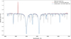 |
Fig. 4 Comparison of corrected spectra around the solar Na doublet (order 53). The corrections are computed using either autoencoder extracted tellurics or molecfit. |
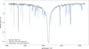 |
Fig. 5 Comparison of corrected spectra in order 64. The corrections are computed using either autoencoder extracted tellurics or molecf it for H2O lines in the spectral region around Hα. |
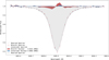 |
Fig. 6 Residuals from telluric correction. The correction is performed on the validation spectrum with TAU and molecfit for a prominent H2O telluric close to the Hα solar line shown in Fig. 5. An ideal correction would result in no residual (flat line at continuum level). |
4.2.2 Temporal generalizability of correction performance
The validation spectrum has been observed at a point close in time to the training data of the autoencoder. It is possible that seasonal atmospheric effects can impact the correction performance of the extracted tellurics. For this reason we performed numerous corrections on a large number of HARPS-N solar observations across various observing seasons to demonstrate the general correction performance of the autoencoder.
We chose 100 random observations from each observing season between 2015 and 2018 resulting in 400 observations of the solar spectrum. We then performed telluric correction on each of them using the autoencoder tellurics. All 400 corrections (across the entire observed spectrum) were computed in a total time of less than 1 min on an Intel 6 core i7, UHD 630 CPU laptop. We have not computed molecfit corrections on these observations due to the significant computational expense involved in performing molecfit corrections on several hundred observations (and the additional time for optimizing parameters). Table 2 shows the mean RMSE of the residuals for various telluric lines across each year of observations. The table also shows the residual on the single 2020 validation observation for reference. TAU has smaller residual than molecfit on the validation observation for all three spectral regions. The mean autoencoder residual for each annual observing season is also less than the molecfit correction in each spectral region. TAU generally has a smaller residual on the 2020 validation observation than the mean residual across the previous observing seasons, this is however not the case for telluric lines in order 54 (spectral range 5945.1–5946.3 Å). Overall, the correction performance shows no clear temporal trend.
Correction performance in three spectral regions with strong tellurics.
4.2.3 Endmember correlation
Figure 7 shows telluric correction in a region of combined H2O and O2 tellurics in order 60. The top panel shows the residuals from the correction on the validation observation, while the bottom panel shows the individual spectra for H2O and O2 used by TAU. In the left side of the figure a small H2O telluric is positioned on top of the wing of a stronger O2 telluric. TAU has modeled the combined observed telluric transmission spectrum in this region by combining the lines. Weak H2O tellurics are visible under each of the two stronger O2 tellurics. The location of these weak tellurics could indicate that the autoencoder has not fully disentangled the H2O and O2 telluric spectra from each other. This is further discussed in Sect. 5.3.
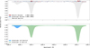 |
Fig. 7 Correction of H2O and O2 tellurics. Top: observed validation spectrum and residuals from telluric correction with TAU and molecfit in a region with H2O and O2 tellurics in order 60. Bottom: autoencoder endmembers for H2O and O2 in the same spectral region. |
4.2.4 Impact of training data
TAU was trained on solar observations, which are comparatively cheap to obtain. We also envision the possibility of training the autoencoder on nonsolar data in situations where a spectrograph is not fed by a solar telescope. Such data are bound to have larger BERVs, which could aid in disentangling the stellar and telluric components from each other. On the other hand, nonsolar data also have lower S/N, which would require a larger number of training observations to obtain high endmember fidelity. Obtaining nonsolar data is expensive, and it is important to know how the amount of training data impacts the generated results. For this reason, we retrained TAU on various amounts of training data and performed corrections with the resulting extracted tellurics.
Table 3 shows the impact on correction performance when reducing the size of the training data. We did this by randomly subsampling the original 838 observations to generate training sets of respectively 400 and 200 observations. We performed the sampling 5 times for both cases and report the mean RMSE and standard deviations for corrections on the 400 observations from 2015 to 2018. This results in 2000 corrections made from the tellurics extracted from networks trained on either 400 or 200 observations. The correction performance can be observed to decrease slightly with the size of the training data. This is expected, as feeding the autoencoder additional training data allows it to learn a more detailed telluric spectrum, leading to more accurate corrections. The correction performance is however quite stable across the training set sizes, indicating that the salient features of the data can be learned from a modest training set. Thus, the size of the training set is not directly critical in obtaining an accurate telluric spectrum. Rather, the critical part is to obtain sufficient abundance variation within the training data to learn the telluric spectrum across various atmospheric conditions. Generally, more training data carries more variation, but this is not necessarily the case. For instance numerous training observations recorded during the same night may not contain sufficient atmospheric variation to constitute a good training set.
Correction performance dependence on training data size.
4.2.5 Systematic correction performance
Natural noise artifacts like cosmic rays and photon noise impacts the residual. We demonstrate the systematic correction performance of TAU in Fig. 8, where telluric correction on a series of tellurics in order 54 is compared between a single residual from the 2020 validation observation and the combined residual from numerous corrections. The top panel shows the correction performance on the validation observation, where small correction artifacts are visible for molecfit and autoencoder corrections. The bottom panel shows the combined residual from averaging residuals at each wavepoint over corrections performed by TAU on the 400 observations from 2015 to 2018 in the same spectral region.
Small systematic correction artifacts by TAU can be seen close to the 5946 Å line, where several telluric lines are superimposed on top of each other. In this region, the autoencoder has a slight systematic over-correction effect. Overall the correction residual is within 1 per cent of the continuum level on all telluric lines shown in the figure. We found similar systematic correction performance within 1 per cent of the continuum level in telluric lines across the observed spectrum in the analyzed orders (53, 54, 60 and 64).
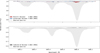 |
Fig. 8 Correction of H2O tellurics. Top: residuals from telluric correction with TAU and molecfit on the validation observation for tellurics in order 54. Bottom: combined residual in the same spectral region from correction of 400 observations between 2015 and 2018 performed with TAU. Combination is performed by averaging the residuals for each wave-point. The single observed spectrum from the top plot is shown for visual comparison. |
4.2.6 Telluric correction for exoplanetary atmosphere retrieval
TAU was trained on solar observations but is intended to be used for correction of night time observations. To demonstrate the ability to perform corrections on night time data with much lower S/N, we replicated the detection of Na in the atmosphere of HAT-P-70b (Zhou et al. 2019) by Bello-Arufe et al. (2022), where the authors analyzed 40 spectra collected during a transit event of this ultra-hot Jupiter on 18 Dec 2020 between 21:28 and 02:10 UTC. The Na doublet is in a spectral region particularly sensitive to telluric absorption, so this is a good exercise to test the applicability of TAU to exoplanet atmospheric retrieval. The 40 spectra were first corrected for tellurics using either molecfit or TAU. We then followed the same transmission spec-troscopy analysis described in Bello-Arufe et al. (2022). The result is shown in Fig. 9. The molecfit corrections were performed in the same manner as for the solar observations, with a total computational time of approximately 7 h (excluding additional time for optimizing parameters manually). We inspected the molecfit input line list and removed the potential source of the overcorrection near 5886 Å, as already done in Bello-Arufe et al. (2022). TAU corrections were performed using the extracted tellurics without manual parameter optimization with a total computational time for the 40 corrections of approximately 10 s.
The retrieved Na D1 and Na D2 lines from the observations corrected with either molecfit or TAU are shown in Tables 4 and 5. Due to the limited S/N of this data, we observe no significant differences in the results obtained with either TAU or molecfit corrections.
Na D1 line results for the ultra-hot Jupiter HAT-P-70b using molecfit or TAU for telluric correction.
Na D2 line results for the ultra-hot Jupiter HAT-P-70b using molecfit or TAU for telluric correction.
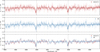 |
Fig. 9 Transmission spectroscopy for the Na I doublet. The spectroscopy is performed using molecfit corrected spectra (top panel, red) and Autoencoder corrected spectra (middle panel, blue). The unbinned transmission spectra from either approach is shown in respectively light red and light blue while the binned master transmission spectra are shown as solid red and solid blue error bars. Each master transmission spectrum is fitted with a Gaussian model (solid red and solid blue lines). The vertical dotted gray lines show the theoretical location of each spectral line. The bottom panel shows a direct comparison of the binned master transmission spectra and the Gaussian models from either molecfit and TAU. |
5 Discussion
In this section, we discuss the results and touch on the advantages and limitations of the autoencoder model in addition to laying out the future work for our approach.
5.1 Comparison with molecfit
Our comparisons reveal how the autoencoder extracted spectra closely resemble the synthetic transmission spectra of H2O and O2 from molecfit. All telluric lines modelled by molecfit are also present in the autoencoder telluric endmembers. The two approaches however exhibit small differences regarding the depth, width and spectral location of lines.
The autoencoder telluric endmembers better match the actual width, depth and spectral position of observed tellurics leading to more accurate correction. Furthermore, corrections with TAU are performed approximately 10 000 times faster than molecfit. This difference in compute time is significant and makes TAU much more feasible for correction of multiple spectra. Finally, the autoencoder approach can be used as a complementary data-driven validation tool to inspect the accuracy of synthetic approaches like molecfit, for instance by bringing attention to over-correction artifacts caused by line lists entry errors, not only in obvious cases like the 5886 Å telluric line in Fig. 4, but also in more subtle cases like the 5909 Å line in the same figure.
5.2 Advantages
The autoencoder approach for extracting telluric transmission spectra has certain advantages over other methods with the same aim. Firstly, since the approach is data-driven, it is possible to extract the combined telluric spectrum without relying on the precision of atmospheric measurements at the time of the observation, as well as external factors like molecular line lists. This is a major advantage over synthetic models, which are inherently limited by the precision of such factors. Furthermore, due to the high S/N and resolution of the training data from HARPS-N, it is possible to extract the spectral shape and location of telluric lines with very high accuracy. This type of accuracy on correction of telluric lines is increasingly important as we get closer to the 10 cm/s RV barrier for detecting Earth-like exoplanets.
Compared to other data-driven methods the autoencoder approach has the advantage that it can work and learn from immense datasets by training with mini-batch gradient descent. Traditionally neural networks have poor interpretability, but the highly constrained nature of the network architecture causes the learned representation to assume very specific properties, naturally leading to better interpretability of both the latent representation, as well as the extracted endmember spectra. The network constraints are highly customizable, allowing the framework to be adapted to other wavelength intervals or settings of spectral unmixing.
5.3 Limitations
For orders where the telluric components only exhibit minor variation, the encoder has difficulty learning the abundance variation. This is evident for order 60, where the H2O component is much weaker than the O2 component and thus constitutes less of the overall flux variation in the region. This caused the encoder to entangle the telluric abundances of H2O and O2, which lead to the decoder disentangling their spectra.
This correlation of features occurring in the encoding stage of an autoencoder trained with MSE is a known issue, which in the literature has been tackled by introducing either an orthogonality regularization term to the loss function (Wang et al. 2019) or by modeling the underlying low dimensional manifold as a product of submanifolds, each modeling a different factor of variation (Fumero et al. 2021). With the physical assumption that the H2O and O2 telluric components share at least a minor correlation through airmass, we circumvented the issue by stitching on a spectral region with strong tellurics, causing a disentanglement of the H2O and O2 endmembers while still allowing them to be correlated. The latent space correlation between the learned endmember abundances and consequently spectra, is likely not critical, as the correction of telluric lines in observed spectra is performed with the combined spectrum from all telluric components. From Fig. 7, we see how the combination of telluric components from H2O and O2 corrects for telluric lines in an unseen observed spectrum. As is evident, the correction is performed with high accuracy, suggesting the autoencoder can still accurately represent observed tellurics through a combination of moderately entangled telluric components. The question of whether the solar component has been fully disentangled (or to which degree) from the telluric components however remains.
Another potential limitation lies in the assumption that the components of the telluric spectrum can be seen as a fixed spectra scaled with an abundance weight. This assumption is based on the fact that temperature and pressure variations in the Earth atmosphere are likely small enough that the telluric spectrum can be represented like this. If the relative shape or spectral location of lines in the transmission spectrum of a molecular species undergo large temporal changes, then this assumption is unjustified. This could potentially be caused by large scale pressure and temperature variations in the Earth atmosphere. To retain high correction performance, this would mean that extracted endmembers used for correction would have to be learned from solar spectra observed relatively closely in time to the observation on which telluric correction is performed. However, our experiments on corrections across annual observing seasons show that no significant performance deterioration is apparent from temporal evolution. Finally, our physical model assumes an ideal spectrograph. If the instrumental profile changes significantly over time then our physical model is not valid. This makes TAU most applicable for well-stabilized spectrographs.
5.4 Future work
Future work includes extending TAU to other spectrographs and spectral ranges. This includes testing the approach on regions of saturated telluric lines in the redder part of the spectrum, which is currently a significant challenge for ground-based astrophysics. Furthermore, the telluric weights used during telluric correction on new observations with the extracted endmembers are currently found using a least squares fit to known telluric lines in the spectrum. This could be improved by building TAU into a full forward model which includes stellar and telluric spectrum, such that these weights can be learned from all telluric lines simultaneously. This approach would be feasible due to the fast computation time of TAU.
6 Conclusion
We have introduced TAU, an open-source library that demonstrates a novel approach for extracting a compressed representation of observed solar spectra from HARPS-N using a highly constrained neural network autoencoder. We have shown how this representation can be used to extract endmembers that directly relate to the intrinsic solar spectrum as well as telluric transmission spectra of H2O and O2. After the autoencoder representation has been computed for a given spectrograph, the extracted components can be used to perform quick and accurate telluric correction on any observations from the same spectro-graph. By comparing with molecfit, we have shown that the autoencoder extracted tellurics can be used as a master telluric spectrum with correction performance rivaling molecfit in large regions of the spectrum at a significantly reduced computational expense. TAU is data-driven and is thereby not affected by external factors like line list precision. This leads to improved correction accuracy over molecfit in various regions of the spectrum. TAU can be trained on observed solar spectra from any spectrograph and in this way extract a high-precision telluric profile for the given spectrograph. The extracted profile can be used to mitigate the telluric component in new observations, which could aid in the detection of faint radial velocity signals and atmospheric features of Earth analog exoplanets observed from ground-based telescopes.
Acknowledgements
We would like to thank HARPS-N for providing the public solar data used to train TAU. These data are based on observations made with the Italian Telescopio Nazionale Galileo (TNG) operated on the island of La Palma by the Fundación Galileo Galilei of the INAF (Istituto Nazionale di Astrofisica) at the Spanish Observatorio del Roque de los Muchachos of the Instituto de Astrofisica de Canarias. Without this vast quantity of high S/N data our approach would not be feasible. Furthermore, we would like to thank molecfit for providing their open-source synthetic telluric correction framework, which we have not only used for initializing the autoencoder weights, but also for validating our extracted tellurics. Without a detailed synthetic telluric spectrum computed based on physical models, it would be significantly more complicated to validate our data-driven approach. Furthermore, we would like to acknowledge the DTU HPC cluster, which we have used for computing molecfit corrections. A portion of this research was carried out at the Jet Propulsion Laboratory, California Institute of Technology, under a contract with the National Aeronautics and Space Administration (80NM0018D0004).
Appendix A Additional extracted endmembers
We provide additional results for extracted endmembers for order 53 and 54 in Figs. A.1 and A.2.
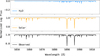 |
Fig. A.1 Extracted endmembers and an observed solar spectrum for order 53. The network has been trained using a two-dimensional latent space resulting in R = 2 endmembers. The extracted endmembers represent the H2O (top, blue) and solar (middle, orange) components of the observed spectrum (bottom, black). |
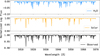 |
Fig. A.2 Extracted endmembers and an observed solar spectrum for order 54. The network has been trained using a two-dimensional latent space resulting in R = 2 endmembers. The extracted endmembers represent the H2O (top, blue) and solar (middle, orange) components of the observed spectrum (bottom, black). |
References
- Akiba, T., Sano, S., Yanase, T., Ohta, T., & Koyama, M. 2019, in Proceedings of the 25th ACM SIGKDD International Conference on Knowledge Discovery & Data Mining, 2623 [CrossRef] [Google Scholar]
- Artigau, É., Astudillo-Defru, N., Delfosse, X., et al. 2014, in Observatory Operations: Strategies, Processes, and Systems V, 9149, 914905 [CrossRef] [Google Scholar]
- Bean, J. L., Seifahrt, A., Hartman, H., et al. 2010, ApJ, 713, 410 [NASA ADS] [CrossRef] [Google Scholar]
- Bedell, M., Hogg, D. W., Foreman-Mackey, D., Montet, B. T., & Luger, R. 2019, AJ, 158, 164 [Google Scholar]
- Bello-Arufe, A., Cabot, S. H., Mendonça, J. M., Buchhave, L. A., & Rathcke, A. D. 2022, AJ, 163, 96 [NASA ADS] [CrossRef] [Google Scholar]
- Bender, C. F., Mahadevan, S., Deshpande, R., et al. 2012, ApJ, 751, L31 [NASA ADS] [CrossRef] [Google Scholar]
- Bertaux, J.-L., Lallement, R., Ferron, S., Boonne, C., & Bodichon, R. 2014, A&A, 564, A46 [NASA ADS] [CrossRef] [EDP Sciences] [Google Scholar]
- Bourlard, H., & Kamp, Y. 1988, Biol. Cybernet., 59, 291 [CrossRef] [Google Scholar]
- Cabot, S. H. C., Madhusudhan, N., Welbanks, L., Piette, A., & Gandhi, S. 2020, MNRAS, 494, 363 [Google Scholar]
- Caruana, R., Lawrence, S., & Giles, L. 2001, Adv. Neural Inform. Process. Syst., 402 [Google Scholar]
- Clough, S., Shephard, M., Mlawer, E., et al. 2005, J. Quant. Spectrosco. Radiat. Transfer, 91, 233 [NASA ADS] [CrossRef] [Google Scholar]
- Cosentino, R., Lovis, C., Pepe, F., et al. 2012, SPIE Conf. Ser., 8446, 84461V [Google Scholar]
- Cunha, D., Santos, N. C., Figueira, P., et al. 2014, A&A, 568, A35 [NASA ADS] [CrossRef] [EDP Sciences] [Google Scholar]
- Dumusque, X., Cretignier, M., Sosnowska, D., et al. 2021, A&AS, 648, A103 [NASA ADS] [CrossRef] [EDP Sciences] [Google Scholar]
- Fischer, D. A., Anglada-Escude, G., Arriagada, P., et al. 2016, PASP, 128, 066001 [Google Scholar]
- Fumero, M., Cosmo, L., Melzi, S., & Rodolà, E. 2021, ArXiv e-prints [arXiv:2103.01638] [Google Scholar]
- Glorot, X., & Bengio, Y. 2010, in Proceedings of the Thirteenth International Conference on Artificial Intelligence and Statistics, JMLR Workshop and Conference Proceedings, 249 [Google Scholar]
- Goodfellow, I., Bengio, Y., Courville, A., & Bengio, Y. 2016, Deep Learning, 1 (Cambridge: MIT Press), 1 [Google Scholar]
- Gullikson, K., Dodson-Robinson, S., & Kraus, A. 2014, AJ, 148, 53 [NASA ADS] [CrossRef] [Google Scholar]
- Heylen, R., Parente, M., & Gader, P. 2014, IEEE J. Sel. Top. Appl. Earth Observ.Rem. Sensing, 7, 1844 [NASA ADS] [CrossRef] [Google Scholar]
- Hinton, G. E., & Salakhutdinov, R. R. 2006, Science, 313, 504 [Google Scholar]
- Hinton, G. E., & Zemel, R. S. 1994, Adv. Neural Inform. Process. Syst., 6, 3 [Google Scholar]
- Hinton, G. E., Srivastava, N., Krizhevsky, A., Sutskever, I., & Salakhutdinov, R. R. 2012, ArXiv e-prints [arXiv:1207.0580] [Google Scholar]
- Ioffe, S., & Szegedy, C. 2015, in International Conference on Machine Learning, PMLR, 448 [Google Scholar]
- Kausch, W., Noll, S., Smette, A., et al. 2015, A&A, 576, A78 [NASA ADS] [CrossRef] [EDP Sciences] [Google Scholar]
- Langeveld, A. B., Madhusudhan, N., Cabot, S. H., & Hodgkin, S. T. 2021, MNRAS, 502, 4392 [NASA ADS] [CrossRef] [Google Scholar]
- LeCun, Y. A., Bottou, L., Orr, G. B., & Müller, K.-R. 2012, in Neural Networks: Tricks of the Trade (Springer), 9 [CrossRef] [Google Scholar]
- Leet, C., Fischer, D. A., & Valenti, J. A. 2019, AJ, 157, 187 [NASA ADS] [CrossRef] [Google Scholar]
- Palsson, B., Sigurdsson, J., Sveinsson, J. R., & Ulfarsson, M. O. 2018, IEEE Access, 6, 25646 [CrossRef] [Google Scholar]
- Smette, A., Sana, H., Noll, S., et al. 2015, A&A, 576, A77 [NASA ADS] [CrossRef] [EDP Sciences] [Google Scholar]
- Somers, B., Asner, G. P., Tits, L., & Coppin, P. 2011, Rem. Sens. Environ., 115, 1603 [NASA ADS] [CrossRef] [Google Scholar]
- Sutskever, I., Martens, J., Dahl, G., & Hinton, G. 2013, in International Conference on Machine Learning, PMLR, 1139 [Google Scholar]
- Tamuz, O., Mazeh, T., & Zucker, S. 2005, MNRAS, 356, 1466 [Google Scholar]
- Vacca, W. D., Cushing, M. C., & Rayner, J. T. 2003, PASP, 115, 389 [NASA ADS] [CrossRef] [Google Scholar]
- Wang, S. X., Latouf, N., Plavchan, P., et al. 2022, AJ, 164, 211 [NASA ADS] [CrossRef] [Google Scholar]
- Wang, W., Yang, D., Chen, F., et al. 2019, IEEE Access, 7, 62421 [CrossRef] [Google Scholar]
- Xu, B., Wang, N., Chen, T., & Li, M. 2015, ArXiv e-prints [arXiv:1505.00853] [Google Scholar]
- Zhao, H., & Zhao, X. 2019, Eur. J. Rem. Sens., 52, 277 [NASA ADS] [CrossRef] [Google Scholar]
- Zhou, G., Huang, C. X., Bakos, G. Á., et al. 2019, AJ, 158, 141 [Google Scholar]
Our code is publicly available at https://github.com/RuneDK93/telluric-autoencoder
All Tables
Na D1 line results for the ultra-hot Jupiter HAT-P-70b using molecfit or TAU for telluric correction.
Na D2 line results for the ultra-hot Jupiter HAT-P-70b using molecfit or TAU for telluric correction.
All Figures
|
Fig. 1 Schematic overview of the autoencoder architecture. Observed spectra xn are given as input and passed through the encoder into a lower dimensional latent space, which is subsequently decoded into the reconstruction |
| In the text | |
|
Fig. 2 Illustration of the extracted endmembers and an observed solar spectrum for order 60. The extracted endmembers represent from top to bottom the H2O (blue, top), O2 (green) and solar (orange) components of the observed spectrum (black, bottom). |
| In the text | |
|
Fig. 3 Scatter plots of airmass and the telluric abundances learned by the autoencoder for order 60 of the HARPS-N solar observations. The O2 endmember abundances (top, green) show a clear linear relationship with airmass, while the H2O endmember abundances (bottom, blue) show a much weaker correlation with airmass. |
| In the text | |
|
Fig. 4 Comparison of corrected spectra around the solar Na doublet (order 53). The corrections are computed using either autoencoder extracted tellurics or molecfit. |
| In the text | |
|
Fig. 5 Comparison of corrected spectra in order 64. The corrections are computed using either autoencoder extracted tellurics or molecf it for H2O lines in the spectral region around Hα. |
| In the text | |
|
Fig. 6 Residuals from telluric correction. The correction is performed on the validation spectrum with TAU and molecfit for a prominent H2O telluric close to the Hα solar line shown in Fig. 5. An ideal correction would result in no residual (flat line at continuum level). |
| In the text | |
|
Fig. 7 Correction of H2O and O2 tellurics. Top: observed validation spectrum and residuals from telluric correction with TAU and molecfit in a region with H2O and O2 tellurics in order 60. Bottom: autoencoder endmembers for H2O and O2 in the same spectral region. |
| In the text | |
|
Fig. 8 Correction of H2O tellurics. Top: residuals from telluric correction with TAU and molecfit on the validation observation for tellurics in order 54. Bottom: combined residual in the same spectral region from correction of 400 observations between 2015 and 2018 performed with TAU. Combination is performed by averaging the residuals for each wave-point. The single observed spectrum from the top plot is shown for visual comparison. |
| In the text | |
|
Fig. 9 Transmission spectroscopy for the Na I doublet. The spectroscopy is performed using molecfit corrected spectra (top panel, red) and Autoencoder corrected spectra (middle panel, blue). The unbinned transmission spectra from either approach is shown in respectively light red and light blue while the binned master transmission spectra are shown as solid red and solid blue error bars. Each master transmission spectrum is fitted with a Gaussian model (solid red and solid blue lines). The vertical dotted gray lines show the theoretical location of each spectral line. The bottom panel shows a direct comparison of the binned master transmission spectra and the Gaussian models from either molecfit and TAU. |
| In the text | |
|
Fig. A.1 Extracted endmembers and an observed solar spectrum for order 53. The network has been trained using a two-dimensional latent space resulting in R = 2 endmembers. The extracted endmembers represent the H2O (top, blue) and solar (middle, orange) components of the observed spectrum (bottom, black). |
| In the text | |
|
Fig. A.2 Extracted endmembers and an observed solar spectrum for order 54. The network has been trained using a two-dimensional latent space resulting in R = 2 endmembers. The extracted endmembers represent the H2O (top, blue) and solar (middle, orange) components of the observed spectrum (bottom, black). |
| In the text | |
Current usage metrics show cumulative count of Article Views (full-text article views including HTML views, PDF and ePub downloads, according to the available data) and Abstracts Views on Vision4Press platform.
Data correspond to usage on the plateform after 2015. The current usage metrics is available 48-96 hours after online publication and is updated daily on week days.
Initial download of the metrics may take a while.