| Issue |
A&A
Volume 677, September 2023
|
|
|---|---|---|
| Article Number | A114 | |
| Number of page(s) | 34 | |
| Section | Extragalactic astronomy | |
| DOI | https://doi.org/10.1051/0004-6361/202346192 | |
| Published online | 15 September 2023 | |
A MUSE/VLT spatially resolved study of the emission structure of Green Pea galaxies
1
Instituto de Astrofísica de Andalucía, CSIC, Apartado de correos 3004, 18080 Granada, Spain
e-mail: aarroyo@iaa.es
2
Centro Astronómico Hispano en Andalucía, Observatorio de Calar Alto, Sierra de los Filabres, 04550 Gérgal, Spain
3
Instituto de Investigación Multidisciplinar en Ciencia y Tecnología, Universidad de La Serena, Raúl Bitrán, 1305 La Serena, Chile
4
Departamento de Astronomía, Universidad de La Serena, Av. Juan Cisternas, 1200 Norte, La Serena, Chile
5
Department of Astronomy, Stockholm University, AlbaNova University Centre, 106 91 Stockholm, Sweden
Received:
20
February
2023
Accepted:
8
June
2023
Green Pea galaxies (GPs) present among the most intense starbursts known in the nearby Universe. These galaxies are regarded as local analogs of high-redshift galaxies, making them a benchmark in the understanding of the star formation processes and the galactic evolution in the early Universe. In this work, we performed an integral field spectroscopic (IFS) study for a set of 24 GPs to investigate the interplay between its ionized interstellar medium (ISM) and the massive star formation that these galaxies present. Observations were taken in the optical spectral range (λ4750 Å–λ9350 Å) with the MUSE spectrograph attached to the 8.2 m telescope VLT. Spatial extension criteria were employed to verify which GPs are spatially resolved in the MUSE data cubes. We created and analyzed maps of spatially distributed emission lines (at different stages of excitation), continuum emission, and properties of the ionized ISM (e.g., ionization structure indicators, physical-chemical conditions, dust extinction). We also took advantage of our IFS data to produce integrated spectra of selected galactic regions in order to study their physical-chemical conditions. Maps of relevant emission lines and emission line ratios show that higher-excitation gas is preferentially located in the center of the galaxy, where the starburst is present. The continuum maps, with an average angular extent of 4″, exhibit more complex structures than the emission line maps. However, the [O III]λ5007 Å emission line maps tend to extend beyond the continuum images (the average angular extent is 5.5″), indicating the presence of low surface brightness ionized gas in the outer parts of the galaxies. Hα/Hβ, [S II]/Hα, and [O I]/Hα maps trace low-extinction, optically thin regions. The line ratios [O III]/Hβ and [N II]/Hα span extensive ranges, with values varying from 0.5 dex to 0.9 dex and from −1.7 dex to −0.8 dex, respectively. Regarding the integrated spectra, the line ratios were fit to derive physical properties including the electron densities ne = 30 − 530 cm−3, and, in six GPs with a measurable [O III]λ4363 Å line, electron temperatures of Te = 11 500 K–15 500 K, so the direct method was applied in these objects to retrieve metallicities 12 + log(O/H)≃8. We found the presence of the high-ionizing nebular He IIλ4686 Å line in three GPs, where two of them present among the highest sSFR values (> 8 × 10⁸ yr−1) in this sample. Non-Wolf-Rayet (WR) features are detected in these galaxy spectra.
Key words: HII regions / galaxies: starburst / galaxies: ISM / galaxies: star formation / galaxies: evolution / ISM: abundances
Note to the reader: the 2 original parts of Table F.1 were inadvertently merged, and the 2nd occurrence of GP18 was for GP19 in Tables F.1 and F.2. Also, reference Lumbreras-Calle et al. (2022) was missing. Following the publication of the corrigendum, this was corrected on 9 October 2023.
© The Authors 2023
 Open Access article, published by EDP Sciences, under the terms of the Creative Commons Attribution License (https://creativecommons.org/licenses/by/4.0), which permits unrestricted use, distribution, and reproduction in any medium, provided the original work is properly cited.
This article is published in open access under the Subscribe to Open model. Subscribe to A&A to support open access publication.
1. Introduction
The cosmic dawn (6 ≲ z ≲ 10) marks a major phase transition of the Universe, during which the “first light” [metal-free stars (or the so-called PopIII-stars) and the subsequent formation of numerous low-mass, extremely metal-poor galaxies] appeared, putting an end to the dark ages. The details of the reionization history reflects the nature of these first sources, which is just starting to be constrained with the James Webb Space Telescope (JWST; e.g., Curtis-Lake et al. 2023; Robertson et al. 2023; Naidu et al. 2022). However, exactly when and how the Universe was reionized remains one of the most important questions of modern astrophysics, and that will be explored during the next decades.
An immediately accessible approach to better understand the first sources is to identify galaxies at lower redshifts with properties similar to galaxies in the very early Universe (e.g., Schaerer et al. 2022; Chen et al. 2023). Among these local analogs, we find the objects known as GPs, which are a subset of galaxies inside the extreme emission line galaxies’ (EELGs’) set (e.g., Pérez-Montero et al. 2021; Breda et al. 2022; Iglesias-Páramo et al. 2022; Lumbreras-Calle et al. 2022). GPs are compact starbursts commonly found at redshift z ∈ (0.112, 0.360), corresponding to 2.5 − 4.3 Gyr ago. The upper size limit of these galaxies is 5 kpc in Hubble Space Telescope (HST) images (Yang et al. 2017a). The JWST has already shown the similarity between primeval galaxies (z ∼ 8) and GPs (Rhoads et al. 2023). The three high-z galaxies presented in Rhoads et al. (2023) are all strong line emitters, with spectra reminiscent of nearby GPs. They also show compact morphologies typical in GPs. So, without any doubt, GPs are excellent local analogs of high-redshift galaxies.
On average, a GP galaxy has a stellar mass of M⋆ = 1 × 10⁹ M⊙ and a star formation rate (SFR) of 10 M⊙ yr−1 (Cardamone et al. 2009; Izotov et al. 2011), and thus its mass-doubling timescale easily goes below 100 Myr. In this way, GPs present a very strong starburst similar to in high-redshift galaxies (Lofthouse et al. 2017). Furthermore, different studies suggest hot massive stars as the main excitation source in GPs, resulting in a highly ionized ISM (e.g., Jaskot & Oey 2013).
The spectra of GPs present optical emission lines with high equivalent width (EW; up to 2000 Å), where [O III]λ5007 Å is the most intense line. If fact, the high intensity of this line brought to the discovery of these galaxies in Galaxy Zoo (Lintott et al. 2008). The gas metallicity of GPs is low in comparison to regular star-forming galaxies (12 + log(O/H) = 7.6 to 8.4; e.g., Amorín et al. 2010), but it rarely goes below 12 + log(O/H) = 7.6.
Compared to normal galaxies, GPs are unusual (i.e., on average, there are 2 GPs per square degree brighter than 20.5 mag) and tend to be isolated (i.e., they reside in regions 2/3 less dense than regular galaxies Cardamone et al. 2009). However, the possible existence of interactions in GPs with other close neighbors is discussed in Laufman et al. (2022), which concluded that interactions are unrelated to the strong star formation bursts present in these galaxies. As a consequence of their very high SFR, almost all GPs are Lyα emitters, where a significant fraction (between 2% and 70%) of their Lyα photons escape into the IGM (Yang et al. 2016, 2017a,b; Jaskot et al. 2017; Henry et al. 2018; McKinney et al. 2019; Kim et al. 2020; Hayes et al. 2023), with at least ∼10% of them being Lyman continuum (LyC) leakers (Yang et al. 2017a). These facts reinforce GPs as local analogs to high-redshift galaxies, making GPs essential to understanding the process of reionization in the early Universe.
The spatially resolved analysis from IFS, in comparison to integrated single-aperture and long-slit spectroscopy, can largely improve our understanding of the warm ISM conditions in different systems as demonstrated in the literature (e.g., Kehrig et al. 2008, 2015; Cairós et al. 2009; James et al. 2010; Monreal-Ibero et al. 2011; Papaderos et al. 2013; Bae et al. 2017; Herenz et al. 2017). However, not many spatially resolved properties of GPs have been studied so far (see Lofthouse et al. 2017). In this work, we present the spatially resolved properties (e.g., excitation, extinction, ionization) of a sample of 24 GPs observed with the MUSE integral field unit (IFU) spectrograph. A detailed bidimensional spectroscopic study of our set of GPs is relevant to shed light on the ISM properties from galaxies in the intermediate/high-z Universe.
This paper is organized as follows. In Sect. 2, we report observations and data reduction. Flux measurements and a spatially resolved structure are presented in Sect. 3. In Sect. 4, we present the integrated properties from each GP as a whole. Finally, Sect. 5 summarizes the main conclusions derived from this work. Throughout this paper, we use physical distances and assume flat ΛCDM cosmology with H0 = 70 km s−1 Mpc−1, Ωm = 0.3 and ΩΛ = 0.7.
2. Observations
2.1. MUSE data
We studied a sample of GPs observed with MUSE (Bacon et al. 2010) at the Very Large Telescope (VLT; ESO Paranal Observatory, Chile). MUSE is a panoramic IFS, which, operating in its wide field mode (WFM), provides a field of view (FoV) of 1′×1′ with a spatial sampling of 0.2″ and a FWHM spatial resolution of 0.3″ − 0.4″. The data were obtained in nominal mode (wavelength range λ4750 Å–λ9350 Å) with a spectral sampling of about 1.07 Å pix−1 and an average resolving power of R ∼ 3000. The selection criteria corresponding to the observations consist in all the GPs presented in Cardamone et al. (2009) at a declination < + 20, so there is visibility from the Paranal observatory. The program ID corresponding to the observations of these galaxies is 0102.B-0480(A) (PI: Hayes, Matthew).
We retrieved the fully reduced data cubes from the ESO archive. The data reduction was performed with MUSE Instrument Pipeline v. 1.6.1 with default parameters (Weilbacher et al. 2020), which consists of the standard procedures of bias subtraction, flat fielding, sky subtraction, wavelength calibration, and flux calibration.
The sample consists of 24 GPs. It is an unbiased representative set of all GP galaxies: stellar masses, redshifts, metallicities, SFR, [O III]5007 EWs, and line ratios of our galaxies spanning the ranges typical of GPs (e.g., Cardamone et al. 2009; Amorín et al. 2010). The names, positions, redshifts, and information about the observations of the galaxies are in Table 1. A histogram of the redshift of the GPs in our sample can be seen in Fig. 1.
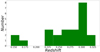 |
Fig. 1. Redshift histogram of the 24 GPs in our sample. |
Name, position, redshift, and observation data.
From a first inspection of the data cubes, our GPs appear compact and almost point-like except for a few of them. In order to ensure that we can spatially resolve these galaxies, the FWHM of all the sources within the FoV has been measured in white light1. We checked the objects in the FoV that are stars according to SDSS DR16 (Ahumada et al. 2020). Then, we defined the stellar-like FWHM (FWHM⋆) as the median stellar FWHM, and, in case there are no SDSS stars in the FoV, we defined the FWHM⋆ as the FWHM of the least extended object within the FoV. We considered a GP to be extended if its FWHM (FWHMGP) follows this condition:

After applying this criterion, 12 GPs are considered to be extended out of 24. The FWHM⋆ and the FWHMGP along with the number of stars in the FoV can be seen in Table 2.
Extension of stellar-like sources and GPs.
The previous analysis allows us to determine which galaxies present a resolved core. Nevertheless, thanks to the very high VLT/MUSE sensitivity, we can also check the extended nature of these galaxies in low surface brightness. In order to prove it, an analogous analysis of the previous one is realized but using instead the full width at  of the maximum (
 ) and the full width at
  of the maximum (
 ). These parameters trace the extension of the objects at lower surface brightness. We consider that a GP is extended in the low surface brightness regions if one of the following conditions is satisfied:
After applying this criterion, 11 GPs are considered to be resolved in the low surface brightness regions out of 24. The  and
and  of the stellar-like sources and the GPs can be seen in Table 2.
Due to the redshift distribution in our sample of GPs, the spectral coverage of MUSE provides us with most of the emission lines in the optical wavelengths. In particular, for all GPs we have all the emission lines from Hδ to [S II]λ6731 Å. For 13 of them we can reach the [O II]λ3727 Å line.
Rayleigh scattering of the atmosphere would spread the light from a source depending on wavelength, and the extension of the emission line maps at substantially different wavelengths (e.g., Hα vs. Hβ and [O III]5007 Å vs. [O II]3727 Å, 3729 Å) might be affected. Aiming to correct by this effect, a detailed analysis was performed sampling the FWHM for all the sources (within the FoV of each GP) along the entire wavelength range, showing that blue images in the cubes have a lower spatial resolution than red images. We derived a decrease in the FWHM (as wavelength increases) of the sources ranging from 2.25 × 10⁻⁵ arcsec Å−1 to 1.15 × 10⁻⁴ arcsec Å−1. This information allowed us to apply the appropriate gaussian kernel to red images to effectively compare them with the blue images.
The MUSE pipeline corrects the data for the effect of atmospheric differential refraction. As a sanity check, we measured the center of all the objects detected in the cubes in the spectral ranges of [4900, 5100] Å and [8950, 9150] Å, finding a mean difference of only 0.07″ (Weilbacher et al. 2020).
2.2. SDSS spectra
We retrieved SDSS-DR16 integrated spectra for all the GPs (Ahumada et al. 2020). The diameter of the SDSS fiber is 3″. The wavelength coverage is 3800−9200 Å. The spectral resolution is 1500 at 3800 Å and 2500 at 9000 Å. The pixel spacing log wavelength is 10−4 dex and the exposure times are in the range of 2800 s−8500 s.
3. Flux measurements and spatially resolved structure
In this section, we describe the methodology followed to measure the flux of the emission lines in the galaxies. Additionally, we present the spatially resolved maps generated from the spaxel-to-spaxel measurements of fluxes and continuum along with the so-called BPT diagrams (Baldwin et al. 1981; Kewley et al. 2006).
3.1. Emission line and continuum maps
For each spaxel, all the emission lines were fit to a gaussian profile, which gives us the flux of each line. The errors in the fluxes were calculated using the bootstrap method (Efron & Tibshirani 1985). We combined the line fluxes with the position of the fibers in the sky to create the maps of emission lines presented in this paper.
As an example, the emission line maps of the galaxy GP06 are shown in Fig. 2. Among the galaxy sample, GP06 is the one that presents the most complex structure in these maps, where even in dim lines like [S II]6716 Å and [S II]6731 Å a small bump is seen in the south-western position with respect to the central burst. Furthermore, this galaxy presents the brightest nebular HeII4686 Å emission (also detected in GP20 and GP15) in our sample. This line indicates the presence of very high energy photons (E > 4 Ry) that strongly ionize the gas and raise the electron temperature (e.g., Kehrig et al. 2015). The emission line maps corresponding to the rest of the galaxies are presented in Appendix A. All emission lines in our set of GPs peak in the center of the galaxy. This indicates that the total brightness of the galaxies is dominated by a compact region where the ionization sources are present. This region is slightly resolved for only a few GPs (e.g., GP13; see Fig. A.13) The only four GPs that present non-circular symmetry in the low surface brightness regions are GP06, GP13, GP07, and marginally GP01 (see Figs. 2, A.1, A.7, and A.13). The most extended structures in the maps are the ones corresponding to the [O III]5007 Å line and, in lesser terms, to the Hα line. The high intensity of these lines allows us to trace the low surface brightness regions corresponding to the ionized gas in the outer parts of the galaxies. Dimmer emission lines (e.g., Hβ, [N II]6584 Å, [S II]6716 Å, [S II]6731 Å, [O I]6300 Å, and [O III]4363 Å) present less extension and more circular symmetry.
 |
Fig. 2. GP06 emission line maps. The black line in the bottom left corresponds to a distance of 10 kpc. The circle in the bottom right is the representation of the seeing. The peak in the Hα emission is represented by the black point in the middle. The green and black contour represents the 3σsky level of the continuum map corresponding to the same galaxy. All maps presented in this work have the previously mentioned features except for the continuum maps, which do not present the continuum contour. Black contours are regions with different signal = k × σsky levels (with k = 10, 100), and all spaxels represented in all maps are above 3σsky. The red contour indicates the FWHM of the map. The same contours are shown in each emission line map and continuum map in this study. |
To make the continuum maps, we selected a rest frame spectral range common to all galaxies to integrate the continuum. Since each galaxy has a different redshift, they present a different rest frame spectral range. So, we can take the intersection of all these to define our rest frame spectral range for defining the continuum. This is indeed between 4154 Å and 7026 Å, very close to the spectral range of the human eye. To make these maps we removed the lines in the spectrum of each spaxel. Then, we integrated the spectrum in our selected rest-frame spectral range. In Fig. 3, we present the continuum map corresponding to GP06. The continuum maps of all GPs are in Fig. C.1. As seen in these maps, all galaxies present a richer structure than in the emission line maps. One of the reasons behind this is the fact that we are collecting more light, since the rest frame spectral range is 2872 Å wide. In order to collect the same amount of light from a line, its EW must be similar, while their values are up to 2000 Å. Continuum maps show bumps attached to the central part of the galaxy in many cases (e.g., GP03, GO06, GP13, GP15). Such disturbed morphologies of the continuum could indicate a spread in the underlying stellar population due to recent mergers (Lofthouse et al. 2017).
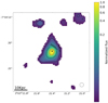 |
Fig. 3. Continuum map of GP06. Integration is done between 4154 Å and 7026 in rest frame. |
Even if we are collecting more light in the continuum than in the emission lines, the galaxies show a more compact appearance in the continuum maps than the [O III]5007 emission line maps. This possibly indicates that we are tracing the ionized gas in the outer parts of the galaxies, since the underlying stellar population is less extended than the ionized gas. In particular, GP06 presents two regions in the north east and north west (with respect to the Hα peak), where the [O III]5007 emission line extends much further (up to 10 kpc) than the continuum (Figs. 2 and 3). In these galactic regions, there is almost no extinction (Hα/Hβ ∼ 2.86), and the gas has higher excitation (log([O III]λ5007/Hβ)∼0.7) in comparison to the other outer regions where log([O III]λ5007/Hβ)∼0.45 (see Sect. 3, Figs. 4 and 6). Similar results were found for the galaxy SBS 0335–052E where [O III]5007 and Hα filaments with low Hα/Hβ ratio were discovered (Herenz et al. 2023). These observations point to the fact that these regions can be channels where LyC photons can escape. In particular, for the case of GP06 it is found that this galaxy presents an optically thick, neutral outflow along the line of sight (LOS; Jaskot & Oey 2014), making the escape of high-energy photons difficult in this particular direction (with fesc(Lyα) = 0.05 as found in Jaskot et al. 2017). However, this galaxy displays one of the highest ratios of [O III] to [O II] in this study ([O III]/[O II] = 6.56). This suggests that there could be potential escape paths for ionizing photons in other directions (Izotov et al. 2022).
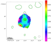 |
Fig. 4. Hα/Hβ map of GP06 before reddening correction. |
3.2. Emission line ratio maps
Here, we present maps of some of the relevant line ratios to study the ionization structure of the gas in our set of GPs. These line ratios are corrected for reddening using the corresponding c(Hβ) for each spaxel; c(Hβ) was computed from the ratio of the measured-to-theoretical Hα/Hβ assuming the reddening law of Cardelli et al. (1989), and case B recombination with the electron temperature Te = 104 K and electron density ne = 100 cm−3, which give an intrinsic value of Hα/Hβ = 2.86. In Fig. 4, we show the uncorrected Hα/Hβ map for GP06. The Hα/Hβ map is a tracer of dusty regions, and the zones with higher extinction are likely to present dust that acts like a wall for high-energy photons (Weingartner et al. 2006). Hence, if there is an escape of LyC photons, the preferred direction would be the one that presents lower extinction. The emission line ratio maps for all GPs are provided in Appendix B.
The MUSE spectral coverage allows us to observe the [O II]λλ3727,3729 lines for 13 of our GPs due to their redshifts, so we can analyze the map of the [O III]λ5007/[O II]λλ3727,3729 ([O III]/[O II]) line ratio (see Appendix ), which traces the ionization of the gas, in these galaxies. As an example, in Fig. 5 we show the map of this ratio for GP13, which is the most extended galaxy in our sample. High values of [O III]/[O II] trace galactic regions with high ionization. These regions tend to be near the center of the galaxy where the Hα peaks and the main ionizing sources are also located. The highest values of [O III]/[O II] are found in GP22 and GP15 (see Figs. B.15 and B.22), reaching a value of 6.5.
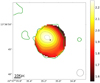 |
Fig. 5. [O III]5007/([O II]3727 + [O II]3729) map of GP13. |
The ratios used in the BPT diagrams are [O III]λ5007/Hβ ([O III]/Hβ), [N II]λ6584/Hα ([N II]/Hα), [S II]λλ6716,6731/Hα ([S II]/Hα), and [O I]λ6300/Hα ([O I]/Hα). Examples of maps corresponding to these line ratios are displayed in Fig. 6.
 |
Fig. 6. BPT maps corresponding to GP06. |
High values of [O III]/Hβ correspond to the areas of ionized gas with relatively higher excitation. The [O III]/Hβ maps do not show significant spatial variations (with a maximum difference of < 0.1 dex) for any of the GPs except for GP06, indicating low spatial gradients in gas excitation. For this galaxy, the spatial variation of [O III]/Hβ goes up to 0.4 dex, with a maximum very close to the center of Hα emission (see Fig. 6). The outer zones of this galaxy with lower [O III]/Hβ ([O III]/Hβ ∼ 0.45) present high extinction (Hα/Hβ ∼ 4.25; see north, south-east and south-west regions in Figs. 4 and 6). As the photons reach the outer parts from the central starburst, they tend to be absorbed, so this radiation becomes softer as it goes through dusty regions. GP20 presents the highest value of [O III]/Hβ, reaching log([O III]/Hβ) = 0.91 (see Fig. B.20). This galaxy also exhibits the most prominent emission lines (see Table ).
Low values of [N II]/Hα in the maps indicate regions with higher gas excitation and trace low metallicity zones (Pettini & Pagel 2004). The [N II]/Hα maps do not present much spatial variance, with a maximum difference of 0.14 dex for GP08 (see Fig. B.8). Indicating low spatial variations in gas excitation and metallicity. The lowest values in [N II]/Hα are found in GP06, GP15, and GP20 (see Figs. B.6, B.15 and B.20). These three galaxies are also the ones that show nebular HeII4686 Å emission, which indicates the presence of hard ionizing sources.
[S II]/Hα maps trace the opacity of the column of gas (i.e., gas in the line of sight in each spaxel; Pellegrini et al. 2012). [O I]/Hα peaks in the ionization front (edge of ionization-bounded regions). Low values on both coefficients indicate thin columns of gas (and as well, high gas excitation) where LyC photons are likely to escape (Paswan et al. 2022). We can see that most GPs present a blister-type morphology, which is characterized by an optically thin galactic center, and as we go to the outer parts (around 5−10 kpc) the medium tends to become optically thick (see Appendix ). An extremely low [S II]/Hα value could indicate a hole from which photons can escape (Wang et al. 2021), being GP06, GP15, and GP20 the most extreme cases again (see Figs. B.6, B.15, and B.20).
The last two maps presented here are [S II]λ6716/[S II]λ6731 and [O III]λ4363/[O III]λ5007. Examples of maps corresponding to these line ratios are displayed in Fig. 7. These emission line ratios give us information about the electron density and electron temperature, respectively (e.g., Pérez-Montero 2017). Higher [S II]λ6716/[S II]λ6731 values correspond to lower electron densities, whereas higher [O III]λ4363/[O III]λ5007 values correspond to higher electron temperatures. The maps corresponding to these two line ratios do not present clear radial variances, while they show a wide variety of morphologies despite the low spatial extension of these dim lines (see Appendix ). In the particular case of GP06, the values of the [S II]λ6716/[S II]λ6731 ratio are higher where the gas shows lower excitation (as traced by [O III]/Hβ and [S II]/Hα) and higher extinction regions (traced by Hα/Hβ). This indicates that for this galaxy the electron density tends to a decrease in the regions with higher dust content and lower gas excitation. Moreover, the highest values for [O III]λ4363/[O III]λ5007 (line-ratio indicator of the electron temperature) are found in the galaxies with HeII4686 Å emission (see Figs. B.6, B.15 and B.20), which reinforces the existence of a harder ionizing radiation field in these objects (see, e.g., Kehrig et al. 2016).
 |
Fig. 7. Maps corresponding to GP06. |
We present the radial profiles of the emission line ratios previously mentioned. By plotting the emission line ratio as a function of radial distance, we effectively visualize the radial variations in the line ratios across the galaxy. This representation facilitates the identification of radial trends and provides a comprehensive understanding of how these line ratios evolve as we move away from the galactic center.
To obtain the radial profiles, we utilized a technique that integrates circular crowns centered around the peak of Hα emission. The code calculates the average value of the emission line ratio within each crown and plots it against the radial distance from the center. The radial profiles of Hα/Hβ are shown in Fig. 8. The rest of the radial profiles are in Appendix D.
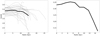 |
Fig. 8. Radial profile of Hα/Hβ. The left image shows the profiles of all GPs with available information about the lines in gray. In black it is represented the mean of all galaxies and extends up to a radius where only 30% of the galaxies present values at larger radii. On the right is a zoomed-in image of the mean profile. The same display applies to all line ratios presented in the appendix. |
One notable observation is that the overall radial tendencies of the emission line ratio profiles are similar across the entire set of galaxies. However, there are substantial variations in the absolute values of the ratios between different galaxies, typically on the order of 0.5 dex. In contrast, within each individual galaxy, the radial change in the emission line ratios is relatively small, typically less than 0.1 dex. This small radial variation within each galaxy could potentially be attributed to the low spatial resolution of our observations.
Despite the low radial change within each galaxy, the mean radial profiles of all galaxies present clear tendencies for the various emission line ratios studied. These profiles provide valuable insights into the ionization state within the galaxies.
We observe a consistent decrease in the [O III]/[O II] and [O III]5007/Hβ ratios and an increasing trend in the [S II]/Hα, [O I]/Hα, and [N II]/Hα ratios as we move away from the galactic center. This implies that the highest level of ionization and density-bounded tracers are predominantly concentrated in the central regions of the galaxies. Still, the mean variation in the [O III]5007/Hβ and [N II]/Hα ratios are really low (0.03 dex and 0.015 dex, respectively), indicating that the radial changes in these emission line ratios are nearly imperceptible.
Furthermore, the radial tendency in the Hα/Hβ ratio indicates a decreasing trend as we move toward the outer parts of the galaxies. This suggests a relatively higher level of extinction or enhanced dust attenuation toward the central regions, resulting in a higher Hα/Hβ ratio compared to the outskirts.
In contrast, the radial changes in the [S II]λ6716/[S II]λ6731 and [O III]λ4363/[O III]λ5007 ratios are small (on the order of the previously mentioned [N II]/Hα ratio) and do not exhibit a clear radial trend. These ratios may be less sensitive to radial variations or they are influenced by other factors such as excitation conditions or observational uncertainties.
Overall, the mean radial profiles of the emission line ratios consistently reveal the spatial variations in the ionization state within the galaxies. The observed trends support the notion that the central regions of the galaxies exhibit higher ionization levels and greater density-bounded tracers, while the outer parts experience lower ionization conditions.
3.3. BPT diagrams
The BPT diagrams for all our GPs are shown in Fig. 9 on a spaxel-by-spaxel basis; there, we can see the line ratios [O III]5007/Hβ versus [N II]/Hα, [S II]/Hα, and [O I]/Hα plotted. Small dots correspond to measurements from individual spaxels for each galaxy. Big green dots show the line ratios derived from the integrated spectra (see Sect. 4), these values are shown in Table F.2.
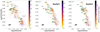 |
Fig. 9. BPT diagram. Small dots in the color scale (from yellow to dark purple) correspond to spaxels in each galaxy. Big green dots correspond to the integrated spectra of the galaxy. Next to the green dots we can see the name of each galaxy. The color of the small dots corresponds to the distance to the center of the galaxy. The closer to the center the more yellow they are, and farther away from the center they become darker. The lines that delimitate each region are taken from Kewley et al. (2001) and Kauffmann et al. (2003). |
Overall, our GPs fall in the general locus of SF objects according to the spectral classification scheme proposed by Baldwin et al. (1981) and Kewley et al. (2006). This suggests that photoionization from hot massive stars is the dominant excitation mechanism within these galaxies. In particular, GPs are located in the top left part of the diagram where the most extreme galaxies reside (i.e., lower metallicity and higher excitation of the ionized gas). Previous studies confirm this trend for GPs (e.g., Cardamone et al. 2009; Jaskot & Oey 2013). Furthermore, GPs share with EELGs the same region in the [O III]5007/Hβ versus [N II]/Hα diagram as Pérez-Montero et al. (2021) showed.
Furthermore, there is no presence of the Fe[X]λ6374 Å line in any GP. This line is a tracer of black hole (BH) activity. Luminosities of this line on the order of 1036 − 1039 erg s−1 correspond to the presence of BHs with a mass of ∼105 M⊙ (Molina et al. 2021). Nevertheless, due to the distance of GPs, it is not possible to measure lines with luminosities ≫1040 erg s−1. Such limitations lead us to conclude that GPs do not present actively accreting BHs with a mass ≫105 M⊙.
In addition, we used a method for estimating BH masses involving the use of a BH mass – stellar mass relation – which states that it is nearly independent of redshift (Shankar et al. 2020). Nevertheless, our range of stellar masses, which covers from 108.3 M⊙ to 1010 M⊙ in the low end, is well below the predictive capacity of the relation. Thus, we are only using it for the GPs with higher masses (∼1010 M⊙); for these galaxies, the expected BH mass is no greater than 106.7 M⊙.
This estimation is clearly above 105 M⊙ solar masses, which suggests that if these galaxies do contain BHs, these BHs have a low mass compared to the total stellar mass of the galaxy. It is important to note, however, that with the use of the Shankar et al. (2020) relation we cannot accurately predict BH masses in galaxies with M⊙ < 109.8. That is why it is so difficult to retrieve any information from the BHs in the low stellar mass GPs. Further observations and analysis are needed to confirm the presence and measure the exact masses of any BHs in these galaxies.
In the BPT diagrams, the distance from the center of the galaxy as a parameter is also represented. We can see a common tendency for all galaxies. As we go closer to the center of the galaxy, it shows a higher [O III]5007/Hβ ratio (i.e., higher excitation close to the center) and lower [S II]/Hα and [O I]/Hα ratios (i.e., the center of the galaxies are optically thinner, and neutral oxygen is more abundant in the outer part). Regarding the [N II]/Hα ratio, it is almost independent of distance, possibly indicating that metallicity gradients are low. All these results are in agreement with the ones presented in the previous section (Sect. 3.2).
4. Properties of GPs from integrated spectra
We also took advantage of our IFS data to produce the 1D spectra of selected galaxy regions. To do so, for each GP, we added the flux in all spaxels for which the Hα flux measurements present a signal-to-sigma sky ratio greater than three (S/σsky > 3). As an example, the integrated spectrum of the galaxy GP06 can be seen in Fig. 10. The integrated spectra of all GPs are shown in Fig. E.1. We did not find in any of the spectra features of WR stars.
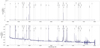 |
Fig. 10. Integrated spectrum of GP06. The bottom image is a zoomed-in view of the y-scale of the top image. |
We used the integrated spectrum of each GP to identify and measure the most relevant emission lines. The same procedure as the one used in Sect. was used to calculate emission line fluxes, errors, and extinction correction. Appendix lists all the data of the emission lines. To check the wellness in the flux measurement, the MUSE integrated spectra and the SDSS spectra were compared, retrieving that, on average, the ratio between the fluxes per line is 1.003 ± 0.038. Additionally, the spectral coverage of SDSS extends to shorter wavelengths than MUSE, enabling us to obtain the flux of the [O II] line for the 11 GPs that do not present this line in MUSE. We used the MUSE fluxes in all other cases.
4.1. SFR
By means of the Kennicutt relation (Kennicutt 1998), we derived the SFR through the Hα luminosity (Hα luminosity was retrieved using luminosity distances from the UCLA cosmology calculator2) in the following way:

Most of the stellar masses (M⋆) were reproduced from Izotov et al. (2011); nevertheless, Izotov et al. (2011) did not calculate the mass for all the galaxies in our sample, and so the Cardamone et al. (2009) value was used instead. Izotov et al. (2011) recalculated the masses of the GPs and obtained systematically lower values. Their values are lower because in fitting the SED, they subtracted the contribution from gaseous continuum emission. No errors were listed in the original studies. The corresponding specific SFRs were derived as follows: sSFR = SFR/M⋆.
In Fig. 11, we display sSFR versus stellar mass. Here, GPs occupy a different region in the diagram than present-day galaxies (galaxies at z < 0.05; Catalán-Torrecilla et al. 2015). GPs have lower masses and much higher sSFRs. In fact, GPs share the same space in this diagram with high-redshift galaxies z = 1.1 − 4. The mass-doubling timescale of GPs is on average 2 dex lower than that of present-day galaxies, reaching down to ∼15 Myr for GP20, GP22, GP18, and GP15.
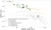 |
Fig. 11. Stellar mass versus sSFR. Green points are the GPs presented in this work, light green are GPs with HeII emission. The green star represents the median of the GPs, corresponding to a stellar mass of 2.6 × 10⁹ M⊙, an sSFR of 12 Gyr−1, and thus a mass-doubling timescale of 47 Myr. Black points represent a set of local galaxies (z < 0.03) from the Califa survey (Catalán-Torrecilla et al. 2015; Torrecilla15). The black star represents the median of this sample, it corresponds to a stellar mass of 3.2 × 10¹⁰ M⊙, a sSFR of 0.12 Gyr−1 and thus a mass-doubling timescale of 8.3 Gyr, which is on the order of the age of the Universe. We also show the sSFR-mass relation at a variety of redshifts from Tasca et al. (2015; dash-dot line, T15), Karim et al. (2011; dashed line, K11), and Whitaker et al. (2012; dotted line, W12). |
The depletion timescale, which indicates the starburst duration, is on the order of the mass-doubling timescale (which is the inverse of the sSFR) only if the mass of available hydrogen for creating new stars (MH II) is on the order of the M⋆. Nevertheless, if MH II > M⋆ the starburst duration is larger than the mass-doubling timescale. If we consider that MH II ≃ M⋆, this could indicate that GPs are short-lived events, since they will not be able to support such an incredibly high SFR for a long time. The mechanisms that would stop the SFR are mainly the exhaustion of the gas that fuels star formation and the stellar feedback via supernovae (Amorín et al. 2012). Observationally, we have very little information on whether GPs will immediately quench or not. However, if they continue forming stars, they would quite rapidly build stellar mass and increase the stellar luminosity in the blue, and the EW of [O III]5007 Å will decrease. Thus, they would no longer be selected as GPs, given the effective criterion of having high EW in [O III]5007 Å. Using this kind of argument one could state that they are the analogs of the early phases of galaxies that reionized the Universe.
The GP15 galaxy is identified as an LyC leaker exhibiting an escape fraction for LyC, fesc(LyC) = 0.08 (Izotov et al. 2016) and for Lyα, fesc(Lyα) = 0.51 (Jaskot et al. 2017). This aligns with the understanding that the most intense starburst events typically generate a higher quantity of ionizing photons. Furthermore, this galaxy present among the most extremes line ratios favoring escape of ionizing photons (high [O III]/[O II] and low [S II]/Hα and [N II]/Hα) see Table F.2.
4.2. Electron density, temperature, and abundances of the ionized gas
In this section, we discuss how we derived chemical abundances of the ionized gas and electron temperatures (Te) and densities (ne). The emission line [O III]4363 Å is essential to calculate electron temperature and hence abundances. There are six GPs (out of the 24 GPs analyzed in this work) in which this line can be detected (i.e., the line is above the three-sigma detection limit). For this subset of galaxies, we derived the Te values of [O III] using the [O III]λ4363/[O III]λ4959,5007 line ratio and the values of Te corresponding to [O II] from the empirical relation between [O II] and [O III] electron temperatures given by Campbell et al. (1986). We obtained the electron densities, from the [S II]λ6716/[S II]λ6731 line ratio. The oxygen ionic abundance ratios, O+/H+ and O2+/H+, were derived from the [O II]λ3727 and [O III]λλ4959,5007 lines, respectively, using the corresponding electron temperatures. The total oxygen abundance is assumed to be O/H = O+/H+ + O2+/H+. The nitrogen ionic abundance ratio, N+/H+, was calculated using the [N II]λ6584 emission line and assuming Te [N II] ∼ Te [O II]; the N/O abundance ratio was computed under the assumption that N/O = N+/O+, based on the similarity of the ionization potentials of the ions involved. All this was computed by implementing the Pyneb code (Luridiana et al. 2015). We calculated the final errors in the derived quantities by error propagation and taking into account errors in flux measurements. Furthermore, for the subset of galaxies that do not present the [O III]4363 Å line, we used the HII-CHI-Mistry code (Pérez-Montero 2014), which calculates oxygen and nitrogen over oxygen abundances (and errors) without this line. The values corresponding to all these gas properties are shown in Table F.2.
In Fig. 12, we can see the electron density, electron temperature, and metallicity for the six GPs with the [O III]4363 Å line measured. The same properties are also represented for 35 galaxies selected from the NASA-Sloan Atlas3 with W(λ5007) > 1000 Å and 37 galaxies from the COS Legacy Archive Spectroscopic SurveY (Berg et al. 2022) galaxies, which are the closest local analogs (z < 0.18) of high-redshift galaxies in the epoch of reionization. The derivation of gas parameters in these galaxies was done by Peng (2021). The metallicity of our set of GPs is low and in agreement with previous results (i.e., 12 + log(O/H) = 7.6 − 8.4; e.g., Amorín et al. 2010). For this subset of GPs with [O III]4363 Å emission, the electron temperature ranges from 11 500 K to 15 500 K and the electron density ranges from 30 cm−3 to 400 cm−3.
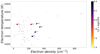 |
Fig. 12. Electron density, electron temperature, and metallicity representation. Big labeled dots correspond to the six GPs where the direct method can be well applied. The rest of the small dots correspond to all galaxies selected from the NASA-Sloan Atlas with W(λ5007) > 1000 Å and 37 COS Legacy Archive Spectroscopic SurveY galaxies. |
Figures 13–15 display the oxygen abundance versus stellar mass, nitrogen over oxygen versus stellar mass, and nitrogen over oxygen versus oxygen abundance, respectively. A comparison is made between ∼200 000 star-forming galaxies (SFGs) from SDSS (Duarte Puertas et al. 2022) and the GPs. For a given stellar mass, GPs show lower oxygen abundances than the bulk of the SDSS galaxies. This is in accordance with the result from Amorín et al. (2010), where GPs follow a relation between mass and metallicity parallel to the one defined by the SDSS SFGs, but it is offset by ∼0.3 dex to lower metallicities. The nitrogen over oxygen (N/O) ratio (Fig. 14) of GPs follows the tendency of SDSS galaxies, except for the low-mass end, where GPs present a higher N/O (see GP22, GP18 and GP20 in Fig. 14). This ratio ranges from log(N/O) = − 1.5, −0.85.
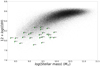 |
Fig. 13. Oxygen abundance versus stellar mass. GPs are the green points. Black points correspond to ∼200 000 galaxies from Duarte Puertas et al. (2022). |
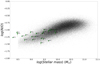 |
Fig. 14. Nitrogen over oxygen versus stellar mass. GPs are the green points. Black points correspond to ∼200 000 galaxies from Duarte Puertas et al. (2022). |
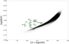 |
Fig. 15. Nitrogen over oxygen versus oxygen abundance. GPs are the green points. Black points correspond to ∼200 000 galaxies from Duarte Puertas et al. (2022). |
Despite the lack of metals in GP galaxies, the metal ratio (N/O) is mostly conserved. One scenario that can explain this would be a massive and recent inflow of metal-poor gas (basically neutral hydrogen clouds) from the HI halo/reservoir of the galaxy. This accretion could dilute the O/H keeping the N/O unaltered (Köppen & Hensler 2005). The fact that their N/O is in most cases the expected for the stellar masses of these galaxies supports this scenario (Amorín et al. 2010).
The proposed scenario of a massive inflow of pristine gas that both sustains low metallicity and increases the SFR is plausible. However, this raises a complex issue regarding the presence of such a process at low redshifts. The origins of this unenriched gas remain an area of inquiry. Nonetheless, empirical data provides insight with evidence from extremely metal-poor galaxies proximal to us (z = 0.03) that exhibit substantial amounts of neutral hydrogen, resembling a halo (e.g., Lequeux & Viallefond 1980; Herenz et al. 2023). This suggests that similar circumstances could exist for GPs, thereby supporting the proposed scenario.
Chemical evolution model predictions (e.g., Mollá et al. 2006; Vincenzo et al. 2016) suggest that the transition between primary and secondary N dominance in the N/O versus O/H plane depends on the SF history, particularly on the star formation efficiency (SFE). A “bursty” galaxy, that is, one having experienced a very recent starburst, will see a quicker increase in N/O than a galaxy with a smoother and longer SF history. Another factor that could elevate the N/O at low metallicity is the initial mass function (IMF), where a higher fraction of massive stars could enhance primary N production at low metallicity. However, we observe that the N/O – stellar mass relation generally holds. For galaxies deviating from this relation (see GP22, GP18, and GP20 in Fig. 14), adjusting the IMF could be a viable solution.
5. Summary and conclusions
We have presented physical and chemical properties of 24 GPs using MUSE/VLT data cubes. These galaxies are one of the best local analogs of high-redshift galaxies. Thus, their study is fundamental in order to understand the very first epoch of the formation and assembling of galaxies, and in particular the reionization.
For our set of GPs, we wanted to confirm the spatial extension of these sources. To do so, a study regarding the extension of all the sources within the FoV of the MUSE data cube was carried out. We established a criterion to determine whether a GP is resolved based on the comparison between the FWHM,  , and
, and  of a stellar-like object and the GP itself. Retrieving seven spatially extended GPs in the core and the low surface brightness region, five GPs extended in the core, and four GPs extended in the low surface brightness region (see Table ).
We compare the emission line maps and the continuum maps. The only four emission line maps with no circular symmetry are the ones corresponding to GP06, GP07, GP13, and, marginally, GP01. Continuum maps present a much richer structure for all GPs that are proxies for the stellar underlying population. [O III]5007 maps are the most extended ones, tracing the low surface brightness regions of ionized gas.
Regarding the ionization structure, Hα/Hβ maps trace dusty regions and zones with low extinction where photons can travel without being absorbed; these maps present very different morphologies for the different GPs. The ionization parameter (as traced by [O III]/[O II]) tends to peak in the center of the galaxies, indicating that the highest ionization is near the star-forming region. GP20, GP06, GP15, and GP22 present the strongest ionization (see Table and Figs. B.15 and B.22). The [O III]/Hβ, [N II]/Hα, [S II]/Hα, and [O I]/Hα ratios are studied in maps and in the BPT diagrams. These indicate a tendency for higher excitation of the gas in the center of the galaxy (i.e., higher ratios of [O III]/Hβ and lower ratios of [S II]/Hα and [O I]/Hα close to the Hα peak). Still, the [O III]/Hβ and [N II]/Hα ratios do not present much spatial variation (with a maximum difference of 0.14 dex in all GPs, except for GP06 reaching over 0.4 dex), indicating uniformity in the gas excitation and metallicity. [S II]/Hα and [O I]/Hα trace the boundaries of the ionized gas, and they present their lower values close to the center of the galaxies, suggesting a blister-type morphology (e.g., GP06, GP08, GP10, GP13, and GP23).
The BPT diagrams indicate hot massive stars are confirmed as the main source of ionizing photons. In particular, our GPs are located in the top left part of the diagram, where the most extreme galaxies reside (i.e., those with the lowest metallicity and highest excitation of the ionized gas). The absence of the [FeX]λ6374 in all the spectra discards BHs with masses ≫105 M⊙ contributing to ionizing the gas.
We also produced the integrated spectrum of each GP by integrating the flux of a region defined by the Hα map. The SFRs derived from the luminosity of the Hα line indicate bursts of star-formation with mass-doubling timescales 2 dex lower than common star-forming galaxies. Our study of the ionized gas properties using emission lines indicates low gas metallicity (i.e., 12 + log(O/H) = 7.6 − 8.4), high electron temperatures ranging from 11 500 K to 15 500 K, and electron densities ranging from 30 cm−3 to 530 cm−3. The nitrogen over oxygen ratio versus stellar mass of the GPs (see Fig. 14) generally follows the tendency of SDSS galaxies and ranges between log(N/O) = − 1.5 and −0.85, whereas these are clearly above the SDSS sequence in the log(N/O) versus 12 + log(O/H) diagram (see Fig. 15), which possibly indicates the presence of an inflow of pristine gas into the galaxies.
We detected the nebular HeIIλ4686 line in the galaxies GP06, GP15 (this particular galaxy being a confirmed LyC leaker Izotov et al. 2016), and GP20, indicating the presence of very hard ionizing photons (E > 4 Ry). We checked that none of these GPs show WR features in their spectra, which suggests that WR stars are not the main HeII excitation contributors (e.g., Senchyna et al. 2017; Kehrig et al. 2015, 2018). We also note that two of these GPs present among the highest sSFR (> 8 × 10⁸ yr−1), suggesting that, besides a low metallicity, high sSFR can be a dominant factor to determine the HeII emitting nature of a galaxy (Kehrig et al. 2020; Pérez-Montero et al. 2020). A detailed analysis of the origin of the HeII ionization, which keeps challenging up-to-date stellar models (see e.g., Eldridge & Stanway 2022), is beyond the scope of this work and will be investigated in future work.
Acknowledgments
We thank the referee for their constructive comments. Author Antonio Arroyo Polonio acknowledges financial support from the grant CEX2021-001131-S funded by MCIN/AEI/10.13039/501100011033. R.A. acknowledges support from ANID FONDECYT Regular Grant 1202007.
References
- Ahumada, R., Prieto, C. A., Almeida, A., et al. 2020, ApJS, 249, 3 [Google Scholar]
- Amorín, R. O., Pérez-Montero, E., & Vílchez, J. 2010, ApJ, 715, L128 [CrossRef] [Google Scholar]
- Amorín, R., Vílchez, J. M., Hägele, G. F., et al. 2012, ApJ, 754, L22 [CrossRef] [Google Scholar]
- Bacon, R., Accardo, M., Adjali, L., et al. 2010, Proc. SPIE, 7735, 773508 [Google Scholar]
- Bae, H.-J., Woo, J.-H., Karouzos, M., et al. 2017, ApJ, 837, 91 [NASA ADS] [CrossRef] [Google Scholar]
- Baldwin, J. A., Phillips, M. M., & Terlevich, R. 1981, PASP, 93, 5 [Google Scholar]
- Berg, D. A., James, B. L., King, T., et al. 2022, ApJS, 261, 31 [NASA ADS] [CrossRef] [Google Scholar]
- Breda, I., Vilchez, J. M., Papaderos, P., et al. 2022, A&A, 663, A29 [NASA ADS] [CrossRef] [EDP Sciences] [Google Scholar]
- Cairós, L., Caon, N., Zurita, C., et al. 2009, A&A, 507, 1291 [NASA ADS] [CrossRef] [EDP Sciences] [Google Scholar]
- Campbell, A., Terlevich, R., & Melnick, J. 1986, MNRAS, 223, 811 [NASA ADS] [CrossRef] [Google Scholar]
- Cardamone, C., Schawinski, K., Sarzi, M., et al. 2009, MNRAS, 399, 1191 [NASA ADS] [CrossRef] [Google Scholar]
- Cardelli, J. A., Clayton, G. C., & Mathis, J. S. 1989, ApJ, 345, 245 [Google Scholar]
- Catalán-Torrecilla, C., De Paz, A. G., Castillo-Morales, A., et al. 2015, A&A, 584, A87 [NASA ADS] [CrossRef] [EDP Sciences] [Google Scholar]
- Chen, Z., Stark, D. P., Endsley, R., et al. 2023, MNRAS, 518, 5607 [Google Scholar]
- Curtis-Lake, E., Carniani, S., Cameron, A., et al. 2023, Nat. Astron., 7, 622 [NASA ADS] [CrossRef] [Google Scholar]
- Duarte Puertas, S., Vilchez, J. M., Iglesias-Páramo, J., et al. 2022, A&A, 666, A186 [NASA ADS] [CrossRef] [EDP Sciences] [Google Scholar]
- Efron, B., & Tibshirani, R. 1985, Behaviormetrika, 12, 1 [CrossRef] [Google Scholar]
- Eldridge, J. J., & Stanway, E. R. 2022, ARA&A, 60, 455 [NASA ADS] [CrossRef] [Google Scholar]
- Hayes, M. J., Runnholm, A., Scarlata, C., Gronke, M., & Rivera-Thorsen, T. E. 2023, MNRAS, 520, 5903 [NASA ADS] [CrossRef] [Google Scholar]
- Henry, A., Berg, D. A., Scarlata, C., Verhamme, A., & Erb, D. 2018, ApJ, 855, 96 [Google Scholar]
- Herenz, E. C., Hayes, M., Papaderos, P., et al. 2017, A&A, 606, L11 [NASA ADS] [CrossRef] [EDP Sciences] [Google Scholar]
- Herenz, E. C., Inoue, J., Salas, H., et al. 2023, A&A, 670, A121 [NASA ADS] [CrossRef] [EDP Sciences] [Google Scholar]
- Iglesias-Páramo, J., Arroyo, A., Kehrig, C., et al. 2022, A&A, 665, A95 [NASA ADS] [CrossRef] [EDP Sciences] [Google Scholar]
- Izotov, Y. I., Guseva, N. G., & Thuan, T. X. 2011, ApJ, 728, 161 [NASA ADS] [CrossRef] [Google Scholar]
- Izotov, Y., Schaerer, D., Thuan, T., et al. 2016, MNRAS, 461, 3683 [CrossRef] [Google Scholar]
- Izotov, Y., Chisholm, J., Worseck, G., et al. 2022, MNRAS, 515, 2864 [NASA ADS] [CrossRef] [Google Scholar]
- James, B., Tsamis, Y., & Barlow, M. 2010, MNRAS, 401, 759 [NASA ADS] [CrossRef] [Google Scholar]
- Jaskot, A., & Oey, M. 2013, ApJ, 766, 91 [NASA ADS] [CrossRef] [Google Scholar]
- Jaskot, A., & Oey, M. 2014, ApJ, 791, L19 [CrossRef] [Google Scholar]
- Jaskot, A. E., Oey, M., Scarlata, C., & Dowd, T. 2017, ApJ, 851, L9 [NASA ADS] [CrossRef] [Google Scholar]
- Karim, A., Schinnerer, E., Martínez-Sansigre, A., et al. 2011, ApJ, 730, 61 [Google Scholar]
- Kauffmann, G., Heckman, T. M., Tremonti, C., et al. 2003, MNRAS, 346, 1055 [Google Scholar]
- Kehrig, C., Vílchez, J., Sánchez, S., et al. 2008, A&A, 477, 813 [NASA ADS] [CrossRef] [EDP Sciences] [Google Scholar]
- Kehrig, C., Vílchez, J., Pérez-Montero, E., et al. 2015, ApJ, 801, L28 [NASA ADS] [CrossRef] [Google Scholar]
- Kehrig, C., Vílchez, J., Pérez-Montero, E., et al. 2016, MNRAS, 459, 2992 [NASA ADS] [CrossRef] [Google Scholar]
- Kehrig, C., Vílchez, J., Guerrero, M. A., et al. 2018, MNRAS, 480, 1081 [NASA ADS] [Google Scholar]
- Kehrig, C., Iglesias-Páramo, J., Vílchez, J., et al. 2020, MNRAS, 498, 1638 [NASA ADS] [CrossRef] [Google Scholar]
- Kennicutt, R. C., Jr. 1998, ApJ, 498, 541 [Google Scholar]
- Kewley, L. J., Dopita, M. A., Sutherland, R. S., Heisler, C. A., & Trevena, J. 2001, ApJ, 556, 121 [Google Scholar]
- Kewley, L. J., Groves, B., Kauffmann, G., & Heckman, T. 2006, MNRAS, 372, 961 [Google Scholar]
- Kim, K., Malhotra, S., Rhoads, J. E., Butler, N. R., & Yang, H. 2020, ApJ, 893, 134 [NASA ADS] [CrossRef] [Google Scholar]
- Köppen, J., & Hensler, G. 2005, A&A, 434, 531 [NASA ADS] [CrossRef] [EDP Sciences] [Google Scholar]
- Laufman, L., Scarlata, C., Hayes, M., & Skillman, E. 2022, ApJ, 940, 31 [NASA ADS] [CrossRef] [Google Scholar]
- Lequeux, J., & Viallefond, F. 1980, A&A, 91, 269 [NASA ADS] [Google Scholar]
- Lintott, C. J., Schawinski, K., Slosar, A., et al. 2008, MNRAS, 389, 1179 [NASA ADS] [CrossRef] [Google Scholar]
- Lofthouse, E. K., Houghton, R. C., & Kaviraj, S. 2017, MNRAS, 471, 2311 [NASA ADS] [CrossRef] [Google Scholar]
- Lumbreras-Calle, A., López-Sanjuan, C., Sobral, D., et al. 2022, A&A, 668, A60 [NASA ADS] [CrossRef] [EDP Sciences] [Google Scholar]
- Luridiana, V., Morisset, C., & Shaw, R. A. 2015, A&A, 573, A42 [NASA ADS] [CrossRef] [EDP Sciences] [Google Scholar]
- McKinney, J. H., Jaskot, A. E., Oey, M., et al. 2019, ApJ, 874, 52 [NASA ADS] [CrossRef] [Google Scholar]
- Molina, M., Reines, A. E., Latimer, C. J., Baldassare, V., & Salehirad, S. 2021, ApJ, 922, 155 [NASA ADS] [CrossRef] [Google Scholar]
- Mollá, M., Vílchez, J., Gavilán, M., & Díaz, A. I. 2006, MNRAS, 372, 1069 [CrossRef] [Google Scholar]
- Monreal-Ibero, A., Relaño, M., Kehrig, C., et al. 2011, MNRAS, 413, 2242 [NASA ADS] [CrossRef] [Google Scholar]
- Naidu, R. P., Oesch, P. A., van Dokkum, P., et al. 2022, ApJ, 940, L14 [NASA ADS] [CrossRef] [Google Scholar]
- Papaderos, P., Gomes, J., Vílchez, J., et al. 2013, A&A, 555, L1 [NASA ADS] [CrossRef] [EDP Sciences] [Google Scholar]
- Paswan, A., Saha, K., Leitherer, C., & Schaerer, D. 2022, ApJ, 924, 47 [NASA ADS] [CrossRef] [Google Scholar]
- Pellegrini, E. W., Oey, M. S., Winkler, P. F., et al. 2012, ApJ, 755, 40 [NASA ADS] [CrossRef] [Google Scholar]
- Peng, Z. 2021, PhD Thesis, University of California, USA [Google Scholar]
- Pérez-Montero, E. 2014, MNRAS, 441, 2663 [CrossRef] [Google Scholar]
- Pérez-Montero, E. 2017, PASP, 129, 043001 [CrossRef] [Google Scholar]
- Pérez-Montero, E., Kehrig, C., Vílchez, J., et al. 2020, A&A, 643, A80 [NASA ADS] [CrossRef] [EDP Sciences] [Google Scholar]
- Pérez-Montero, E., Amorín, R., Sánchez Almeida, J., et al. 2021, MNRAS, 504, 1237 [CrossRef] [Google Scholar]
- Pettini, M., & Pagel, B. E. 2004, MNRAS, 348, L59 [NASA ADS] [CrossRef] [Google Scholar]
- Rhoads, J. E., Wold, I. G. B., Harish, S., et al. 2023, ApJ, 942, L14 [NASA ADS] [CrossRef] [Google Scholar]
- Robertson, B., Tacchella, S., Johnson, B., et al. 2023, Nat. Astron., 7, 611 [NASA ADS] [CrossRef] [Google Scholar]
- Schaerer, D., Marques-Chaves, R., Barrufet, L., et al. 2022, A&A, 665, L4 [NASA ADS] [CrossRef] [EDP Sciences] [Google Scholar]
- Senchyna, P., Stark, D. P., Vidal-García, A., et al. 2017, MNRAS, 472, 2608 [NASA ADS] [CrossRef] [Google Scholar]
- Shankar, F., Weinberg, D. H., Marsden, C., et al. 2020, MNRAS, 493, 1500 [NASA ADS] [CrossRef] [Google Scholar]
- Tasca, L., Le Fèvre, O., Hathi, N., et al. 2015, A&A, 581, A54 [NASA ADS] [CrossRef] [EDP Sciences] [Google Scholar]
- Vincenzo, F., Belfiore, F., Maiolino, R., Matteucci, F., & Ventura, P. 2016, MNRAS, 458, 3466 [NASA ADS] [CrossRef] [Google Scholar]
- Wang, B., Heckman, T. M., Amorín, R., et al. 2021, ApJ, 916, 3 [NASA ADS] [CrossRef] [Google Scholar]
- Weilbacher, P. M., Palsa, R., Streicher, O., et al. 2020, A&A, 641, A28 [NASA ADS] [CrossRef] [EDP Sciences] [Google Scholar]
- Weingartner, J. C., Draine, B. T., & Barr, D. K. 2006, ApJ, 645, 1188 [NASA ADS] [CrossRef] [Google Scholar]
- Whitaker, K. E., Van Dokkum, P. G., Brammer, G., & Franx, M. 2012, ApJ, 754, L29 [NASA ADS] [CrossRef] [Google Scholar]
- Yang, H., Malhotra, S., Gronke, M., et al. 2016, ApJ, 820, 130 [NASA ADS] [CrossRef] [Google Scholar]
- Yang, H., Malhotra, S., Gronke, M., et al. 2017a, ApJ, 844, 171 [NASA ADS] [CrossRef] [Google Scholar]
- Yang, H., Malhotra, S., Rhoads, J. E., et al. 2017b, ApJ, 838, 4 [NASA ADS] [CrossRef] [Google Scholar]
Appendix A: Emission line maps
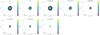 |
Fig. A.1. Emission line maps of GP01. |
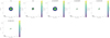 |
Fig. A.2. Emission line maps of GP02. |
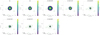 |
Fig. A.3. Emission line maps of GP03. |
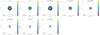 |
Fig. A.4. Emission line maps of GP04. |
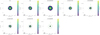 |
Fig. A.5. Emission line maps of GP05. |
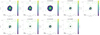 |
Fig. A.6. Emission line maps of GP06. |
 |
Fig. A.7. Emission line maps of GP07. |
 |
Fig. A.8. Emission line maps of GP08. |
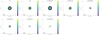 |
Fig. A.9. Emission line maps of GP09. |
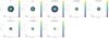 |
Fig. A.10. Emission line maps of GP10. |
 |
Fig. A.11. Emission line maps of GP11. |
 |
Fig. A.12. Emission line maps of GP12. |
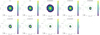 |
Fig. A.13. Emission line maps of GP13. |
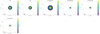 |
Fig. A.14. Emission line maps of GP14. |
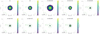 |
Fig. A.15. Emission line maps of GP15. |
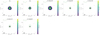 |
Fig. A.16. Emission line maps of GP16. |
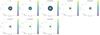 |
Fig. A.17. Emission line maps of GP17. |
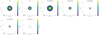 |
Fig. A.18. Emission line maps of GP18. |
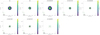 |
Fig. A.19. Emission line maps of GP19. |
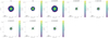 |
Fig. A.20. Emission line maps of GP20. |
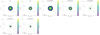 |
Fig. A.21. Emission line maps of GP21. |
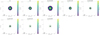 |
Fig. A.22. Emission line maps of GP22. |
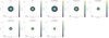 |
Fig. A.23. Emission line maps of GP23. |
 |
Fig. A.24. Emission line maps of GP24. |
Appendix B: Line ratio maps
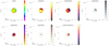 |
Fig. B.1. Line ratio maps for GP01. |
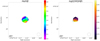 |
Fig. B.2. Line ratio maps for GP02. |
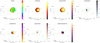 |
Fig. B.3. Line ratio maps for GP03. |
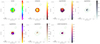 |
Fig. B.4. Line ratio maps for GP04. |
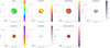 |
Fig. B.5. Line ratio maps for GP05. |
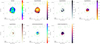 |
Fig. B.6. Line ratio maps for GP06. |
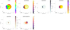 |
Fig. B.7. Line ratio maps for GP07. Spaxels > 20 kpc to the west from the Hα peak are not reliable due to sky contamination. |
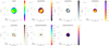 |
Fig. B.8. Line ratio maps for GP08. |
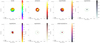 |
Fig. B.9. Line ratio maps for GP09. |
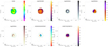 |
Fig. B.10. Line ratio maps for GP10. |
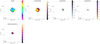 |
Fig. B.11. Line ratio maps for GP11. |
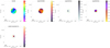 |
Fig. B.12. Line ratio maps for GP12. |
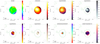 |
Fig. B.13. Line ratio maps for GP13. |
 |
Fig. B.14. Line ratio maps for GP14. |
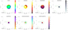 |
Fig. B.15. Line ratio maps for GP15. |
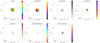 |
Fig. B.16. Line ratio maps for GP16. |
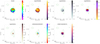 |
Fig. B.17. Line ratio maps for GP17. |
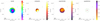 |
Fig. B.18. Line ratio maps for GP18. |
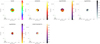 |
Fig. B.19. Line ratio maps for GP19. |
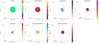 |
Fig. B.20. Line ratio maps for GP20. |
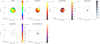 |
Fig. B.21. Line ratio maps for GP21. |
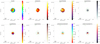 |
Fig. B.22. Line ratio maps for GP22. |
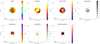 |
Fig. B.23. Line ratio maps for GP23. |
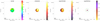 |
Fig. B.24. Line ratio maps for GP24. |
Appendix C: Continuum maps
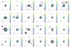 |
Fig. C.1. Continuum maps of all GPs. |
Appendix D: Radial profiles
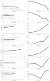 |
Fig. D.1. Radial profiles of remaining emission line ratios. |
Appendix E: Spectra
 |
Fig. E.1. Integrated spectra. |
Appendix F: Emission line data and properties of the ionized gas
Emission line fluxes, extinction and EW of [OIII] line.
continued.
Properties of the ionized gas.
All Tables
All Figures
|
Fig. 1. Redshift histogram of the 24 GPs in our sample. |
| In the text | |
|
Fig. 2. GP06 emission line maps. The black line in the bottom left corresponds to a distance of 10 kpc. The circle in the bottom right is the representation of the seeing. The peak in the Hα emission is represented by the black point in the middle. The green and black contour represents the 3σsky level of the continuum map corresponding to the same galaxy. All maps presented in this work have the previously mentioned features except for the continuum maps, which do not present the continuum contour. Black contours are regions with different signal = k × σsky levels (with k = 10, 100), and all spaxels represented in all maps are above 3σsky. The red contour indicates the FWHM of the map. The same contours are shown in each emission line map and continuum map in this study. |
| In the text | |
|
Fig. 3. Continuum map of GP06. Integration is done between 4154 Å and 7026 in rest frame. |
| In the text | |
|
Fig. 4. Hα/Hβ map of GP06 before reddening correction. |
| In the text | |
|
Fig. 5. [O III]5007/([O II]3727 + [O II]3729) map of GP13. |
| In the text | |
|
Fig. 6. BPT maps corresponding to GP06. |
| In the text | |
|
Fig. 7. Maps corresponding to GP06. |
| In the text | |
|
Fig. 8. Radial profile of Hα/Hβ. The left image shows the profiles of all GPs with available information about the lines in gray. In black it is represented the mean of all galaxies and extends up to a radius where only 30% of the galaxies present values at larger radii. On the right is a zoomed-in image of the mean profile. The same display applies to all line ratios presented in the appendix. |
| In the text | |
|
Fig. 9. BPT diagram. Small dots in the color scale (from yellow to dark purple) correspond to spaxels in each galaxy. Big green dots correspond to the integrated spectra of the galaxy. Next to the green dots we can see the name of each galaxy. The color of the small dots corresponds to the distance to the center of the galaxy. The closer to the center the more yellow they are, and farther away from the center they become darker. The lines that delimitate each region are taken from Kewley et al. (2001) and Kauffmann et al. (2003). |
| In the text | |
|
Fig. 10. Integrated spectrum of GP06. The bottom image is a zoomed-in view of the y-scale of the top image. |
| In the text | |
|
Fig. 11. Stellar mass versus sSFR. Green points are the GPs presented in this work, light green are GPs with HeII emission. The green star represents the median of the GPs, corresponding to a stellar mass of 2.6 × 10⁹ M⊙, an sSFR of 12 Gyr−1, and thus a mass-doubling timescale of 47 Myr. Black points represent a set of local galaxies (z < 0.03) from the Califa survey (Catalán-Torrecilla et al. 2015; Torrecilla15). The black star represents the median of this sample, it corresponds to a stellar mass of 3.2 × 10¹⁰ M⊙, a sSFR of 0.12 Gyr−1 and thus a mass-doubling timescale of 8.3 Gyr, which is on the order of the age of the Universe. We also show the sSFR-mass relation at a variety of redshifts from Tasca et al. (2015; dash-dot line, T15), Karim et al. (2011; dashed line, K11), and Whitaker et al. (2012; dotted line, W12). |
| In the text | |
|
Fig. 12. Electron density, electron temperature, and metallicity representation. Big labeled dots correspond to the six GPs where the direct method can be well applied. The rest of the small dots correspond to all galaxies selected from the NASA-Sloan Atlas with W(λ5007) > 1000 Å and 37 COS Legacy Archive Spectroscopic SurveY galaxies. |
| In the text | |
|
Fig. 13. Oxygen abundance versus stellar mass. GPs are the green points. Black points correspond to ∼200 000 galaxies from Duarte Puertas et al. (2022). |
| In the text | |
|
Fig. 14. Nitrogen over oxygen versus stellar mass. GPs are the green points. Black points correspond to ∼200 000 galaxies from Duarte Puertas et al. (2022). |
| In the text | |
|
Fig. 15. Nitrogen over oxygen versus oxygen abundance. GPs are the green points. Black points correspond to ∼200 000 galaxies from Duarte Puertas et al. (2022). |
| In the text | |
|
Fig. A.1. Emission line maps of GP01. |
| In the text | |
|
Fig. A.2. Emission line maps of GP02. |
| In the text | |
|
Fig. A.3. Emission line maps of GP03. |
| In the text | |
|
Fig. A.4. Emission line maps of GP04. |
| In the text | |
|
Fig. A.5. Emission line maps of GP05. |
| In the text | |
|
Fig. A.6. Emission line maps of GP06. |
| In the text | |
|
Fig. A.7. Emission line maps of GP07. |
| In the text | |
|
Fig. A.8. Emission line maps of GP08. |
| In the text | |
|
Fig. A.9. Emission line maps of GP09. |
| In the text | |
|
Fig. A.10. Emission line maps of GP10. |
| In the text | |
|
Fig. A.11. Emission line maps of GP11. |
| In the text | |
|
Fig. A.12. Emission line maps of GP12. |
| In the text | |
|
Fig. A.13. Emission line maps of GP13. |
| In the text | |
|
Fig. A.14. Emission line maps of GP14. |
| In the text | |
|
Fig. A.15. Emission line maps of GP15. |
| In the text | |
|
Fig. A.16. Emission line maps of GP16. |
| In the text | |
|
Fig. A.17. Emission line maps of GP17. |
| In the text | |
|
Fig. A.18. Emission line maps of GP18. |
| In the text | |
|
Fig. A.19. Emission line maps of GP19. |
| In the text | |
|
Fig. A.20. Emission line maps of GP20. |
| In the text | |
|
Fig. A.21. Emission line maps of GP21. |
| In the text | |
|
Fig. A.22. Emission line maps of GP22. |
| In the text | |
|
Fig. A.23. Emission line maps of GP23. |
| In the text | |
|
Fig. A.24. Emission line maps of GP24. |
| In the text | |
|
Fig. B.1. Line ratio maps for GP01. |
| In the text | |
|
Fig. B.2. Line ratio maps for GP02. |
| In the text | |
|
Fig. B.3. Line ratio maps for GP03. |
| In the text | |
|
Fig. B.4. Line ratio maps for GP04. |
| In the text | |
|
Fig. B.5. Line ratio maps for GP05. |
| In the text | |
|
Fig. B.6. Line ratio maps for GP06. |
| In the text | |
|
Fig. B.7. Line ratio maps for GP07. Spaxels > 20 kpc to the west from the Hα peak are not reliable due to sky contamination. |
| In the text | |
|
Fig. B.8. Line ratio maps for GP08. |
| In the text | |
|
Fig. B.9. Line ratio maps for GP09. |
| In the text | |
|
Fig. B.10. Line ratio maps for GP10. |
| In the text | |
|
Fig. B.11. Line ratio maps for GP11. |
| In the text | |
|
Fig. B.12. Line ratio maps for GP12. |
| In the text | |
|
Fig. B.13. Line ratio maps for GP13. |
| In the text | |
|
Fig. B.14. Line ratio maps for GP14. |
| In the text | |
|
Fig. B.15. Line ratio maps for GP15. |
| In the text | |
|
Fig. B.16. Line ratio maps for GP16. |
| In the text | |
|
Fig. B.17. Line ratio maps for GP17. |
| In the text | |
|
Fig. B.18. Line ratio maps for GP18. |
| In the text | |
|
Fig. B.19. Line ratio maps for GP19. |
| In the text | |
|
Fig. B.20. Line ratio maps for GP20. |
| In the text | |
|
Fig. B.21. Line ratio maps for GP21. |
| In the text | |
|
Fig. B.22. Line ratio maps for GP22. |
| In the text | |
|
Fig. B.23. Line ratio maps for GP23. |
| In the text | |
|
Fig. B.24. Line ratio maps for GP24. |
| In the text | |
|
Fig. C.1. Continuum maps of all GPs. |
| In the text | |
|
Fig. D.1. Radial profiles of remaining emission line ratios. |
| In the text | |
|
Fig. E.1. Integrated spectra. |
| In the text | |
Current usage metrics show cumulative count of Article Views (full-text article views including HTML views, PDF and ePub downloads, according to the available data) and Abstracts Views on Vision4Press platform.
Data correspond to usage on the plateform after 2015. The current usage metrics is available 48-96 hours after online publication and is updated daily on week days.
Initial download of the metrics may take a while.