| Issue |
A&A
Volume 676, August 2023
|
|
|---|---|---|
| Article Number | L1 | |
| Number of page(s) | 10 | |
| Section | Letters to the Editor | |
| DOI | https://doi.org/10.1051/0004-6361/202347174 | |
| Published online | 25 July 2023 | |
Letter to the Editor
Discovery of H2CCCH+ in TMC-1⋆
1
I. Physikalisches Institut, Universität zu Köln, Zülpicher Str. 77, 50937 Köln, Germany
e-mail: This email address is being protected from spambots. You need JavaScript enabled to view it.
2
Dept. de Astrofísica Molecular, Instituto de Física Fundamental (IFF-CSIC), Serrano 121, 28006 Madrid, Spain
3
Centro de Desarrollos Tecnológicos, Observatorio de Yebes (IGN), 19141 Yebes, Guadalajara, Spain
4
Observatorio Astronómico Nacional (OAN, IGN), Madrid, Spain
5
Institut des Sciences Moléculaires (ISM), CNRS, Univ. Bordeaux, 351 cours de la Libération, 33400 Talence, France
6
Laboratoire d’Astrophysique de Bordeaux, Univ. Bordeaux, CNRS, B18N, allée Geoffroy Saint-Hilaire, 33615 Pessac, France
7
, Serrano 123, 28006 Madrid, Spain
Received:
13
June
2023
Accepted:
3
July
2023
Abstract
Based on a novel laboratory method, 14 millimeter-wave lines of the molecular ion H2CCCH+ have been measured in high resolution, and the spectroscopic constants of this asymmetric rotor determined with high accuracy. Using the Yebes 40 m and IRAM 30 m radio telescopes, we detected four lines of H2CCCH+ toward the cold dense core TMC-1. With a dipole moment of about 0.55 D obtained from high-level ab initio calculations, we derive a column density of 5.4±1×1011 cm−2 and 1.6±0.5×1011 cm−2 for the ortho and para species, respectively, and an abundance ratio N(H2CCC)/N(H2CCCH+) = 2.8±0.7. The chemistry of H2CCCH+ is modeled using the most recent chemical network for the reactions involving the formation of H2CCCH+. We find a reasonable agreement between model predictions and observations, and new insights into the chemistry of C3-bearing species in TMC-1 were obtained.
Key words: astrochemistry / ISM: molecules / ISM: individual objects: TMC-1 / methods: laboratory: molecular / molecular data / line: identification
Based on observations carried out with the Yebes 40 m telescope (projects 19A003, 20A014, 20D15, and 21A011) and the Institut de Radioastronomie Millimétrique (IRAM) 30 m telescope. The 40 m radiotelescope at Yebes Observatory is operated by the Spanish Geographic Institute (IGN, Ministerio de Transportes, Movilidad y Agenda Urbana). IRAM is supported by INSU/CNRS (France), MPG (Germany), and IGN (Spain).
© The Authors 2023
 Open Access article, published by EDP Sciences, under the terms of the Creative Commons Attribution License (https://creativecommons.org/licenses/by/4.0), which permits unrestricted use, distribution, and reproduction in any medium, provided the original work is properly cited.
This article is published in open access under the Subscribe to Open model. This email address is being protected from spambots. You need JavaScript enabled to view it. to support open access publication.
1. Introduction
Molecular ions are important intermediates in the chemistry of the interstellar medium (ISM). These charged species can rapidly react with neutral partners or recombine with electrons to form other ionic and neutral molecules under astrophysical conditions (Larsson et al. 2012; Agúndez & Wakelam 2013). Despite their fundamental role in astrochemistry, many ions remain elusive mainly due to their highly reactive character and lack of accurate laboratory data to support astronomical detections (McGuire et al. 2020). Consequently, many ions in astrochemical models and theories await confirmation through spectroscopic detection in the ISM.
One example is the formation of the hydrocarbons C3H2 and C3H, whose cyclic isomers (c-C3H2 and c-C3H) and linear isomers (l-C3H2 and l-C3H, i.e., H2CCC and HCCC, respectively) were both detected in the ISM (Thaddeus et al. 1985a,b; Yamamoto et al. 1987; Cernicharo et al. 1991), and even deuterated versions were observed (Bell et al. 1986; Spezzano et al. 2013, 2016; Agúndez et al. 2019). The synthesis of the cyclic and linear forms of C3H2 and C3H is thought to occur via the dissociative recombination of the respective isomers of C3H , c-C3H
 and H2CCCH+, with electrons (Maluendes et al. 1993). In turn, the two isomers of C3H
 are thought to be produced through the radiative association of C3H+ and H2 (Savić & Gerlich 2005). The proof of this chemical pathway for the cyclic variants is difficult because c-C3H
 is a symmetric molecule and can only be detected based on its rovibrational fingerprints in the infrared (Zhao et al. 2014), which might be feasible with the James Webb Space Telescope (JWST) in the near future. While the singly deuterated version c-C3H2D+ could be probed by radio astronomy, it has a predicted low dipole moment and low column densities (Gupta et al. 2023). This leaves only H2CCCH+ as a good candidate for radio astronomical searches.
In this Letter, based on a novel experimental method, we report the first laboratory millimeter-wave data of H2CCCH+ and its radio-astronomical detection toward the cold dark core TMC-1. We derive its column density toward TMC-1 and discuss these results in the context of state-of-the-art chemical models.
2. Laboratory work
H2CCCH+ is a closed-shell, planar, and near-prolate asymmetric top molecular ion (see sketch in Fig. 1). H2CCCH+ ions were generated in the Cologne laboratory in a storage ion source via electron impact ionization (Ee ≈ 30 eV) of the precursor gas allene (C3H4). By applying a novel trap-based technique called leak-out spectroscopy (LOS, Schmid et al. 2022) in the cryogenic ion trap machine COLTRAP (Asvany et al. 2010, 2014), the vibrational bands ν1 and ν3 + ν5 were measured in the range 3180–3240 cm−1 in high resolution. The vibrational measurements, whose details will be described in a forthcoming publication, enabled the ground state spectroscopic parameters of H2CCCH+ to be determined. Subsequently, pure rotational lines were detected using a vibrational-rotational double resonance (DR) method. Such methods have been reviewed by Asvany & Schlemmer (2021), and the particular scheme involving LOS has only recently been demonstrated by Asvany et al. (2023). An example measurement for H2CCCH+ is shown in Fig. 1.
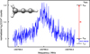 |
Fig. 1. Pure rotational transition ( |

Double resonance spectra were recorded in multiple individual measurements in which the millimeter-wave frequency (blue arrow in Fig. 1) was stepped in an up-and-down manner several times. Selected rovibrational lines from the ν1 or the ν3 + ν5 combination band were used for the IR excitation (red arrow in Fig. 1). The frequency steps of the millimeter-wave radiation were kept constant in individual experiments, and varied between 3 and 50 kHz; the larger steps were typically used to search for new lines. The spectroscopic data were normalized employing a frequency switching procedure, in which the H2CCCH+ counts monitored while scanning the spectral range of interest are divided by the counts at an off-resonant millimeter-wave reference frequency. Therefore, the baseline in Fig. 1 is close to unity. The on-resonance signal enhancement is on the order of 15%. Transition frequencies were determined by adjusting the parameters of an appropriate line shape function (typically a Gaussian) to the experimental spectrum in a least-squares procedure. In total, 14 rotational lines were detected in the laboratory and are summarized in Table 1. The frequencies and their uncertainties in the table result from the weighted average of up to 11 independent line-center determinations for each transition.
Ground state rotational transition frequencies of H2CCCH+, determined by laboratory and astronomical detections.
The fit of the assigned lines (lab + astro) was carried out using Watson’s S-reduced Hamiltonian in the Ir representation, as implemented in Western’s PGOPHER program (Western 2017). The resulting spectroscopic parameters are given in Table 2. As H2CCCH+ is a near-prolate asymmetric top (κ = −0.9976) with an a-type spectrum, the A0 rotational constant is not well constrained from experiment. Overall, the experimental rotational and centrifugal distortion constants compare favorably with those calculated by Huang et al. (2011) and very well with the best estimate values obtained in this study (given in the last three columns of Table 2). The obtained obs-calc values for the rotational lines are given in Table 1. In total, the weighted rms of the fit is on the order of 1.4, indicating somewhat optimistic uncertainties of our measurements.
3. Quantum chemical calculations
The H2CCCH+ molecular ion has been the subject of several quantum-chemical investigations in the past (e.g., Botschwina et al. 1993, 2011; Huang et al. 2011; Marimuthu et al. 2020, and references therein). In the present study, complementary high-level calculations were performed at the CCSD(T) level of theory (Raghavachari et al. 1989) together with correlation consistent (augmented) polarized weighted core-valence basis sets (Kendall et al. 1992; Peterson & Dunning 2002) and atomic natural orbital basis sets (Almlöf & Taylor 1987). All calculations were performed using the CFOUR program suite (Matthews et al. 2020; Harding et al. 2008). Equilibrium rotational constants were calculated at the all-electron (ae-)CCSD(T)/cc-pwCVQZ level of theory that is known to yield molecular equilibrium structural parameters of very high quality for molecules comprising first- and second-row elements (e.g., Coriani et al. 2005).
Zero-point vibrational contributions  ) to the equilibrium rotational constants and centrifugal distortion parameters were calculated at the frozen core (fc-)CCSD(T)/ANO1 level. Best estimate (BE, Tables 2 and A.1) rotational and centrifugal distortion constants were finally obtained through empirical scaling of the calculated rotational parameters using factors (i.e., the ratios Xexp/Xcalc of a given parameter) derived from isoelectronic propadienylidene, H2CCC, the pure rotational spectrum of which is known well from a previous study (Vrtilek et al. 1990). The technique of empirical scaling using structurally closely related (isoelectronic) species known from experiment may provide rotational parameters at a predictive power greatly exceeding that of high-level calculations alone (see, e.g., Thorwirth et al. 2005, 2020; Martinez et al. 2013), and has been used recently to identify species not studied in the laboratory using radio astronomy (see, e.g., Cernicharo et al. 2020b).
The dipole moment of H2CCCH+ is not very large. At the ae-CCSD(T)/aug-cc-pwCVQZ level of theory the (center-of-mass frame) equilibrium value μe amounts to 0.53 D, in good agreement with earlier estimates. Zero-point vibrational effects (fc-CCSD(T)/ANO1) have an almost negligible influence resulting in μ0 = 0.55 D.
4. Observations
New receivers, built within the Nanocosmos1 project and installed at the Yebes 40 m radio telescope, were used for the observations of TMC-1 (αJ2000 = 4h41m41.9s and δJ2000 = +25° 41′27.0″). The observations of TMC-1 belong to the ongoing QUIJOTE2 line survey (Cernicharo et al. 2021a, 2023). A detailed description of the telescope, receivers, and backends is given by Tercero et al. (2021). Briefly, the receiver consists of two cold high electron mobility transistor amplifiers covering the 31.0–50.3 GHz band with horizontal and vertical polarizations. The backends are 2 × 8 × 2.5 GHz fast Fourier transform spectrometers with a spectral resolution of 38.15 kHz providing the coverage of the whole Q-band in both polarizations.
The observations, carried out during different observing runs, were performed using the frequency-switching mode with a frequency throw of 10 MHz in the very first observing runs, during November 2019 and February 2020, 8 MHz during the observations of January–November 2021, and alternating these frequency throws in the last observing runs between October 2021 and February 2023. The total on-source telescope time is 850 h in each polarization (385 and 465 h for the 8 MHz and 10 MHz frequency throws, respectively). The sensitivity of the QUIJOTE line survey varies between 0.17 and 0.25 mK in the 31–50.3 GHz domain. The intensity scale used in this work, antenna temperature ( ), was calibrated using two absorbers at different temperatures and the atmospheric transmission model ATM (Cernicharo 1985; Pardo et al. 2001). The calibration uncertainties adopted were 10%. The beam efficiency of the Yebes 40 m telescope in the Q-band is given as a function of frequency by Beff = 0.797 exp[−(ν(GHz)/71.1)2]. The forward telescope efficiency is 0.97. The telescope beam size varies from 56.7″ at 31 GHz to 35.6″ at 49.5 GHz.
The data of TMC-1 taken with the IRAM 30 m telescope consist of a 3 mm line survey obtained with the old ABCD receivers connected to an autocorrelator that provided a spectral resolution of 40 kHz (Marcelino et al. 2007; Cernicharo et al. 2012). Some additional high-sensitivity frequency windows observed in 2021 used the new 3 mm EMIR dual polarization receiver connected to four fast Fourier transform spectrometers providing a spectral resolution of 49 kHz (Agúndez et al. 2022; Cabezas et al. 2022a). All the observations were performed using the frequency switching method. The final 3 mm line survey has a sensitivity of 2–10 mK. However, at some selected frequencies the sensitivity is as low as 0.6 mK.
5. Detection of H2CCCH+ in TMC-1
We searched for one para (202-101) and two ortho (212-111, 211-110) lines of H2CCCH+ within the QUIJOTE line survey. The three lines were clearly detected and are shown in Fig. 2. In the data at 3 mm we covered the frequencies of three para and four ortho lines, with upper levels J = 4, 5, 6 and energies below 30 K. Only one line, the J = 514 − 413, falls in one of the high-sensitivity windows (σ = 0.6 mK) of our line survey, and it was also clearly detected (see Fig. 2). Two other lines are within frequency ranges with σ below 2 mK, and were marginally detected. The derived line parameters for all searched transitions of H2CCCH+ are given in Table B.1. We checked that the detected lines cannot be assigned to lines of other species or isotopologs by exploring the spectral catalogs MADEX (Cernicharo 2012), CDMS (Müller et al. 2005), and JPL (Pickett et al. 1998).
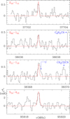 |
Fig. 2. Lines of H2CCCH+ observed in the 31–115 GHz domain toward TMC-1. The abscissa corresponds to the rest frequency in MHz. The ordinate is the antenna temperature corrected for atmospheric and telescope losses in mK. The spectral resolution is 38 kHz below 50 GHz and 48 kHz above. The line parameters are given in Table B.1. The red lines show the computed synthetic spectra (see text). |
To estimate the column density of H2CCCH+, we considered the ortho and para levels as belonging to two different species. For the dipole moment we used the value of 0.55 D calculated in this work. No collisional rates are available for this molecule. However, Khalifa et al. (2019) computed the collisional rates between He and H2CCC. This cumulenic species is isoelectronic with our molecule and has a very similar structure. We therefore adopted these rates, correcting for the abundance of He with respect to H2, to estimate the excitation temperatures of the observed transitions of H2CCCH+. Assuming a volume density of (1–3)×104 cm−3 (Fossé et al. 2001; Lique et al. 2006; Pratap et al. 1997), we derive excitation temperatures close to 10 K for the J = 2-1 lines, and ∼8–10 K for the lines in the 3 mm domain, the largest value corresponding to n(H2) = 3×104 cm−3. These excitation temperatures are considerably larger than those obtained for H2CCC, which are between 4 and 5 K, due to the larger dipole moment of this species (4.1 vs. 0.55 D). From the adopted rotational temperatures of 9 K, and assuming a source of uniform brightness temperature with a radius of 40″ (Fossé et al. 2001), we derive a column density for ortho-H2CCCH+ of (5.4±1)×1011 cm−2. For the para species the estimated column density is (1.6±0.5)×1011 cm−2, a value that is consistent with the expected ortho to para ratio of 3/1. The computed synthetic spectra show excellent agreement with the observed line intensities (see Fig. 2). Hence, the total column density of H2CCCH+ in TMC-1 is (7.0±1.5)×1011 cm−2.
It is interesting to compare the abundance of H2CCCH+ to that of H2CCC. For the latter species we detected, with an excellent signal-to-noise ratio, all its ortho and para lines in the frequency range of our line surveys. The derived line parameters are summarized in Table B.2 and the lines are shown in Fig. B.1. The decline of the line intensity between the Ju = 2 and Ju = 5 lines is obvious in Fig. B.1, which indicates that the lines are not thermalized to the kinetic temperature of the cloud for this species. Using the collisional rates of Khalifa et al. (2019), and adopting the same assumptions on the source size as for H2CCCH+, we derive a column density for the ortho and para species of (1.5±0.1)×1012 and (0.45±0.05)×1012 cm−2, respectively. The best fit is obtained for a density of n(H2) = 8×103 cm−3. The total column density of H2CCC is (1.95±0.15)×1012 cm−2 and the ortho-to-para ratio for this species is 3.3±0.6. The H2CCC/H2CCCH+ abundance ratio is 2.8±0.7 which is on the order of that found for C3O/HC3O+ (Cernicharo et al. 2020b), but much lower than the abundance ratio found in TMC-1 for other neutral species and their protonated forms (Marcelino et al. 2020; Cernicharo et al. 2021b,c; Cabezas et al. 2022b; Agúndez et al. 2022).
6. Discussion
To describe the chemistry of H2CCCH+, we used the Nautilus code (Ruaud et al. 2016), a three-phase (gas, dust grain ice surface, and dust grain ice mantle) time-dependent chemical model with a chemical network for C3H species very similar to that presented in Loison et al. (2017). To describe the physical conditions in TMC-1, we used a homogeneous cloud with a density equal to 2.5×104 cm−3, a temperature equal to 10 K for both the gas and the dust, a visual extinction of 30 mag, and a cosmic-ray ionization rate of 1.3×10⁻¹⁷ s−1. All elements are assumed to be initially in atomic form, except for hydrogen, which is entirely molecular (Hincelin et al. 2011). The calculated abundances relative to H2 for H2CCC and H2CCCH+, and also for C3 and C3H+, which are strongly linked to H2CCCH+, are shown in Fig. 3.
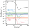 |
Fig. 3. Abundances of C3, C3H+, H2CCC, and H2CCCH+ as a function of time predicted by our model (continuous lines). The horizontal colored areas represent the observations in TMC-1 assuming an uncertainty of 3 on the measurements (Cernicharo et al. 2022 for C3H+ and this work for H2CCCH+). Dashed lines: Same, but with a threefold decrease in the H2 + C3H+ and a fivefold increase in the H2CCCH+ + e− rate coefficients. The vertical gray area represents the values given by the most probable chemical age for TMC-1, due to the better agreement between calculations and observations for 67 key species. |
As can be seen in Fig. 3, the H2CCC and H2CCCH+ abundances observed are relatively well reproduced by the model for a relatively early molecular cloud age of around 2×10⁵ years, however, with a lower H2CCC/H2CCCH+ ratio than the one observed. Looking in more detail at the chemistry of H2CCCH+ and H2CCC (see Fig. 3 of Loison et al. 2017), it appears that H2CCC is a product of H2CCCH+ (and also of c-C3H ), but that the flow of protonation of H2CCC toward H2CCCH+ is a very minor pathway for the formation of H2CCCH+, which is almost essentially produced by the reaction C3H+ + H2. This inverted link between H2CCC and H2CCCH+ explains the unusually high MH+/M ratio compared to those cases in which the protonated form comes from the protonation of the neutral form (Agúndez et al. 2022).
Considering the link between C3H+, H2CCCH+, and C3, it is interesting to see if the observations of H2CCCH+ (this work) combined to the observation of C3H+ (Cernicharo et al. 2022) allow us to estimate the abundance of C3, which in our dense cloud model is the second carbon reservoir, accounting for up to 15% of carbon. If C3 does not react with atomic oxygen, as calculated by Woon & Herbst (1996), the protonation reactions of C3 producing C3H+ are by far the main reactions of destruction of C3 and of production of C3H+. As these protonation reactions control the destruction of C3, the uncertainties on the rates affect the abundance of C3, but do not change the flux of these reactions. The underestimation of C3H+ in the model is therefore not related to these protonation rates, but to the rate of the reaction C3H+ + H2, which controls the destruction of C3H+ (Maluendes et al. 1993; Savić & Gerlich 2005). A decrease in the rate of the reaction C3H+ + H2 at 10 K by a factor of 3 allows us to reproduce the abundance of C3H+ observed by Cernicharo et al. (2022), as shown in Fig. 3. This change in the rate coefficient does not affect the flux of the C3H+ + H2 reaction, and therefore does not affect the abundance of H2CCCH+, as long as the branching ratios to H2CCCH+ and c-C3H are not varied. Since H2CCCH+ is mainly destroyed by the reaction with electrons, its abundance is controlled by the rate of this reaction, which is known only over the temperature range 172–489 K (McLain et al. 2005) with a temperature dependency inconsistent with theory. An increase in this rate at 10 K by a factor of 5, which is not impossible given the uncertainties, allows us to reproduce the observation for H2CCCH+ with a ratio between H2CCC/H2CCCH+ that is very close to the observed value. Considering the uncertainties of the different chemical reactions linking C3 to C3H+ and H2CCCH+, the observations of C3H+ (Cernicharo et al. 2022) and H2CCCH+ (this work) validate the chemical scheme controlling the formation of cyclic and linear C3H and C3H2 and the high gas-phase abundance of C3 in TMC-1, around 10−6 relative to H2.
It would also be very interesting to know the abundance of the more stable cyclic isomer c-C3H , which in the chemical model is predicted to be slightly more abundant (by a factor of three) than H2CCCH+. This species has no dipole moment, but its deuterated version, c-C3H2D+, has a low dipole moment of 0.225 D (Huang & Lee 2011) and its rotational spectrum has been recently measured in the 90–230 GHz frequency range in Cologne (Gupta et al. 2023). We searched for c-C3H2D+ in the QUIJOTE line survey but at the current level of sensitivity, this species is not detected and we derive an upper limit to its column density of 4×1012 cm−3. Assuming that the c-C3H
 /c-C3H2D+ ratio is 10, as found for the analog case of CH3CCH with three equivalent H nuclei (Cabezas et al. 2021), the column density of c-C3H
 is < 4×1013 cm−2, which is not very meaningful.
ERC grant ERC-2013-Syg-610256-NANOCOSMOS.
Q-band Ultrasensitive Inspection Journey to the Obscure TMC-1 Environment
Acknowledgments
The work has been supported by an ERC advanced grant (MissIons: 101020583), the Deutsche Forschungsgemeinschaft (DFG) via SFB 956 (project ID 184018867), sub-project B2, and the Gerätezentrum “Cologne Center for Terahertz Spectroscopy” (DFG SCHL 341/15-1). W.G.D.P.S. thanks the Alexander von Humboldt foundation for funding through a postdoctoral fellowship. We also acknowledge the support from the MICINN projects PID2020-113084GB-I00 and PID2019-106110GB-I00, the CSIC project ILINK+ LINKA20353, the ERC grant ERC-2013-Syg610256-NANOCOSMOS, and the Regional Computing Center of the Universität zu Köln (RRZK) for providing computing time on the DFG-funded high performance computing system CHEOPS.
References
- Agúndez, M., & Wakelam, V. 2013, Chem. Rev., 113, 8710 [Google Scholar]
- Agúndez, M., Marcelino, N., Cernicharo, J., Roueff, E., & Tafalla, M. 2019, A&A, 625, A147 [Google Scholar]
- Agúndez, M., Cabezas, C., Marcelino, N., et al. 2022, A&A, 659, L9 [NASA ADS] [CrossRef] [EDP Sciences] [Google Scholar]
- Almlöf, J., & Taylor, P. R. 1987, J. Chem. Phys., 86, 4070 [CrossRef] [Google Scholar]
- Asvany, O., & Schlemmer, S. 2021, Phys. Chem. Chem. Phys., 23, 26602 [NASA ADS] [CrossRef] [Google Scholar]
- Asvany, O., Bielau, F., Moratschke, D., Krause, J., & Schlemmer, S. 2010, Rev. Sci. Instruct., 81, 076102 [NASA ADS] [CrossRef] [Google Scholar]
- Asvany, O., Brünken, S., Kluge, L., & Schlemmer, S. 2014, Appl. Phys. B, 114, 203 [NASA ADS] [CrossRef] [Google Scholar]
- Asvany, O., Thorwirth, S., Schmid, P., Salomon, T., & Schlemmer, S. 2023, Phys. Chem. Chem. Phys., https://dx.doi.org/10.1039/D3CP01976D [Google Scholar]
- Bell, M. B., Feldman, P. A., Matthews, H. E., & Avery, L. W. 1986, ApJ, 311, L89 [Google Scholar]
- Botschwina, P., Horn, M., Flügge, J., & Seeger, S. 1993, J. Chem. Soc. Faraday Trans., 89, 2219 [Google Scholar]
- Botschwina, P., Oswald, R., & Rauhut, G. 2011, PCCP, 13, 7921 [NASA ADS] [CrossRef] [Google Scholar]
- Cabezas, C., Agúndez, M., Marcelino, N., et al. 2022a, A&A, 657, L4 [NASA ADS] [CrossRef] [EDP Sciences] [Google Scholar]
- Cabezas, C., Agúndez, M., Marcelino, N., et al. 2022b, A&A, 659, L8 [NASA ADS] [CrossRef] [EDP Sciences] [Google Scholar]
- Cabezas, C., Endo, Y., Roueff, E., et al. 2021, A&A, 646, L1 [NASA ADS] [CrossRef] [EDP Sciences] [Google Scholar]
- Cernicharo, J. 1985, IRAM Internal Report [Google Scholar]
- Cernicharo, J. 2012, in ECLA2011; Proc. of the European Conference on Laboratory Astrophysics, eds. C. Stehl, C. Joblin, & L. d’Hendecourt (Cambridge: Cambridge Univ. Press), EAS Publ. Ser., 251 [Google Scholar]
- Cernicharo, J., Gottlieb, C. A., Guelin, M., et al. 1991, ApJ, 368, L39 [NASA ADS] [CrossRef] [Google Scholar]
- Cernicharo, J., Marcelino, N., Roueff, E., et al. 2012, ApJ, 759, L43 [NASA ADS] [CrossRef] [Google Scholar]
- Cernicharo, J., Marcelino, N., Agúndez, M., et al. 2020a, A&A, 642, L8 [NASA ADS] [CrossRef] [EDP Sciences] [Google Scholar]
- Cernicharo, J., Marcelino, N., Agúndez, M., et al. 2020b, A&A, 642, L17 [NASA ADS] [CrossRef] [EDP Sciences] [Google Scholar]
- Cernicharo, J., Agúndez, M., Kaiser, R., et al. 2021a, A&A, 652, L9 [NASA ADS] [CrossRef] [EDP Sciences] [Google Scholar]
- Cernicharo, J., Cabezas, C., Endo, Y., et al. 2021b, A&A, 646, L3 [EDP Sciences] [Google Scholar]
- Cernicharo, J., Cabezas, C., Bailleux, S., et al. 2021c, A&A, 646, L7 [NASA ADS] [CrossRef] [EDP Sciences] [Google Scholar]
- Cernicharo, J., Agúndez, M., Cabezas, C., et al. 2022, A&A, 657, L16 [NASA ADS] [CrossRef] [EDP Sciences] [Google Scholar]
- Cernicharo, J., Pardo, J., Cabezas, C., et al. 2023, A&A, 670, L19 [NASA ADS] [CrossRef] [EDP Sciences] [Google Scholar]
- Coriani, S., Marcheson, D., Gauss, J., et al. 2005, J. Chem. Phys., 123, 184107 [NASA ADS] [CrossRef] [Google Scholar]
- Fossé, D., Cernicharo, J., Gerin, M., & Cox, P. 2001, ApJ, 552, 168 [Google Scholar]
- Gupta, D., Dias de Paiva Silva, W. G., Doménech, J. L., et al. 2023, Faraday Discuss., https://doi.org/10.1039/D3FD00068K [Google Scholar]
- Harding, M. E., Metzroth, T., Gauss, J., & Auer, A. A. 2008, J. Chem. Theory Comput., 4, 64 [CrossRef] [Google Scholar]
- Hincelin, U., Wakelam, V., Hersant, F., et al. 2011, A&A, 530, A61 [NASA ADS] [CrossRef] [EDP Sciences] [Google Scholar]
- Huang, X., & Lee, T. J. 2011, ApJ, 736, 33 [NASA ADS] [CrossRef] [Google Scholar]
- Huang, X., Taylor, P. R., & Lee, T. J. 2011, J. Phys. Chem. A, 115, 5005 [NASA ADS] [CrossRef] [Google Scholar]
- Kendall, R. A., Dunning, T. H., & Harrison, R. J. 1992, J. Chem. Phys, 96, 6796 [NASA ADS] [CrossRef] [Google Scholar]
- Khalifa, M. B., Sahnoun, E., Wiesenfeld, L., et al. 2019, PCCP, 21, 1443 [NASA ADS] [CrossRef] [Google Scholar]
- Larsson, M., Geppert, W. D., & Nyman, G. 2012, Rep. Prog. Phys., 75, 066901 [NASA ADS] [CrossRef] [Google Scholar]
- Lique, F., Cernicharo, J., & Cox, P. 2006, ApJ, 653, 1342 [NASA ADS] [CrossRef] [Google Scholar]
- Loison, J.-C., Agúndez, M., Wakelam, V., et al. 2017, MNRAS, 470, 4075 [Google Scholar]
- Maluendes, S. A., McLean, A. D., & Herbst, E. 1993, ApJ, 417, 181 [NASA ADS] [CrossRef] [Google Scholar]
- Marcelino, N., Cernicharo, J., Agúndez, M., et al. 2007, ApJ, 665, L127 [Google Scholar]
- Marcelino, N., Agúndez, M., Tercero, B., et al. 2020, A&A, 643, L6 [NASA ADS] [CrossRef] [EDP Sciences] [Google Scholar]
- Marimuthu, A. N., Sundelin, D., Thorwirth, S., et al. 2020, J. Mol. Spectrosc., 374, 111377 [Google Scholar]
- Martinez, O., Jr, Lattanzi, V., Thorwirth, S., & McCarthy, M. C. 2013, J. Chem. Phys., 138, 094316 [NASA ADS] [CrossRef] [Google Scholar]
- Matthews, D. A., Cheng, L., Harding, M. E., et al. 2020, J. Chem. Phys., 152, 214108 [NASA ADS] [CrossRef] [Google Scholar]
- McGuire, B. A., Asvany, O., Brünken, S., & Schlemmer, S. 2020, Nat. Rev. Phys., 2, 402 [NASA ADS] [CrossRef] [Google Scholar]
- McLain, J. L., Poterya, V., Molek, C. D., et al. 2005, J. Phys. Chem. A, 109, 5119 [NASA ADS] [CrossRef] [Google Scholar]
- Müller, H., Schlöder, F., Stutzki, J., & Winnewisser, G. 2005, J. Mol. Struc., 742, 215 [CrossRef] [Google Scholar]
- Pardo, J., Cernicharo, J., & Serabyn, E. 2001, IEEE Trans. Antenn. Propag., 49, 12 [Google Scholar]
- Peterson, K. A., & Dunning, T. H. 2002, J. Chem. Phys., 117, 10548 [NASA ADS] [CrossRef] [Google Scholar]
- Pickett, H., Poynter, R., Cohen, E., et al. 1998, J. Quant. Spectrosc. Radiat. Transf., 60, 883 [NASA ADS] [CrossRef] [Google Scholar]
- Pratap, P., Dickens, J., Snell, R., et al. 1997, ApJ, 486, 862 [NASA ADS] [CrossRef] [Google Scholar]
- Raghavachari, K., Trucks, G. W., Pople, J. A., & Head-Gordon, M. 1989, Chem. Phys. Lett., 157, 479 [Google Scholar]
- Ruaud, M., Wakelam, V., & Hersant, F. 2016, MNRAS, 459, 3756 [Google Scholar]
- Savić, I., & Gerlich, D. 2005, PCCP, 7, 1026 [Google Scholar]
- Schmid, P. C., Asvany, O., Salomon, T., Thorwirth, S., & Schlemmer, S. 2022, J. Phys. Chem. A, 126, 8111 [NASA ADS] [CrossRef] [Google Scholar]
- Spezzano, S., Brünken, S., Schilke, P., et al. 2013, ApJ, 769, L19 [Google Scholar]
- Spezzano, S., Gupta, H., Brünken, S., et al. 2016, A&A, 586, A110 [NASA ADS] [CrossRef] [EDP Sciences] [Google Scholar]
- Tercero, F., López-Pérez, J. A., Gallego, J. D., et al. 2021, A&A, A37, 552 [Google Scholar]
- Thaddeus, P., Gottlieb, C. A., Hjalmarson, A., et al. 1985a, ApJ, 294, L49 [NASA ADS] [CrossRef] [Google Scholar]
- Thaddeus, P., Vrtilek, J. M., & Gottlieb, C. A. 1985b, ApJ, 299, L63 [NASA ADS] [CrossRef] [Google Scholar]
- Thorwirth, S., McCarthy, M. C., Dudek, J. B., & Thaddeus, P. 2005, J. Chem. Phys., 122, 184308 [NASA ADS] [CrossRef] [Google Scholar]
- Thorwirth, S., Harding, M. E., Asvany, O., et al. 2020, Mol. Phys., 118, e1776409 [Google Scholar]
- Vrtilek, J. M., Gottlieb, C. A., Gottlieb, E. W., Killian, T. C., & Thaddeus, P. 1990, ApJ, 364, L53 [NASA ADS] [CrossRef] [Google Scholar]
- Western, C. M. 2017, J. Quant. Spectrosc. Radiat. Transf., 186, 221 [NASA ADS] [CrossRef] [Google Scholar]
- Woon, D. E., & Herbst, E. 1996, ApJ, 465, 795 [NASA ADS] [CrossRef] [Google Scholar]
- Yamamoto, S., Saito, S., Ohishi, M., et al. 1987, ApJ, 322, L55 [Google Scholar]
- Zhao, D., Doney, K. D., & Linnartz, H. 2014, ApJ, 791, L28 [NASA ADS] [CrossRef] [Google Scholar]
Appendix A: Structural calculations, internal coordinates
Bond lengths are given in Å; angles are given in degrees.
A.1. H2CCCH+
H2C3H+, CCSD(T)/cc-pwCVQZ
H
C 1 r1
X 2 rd 1 a90
C 2 r2 3 a90 1 d180
X 4 rd 2 a90 3 d0
C 4 r3 5 a90 2 d180
H 6 r4 4 a1 5 d0
H 6 r4 4 a1 5 d180
r1   =        1.073118130747218
rd   =        1.000000818629780
a90  =       90.000000000000000
r2   =        1.228490857165352
d180 =      180.000000000000000
d0   =        0.000000000000000
r3   =        1.346565030012042
r4   =        1.086025065701484
a1   =      120.382476682815607
H2C3H+, CCSD(T)/ANO1
H
C 1 r1
X 2 rd 1 a90
C 2 r2 3 a90 1 d180
X 4 rd 2 a90 3 d0
C 4 r3 5 a90 2 d180
H 6 r4 4 a1 5 d0
H 6 r4 4 a1 5 d180
r1   =        1.074705266639338
rd   =        1.000000204657382
a90  =       90.000000000000000
r2   =        1.234261558515133
d180 =      180.000000000000000
d0   =        0.000000000000000
r3   =        1.351397370372584
r4   =        1.088292080166718
a1   =      120.373581553220575
A.2. H2CCC
H2CCC, CCSD(T)/cc-pwCVQZ
C
C 1 r1
X 2 rd 1 a90
C 2 r2 3 a90 1 d180
H 4 r3 2 a1 3 d0
H 4 r3 2 a1 5 d180
r1   =        1.287645153115967
rd   =        1.000000000000000
a90  =       90.000000000000000
r2   =        1.327897213723068
d180 =      180.000000000000000
r3   =        1.083584615827809
a1   =      121.271597504509145
d0   =        0.000000000000000
H2CCC, CCSD(T)/ANO1
C
C 1 r1
X 2 rd 1 a90
C 2 r2 3 a90 1 d180
H 4 r3 2 a1 3 d0
H 4 r3 2 a1 5 d180
r1   =        1.294632885150227
rd   =        1.000000204657382
a90  =       90.000000000000000
r2   =        1.333030062830918
d180 =      180.000000000000000
r3   =        1.085894615830395
a1   =      121.302559724582778
d0   =        0.000000000000000
Calculated and experimental spectroscopic parameters of H2CCC and H2CCCH+ (in MHz). Equilibrium rotational constants calculated at the ae-CCSD(T)/cc-pwCVQZ level of theory; zero-point vibrational corrections ΔA0, ΔB0, ΔC0; and centrifugal distortion constants calculated at the fc-CCSD(T)/ANO1 level. Best theoretical estimates for the rotational and centrifugal distortion constants X of H2CCCH+ are estimated as  (i.e., using isoelectronic H2CCC as a calibrator).
Appendix B: Line parameters of H2CCCH+ and H2CCC
The line parameters of H2CCCH+ and H2CCC were obtained by fitting a Gaussian line profile to the observed data. The results are given in Tables B.1 and B.2, respectively. The observed lines of H2CCCH+ are shown in Fig. 2 and those of H2CCC in Fig. B.1.
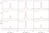 |
Fig. B.1. Observed lines of H2CCC in the 31-115 GHz domain toward TMC-1. The abscissa corresponds to the velocity of the cloud with respect to the Local Standard of Rest (vLSR). The ordinate is the antenna temperature corrected for atmospheric and telescope losses in mK. The spectral resolution is 38 kHz below 50 GHz and 48 kHz above. Derived line parameters are given in Table B.2. The red lines show the computed synthetic spectra for the lines of H2CCC (see text). The lines in the left column correspond to para lines of H2CCC, while those of the central and right columns correspond to transitions of the ortho species. The adopted frequencies are those of the CDMS catalog (Müller et al. 2005) and are given in Table B.2. |
Line parameters of the observed transitions of H2CCCH+ in TMC-1.
Line parameters of the observed transitions of H2CCC in TMC-1.
All Tables
Ground state rotational transition frequencies of H2CCCH+, determined by laboratory and astronomical detections.
Calculated and experimental spectroscopic parameters of H2CCC and H2CCCH+ (in MHz). Equilibrium rotational constants calculated at the ae-CCSD(T)/cc-pwCVQZ level of theory; zero-point vibrational corrections ΔA0, ΔB0, ΔC0; and centrifugal distortion constants calculated at the fc-CCSD(T)/ANO1 level. Best theoretical estimates for the rotational and centrifugal distortion constants X of H2CCCH+ are estimated as (i.e., using isoelectronic H2CCC as a calibrator).
All Figures
|
Fig. 1. Pure rotational transition ( |
| In the text | |
|
Fig. 2. Lines of H2CCCH+ observed in the 31–115 GHz domain toward TMC-1. The abscissa corresponds to the rest frequency in MHz. The ordinate is the antenna temperature corrected for atmospheric and telescope losses in mK. The spectral resolution is 38 kHz below 50 GHz and 48 kHz above. The line parameters are given in Table B.1. The red lines show the computed synthetic spectra (see text). |
| In the text | |
|
Fig. 3. Abundances of C3, C3H+, H2CCC, and H2CCCH+ as a function of time predicted by our model (continuous lines). The horizontal colored areas represent the observations in TMC-1 assuming an uncertainty of 3 on the measurements (Cernicharo et al. 2022 for C3H+ and this work for H2CCCH+). Dashed lines: Same, but with a threefold decrease in the H2 + C3H+ and a fivefold increase in the H2CCCH+ + e− rate coefficients. The vertical gray area represents the values given by the most probable chemical age for TMC-1, due to the better agreement between calculations and observations for 67 key species. |
| In the text | |
|
Fig. B.1. Observed lines of H2CCC in the 31-115 GHz domain toward TMC-1. The abscissa corresponds to the velocity of the cloud with respect to the Local Standard of Rest (vLSR). The ordinate is the antenna temperature corrected for atmospheric and telescope losses in mK. The spectral resolution is 38 kHz below 50 GHz and 48 kHz above. Derived line parameters are given in Table B.2. The red lines show the computed synthetic spectra for the lines of H2CCC (see text). The lines in the left column correspond to para lines of H2CCC, while those of the central and right columns correspond to transitions of the ortho species. The adopted frequencies are those of the CDMS catalog (Müller et al. 2005) and are given in Table B.2. |
| In the text | |
Current usage metrics show cumulative count of Article Views (full-text article views including HTML views, PDF and ePub downloads, according to the available data) and Abstracts Views on Vision4Press platform.
Data correspond to usage on the plateform after 2015. The current usage metrics is available 48-96 hours after online publication and is updated daily on week days.
Initial download of the metrics may take a while.