| Issue |
A&A
Volume 676, August 2023
|
|
|---|---|---|
| Article Number | A14 | |
| Number of page(s) | 11 | |
| Section | Stellar atmospheres | |
| DOI | https://doi.org/10.1051/0004-6361/202346470 | |
| Published online | 27 July 2023 | |
Complete X-ray census of M dwarfs in the solar neighborhood
I. GJ 745 AB: Coronal-hole stars in the 10 pc sample
1
Institut für Astronomie und Astrophysik, Eberhard-Karls Universität Tübingen,
Sand 1,
72076
Tübingen, Germany
e-mail: caramazza@astro.uni-tuebingen.de
2
INAF–Osservatorio Astronomico di Palermo,
Piazza del Parlamento 1,
90134
Palermo, Italy
3
University of Vienna, Department of Astrophysics,
Türkenschanzstrasse 17,
1180
Vienna, Austria
4
Leibniz Institute for Astrophysics Potsdam (AIP),
An der Sternwarte 16,
14482
Potsdam, Germany
5
Universität Potsdam, Institut für Physik und Astronomie,
Karl-Liebknecht-Straße 24/25,
14476
Potsdam, Germany
Received:
21
March
2023
Accepted:
24
May
2023
Context. X-ray emission is the most sensitive diagnostic of magnetic activity in M dwarfs and, hence, of the dynamo in low-mass stars. Moreover it is crucial for quantifying the influence of the stellar irradiation on the evolution of planet atmospheres.
Aims. We have embarked in a systematic study of the X-ray emission in a volume-limited sample of M dwarf stars to explore the full range of activity levels present in their coronae. We look to obtain a better understanding of the conditions in their outer atmospheres and their possible impact on the circumstellar environment.
Methods. Based on a recent catalog of Gaia objects within 10 pc from the Sun, we identified all its stars with spectral types between M0 and M4 and we carried out a systematic search for X-ray measurements of this sample. To this end, we used both archival data from ROSAT, XMM-Newton, and the ROentgen Survey with an Imaging Telescope Array (eROSITA) on board the Russian Spektrum-Roentgen-Gamma mission, as well as our own dedicated XMM-Newton observations. To make inferences on the properties of the M dwarf corona, we compared the range of their observed X-ray emission levels to the flux radiated by the Sun from different types of magnetic structures: coronal holes, background corona, active regions, and cores of active regions. In this work, we focus on the properties of stars with the faintest X-ray emission.
Results. At the current state of our project, with more than 90% of the 10 pc M dwarf sample observed in the X-ray, there is only one star that has had no detections: GJ 745 A. With an upper limit luminosity of log Lx (erg s−1) < 25.4 and an X-ray surface flux of log FX,SURF (erg cm−2 s−1) < 3.6, GJ 745 A defines the lower boundary of the X-ray emission level for M dwarfs. Together with its proper motion companion (GJ 745 B), it is the only star in this volume-complete sample located in the range of X-ray surface flux that corresponds to the faintest solar coronal structures, namely: coronal holes. The fact that the ultra-low X-ray emission level of GJ 745 B (log Lx (erg s−1) = 25.6 and log FX,SURF (erg cm−2 s−1) = 3.8) is entirely attributed to flaring activity indicates that while its corona is dominated by “holes,” at least one magnetically active structure is present. This structure determines the total X-ray brightness and the coronal temperature of the star.
Key words: X-rays: stars / stars: activity / stars: coronae / stars: low-mass
© The Authors 2023
 Open Access article, published by EDP Sciences, under the terms of the Creative Commons Attribution License (https://creativecommons.org/licenses/by/4.0), which permits unrestricted use, distribution, and reproduction in any medium, provided the original work is properly cited.
This article is published in open access under the Subscribe to Open model. Subscribe to A&A to support open access publication.
1 Introduction
M dwarfs are the most abundant stars in the Galaxy (Chabrier 2001). They also constitute the majority of the hosts of small, rocky planets (Howard et al. 2012), with estimates for the occurrence rate for Earth-like planets among early-M dwarfs ranging from 0.10 to 0.85 (e.g., Dressing & Charbonneau 2013; Pinamonti et al. 2022) and up to ≈25% of these planets being considered habitable (Pinamonti et al. 2022). The characterization of the M dwarf population is therefore of great importance to our understanding of both stellar evolution and the variety of exoplanet systems.
One piece in this puzzle is the high-energy emission coming from the stellar corona. In analogy with our Sun, the outer atmosphere of M dwarfs is considered to be heated by magnetic processes to temperatures above a million Kelvin that provide thermal emission in the UV and X-ray regime. X-ray emission is the most sensitive tracer for magnetic activity in M dwarf stars (Stelzer et al. 2013). The stellar dynamo that underlies these high-energy phenomena is driven by convection and (differential) rotation (Parker 1955, 1975). Both these parameters change across stellar mass and evolution, leading to a broad range of activity levels at given mass or age. Despite the existence of numerous studies of the subject (Pallavicini et al. 1981; Barbera et al. 1993; Fleming et al. 1995; Schmitt 1997; Fleming 1998; Marino et al. 2000), the full range of activity levels exhibited by low-mass stars has not yet been fully explored. The key to solving this problem are volume-limited samples.
X-ray luminosity functions for volume-limited samples of field dwarf stars have previously been presented by Schmitt et al. (1995) and Schmitt & Liefke (2004) based on ROSAT observations. The latter study comprised 37 stars with spectral types (SpT) M0…M4 within 6 pc. Since then, astrometric surveys have provided updates to the census of X-ray properties of the solar neighborhood. Stelzer et al. (2013) used the SUPERBLINK proper motion survey by Lépine & Gaidos (2011) to study the X-ray emission of nearby M dwarfs. Complementing ROSAT all-sky survey data with archival (serendipitous) XMM-Newton observations, it was found that ~40% of the M dwarfs within 10 pc of the Sun still had no sensitive limit on their X-ray luminosities. This has led us to embark into a dedicated XMM-Newton program to complete the 10 pc M dwarf X-ray luminosity function. In the meantime, improved astrometry has been provided through Gaia and a new census of nearby stars was published, known as “The 10 parsec sample in the Gaia era” (Reylé et al. 2021). We have used this updated 10 pc sample as a basis of our effort to provide an unbiased characterization of M dwarfs in the X-ray band.
With a systematic compilation from X-ray archives integrated by our dedicated observations to complete the M dwarf 10 pc X-ray census we are able to probe the full range of X-ray luminosities (Lx) present in early-M dwarf stars (spectral type M0–M4) for the first time. We find that their X-ray activity levels span three orders of magnitude, from the canonical saturation level of log (Lx/Lbol ≈ −3) or surface flux log FX,SURF (erg cm−2 s−1) ≈ 7, and higher during flares, to log FX,SURF (erg cm−2 s−1) ≈ 4. Remarkably, there is one star in the 10 pc sample, the binary GJ 745 AB, that appears to have an X-ray emission level significantly below this lower bound. Assuming that M dwarf coronae are composed of the same types of magnetic structures as the Sun, the only feature that can explain such low-level X-ray emission are coronal holes (CH). Coronal holes are regions of the solar corona characterized by low density plasma associated with open magnetic field structures that expand out into interplanetary space. They appear like X-ray darker areas in the corona of our Sun, but they show a nonzero emission and display a typical temperature Tx,CH ≈ 1MK (Cranmer 2009). Schmitt (1997) and Schmitt (2012),in their pursuit of the maximum and minimum value of the surface X-ray flux for solar-like stars, suggested that the expected minimum surface flux is expected when the stellar corona is completely covered by CHs, while the maximum is when it is covered by active regions. In this article, we focus on the X-ray properties of the two components of the ultra-low activity binary star GJ 745 AB in the context of the 10 pc sample of M dwarfs. In Sect. 2, we describe the new catalog of stars within 10 pc by Reylé et al. (2021) and how we extracted our volume-complete M dwarf sample from that work. In Sect. 3, we present our X-ray database and analysis. In Sect. 4, we discuss the stars of our catalog that have a coronal surface flux low enough that we could envision their corona to be completely covered by coronal holes.
2 The M10pc-Gaia sample
We constructed a volume-complete sample of M dwarfs with spectral type (SpT) from M0 to M4 based on the 10 pc-catalog published by Reylé et al. (2021). We restricted the sample to early M-type dwarfs because our study is aimed at compiling a sensitive X-ray census of the volume-limited sample. Since X-ray emission drops with later SpT most M dwarfs beyond M4 (even those at very close distances) are still out of reach for a systematic survey with current X-ray instrumentation that would require prohibitively long exposure times.
The Reylé et al. (2021) catalog includes 560 objects that were extracted from the SIMBAD database1 (Wenger et al. 2000) with the criterion of having a parallax larger than 100 mas. Among these, 346 objects have Gaia photometry. In Fig. 1, we visualize this sample in the Gaia color-magnitude diagram.
In the first phase of the sample downselection, we discarded all stars with Gaia GBP ≥ 20.3 mag since for these faint objects the flux in Gaia’s blue photometer is overestimated, leading to an unphysical turnaround of the lower main-sequence that is seen in Fig. 1 (see discussion in Riello et al. 2021). We then selected all stars that have GBP – GRP color corresponding to M0–M4 SpT. We performed the association of Gaia color with SpT using the table from Pecaut & Mamajek (2013), integrated with Gaia photometry and maintained by Eric Mamajek2.
The sample selected that way consists of 150 stars. This number is in reasonable agreement with the extrapolation from the sample presented by Schmitt & Liefke (2004) for a volume of 6 pc radius. These authors counted 37 stars of spectral type M0…M4, while our M10PC-GAIA SAMPLE counts 43 stars within a 6 pc distance. This difference is probably to be attributed to the different ways in which the databases were collected, spectral types assigned, and multiplicity treated. Reylé et al. (2021) consider their catalog to be complete down to SpT Y2. In fact, as can be seen from Fig. 1, the faintest stars in the M 10PC-GAIA SAMPLE have G ≈ 13 mag, many orders of magnitude above the Gaia sensitivity limit.
Knowledge of the fundamental parameters of the stars is essential for the interpretation of the X-ray data. In particular, the stellar radius (R*) is required to determine the X-ray surface flux, which is the most useful parameter for comparing the activity levels for a range of stars. We calculated R* from KS magnitudes reported in Reylé et al. (2021), adopting the empirical relation by Mann et al. (2015).
Another essential parameter needed to achieve a better understanding of our M dwarf sample is the stellar metallicity. Therefore, we collected metallicity values [Fe/H] from the literature for the M 10PC-GAIA stars. Marfil et al. (2021) reported metallicities for a sample of 343 M dwarfs observed with CARMENES, of which 76 stars are in common with the M 10PC-GAIA SAMPLE. GJ 745 AB, the binary system we focus on in the following, belongs to this group. Here, we use their metallicity values obtained in the STEPARSYN run, whereby all parameters were allowed to vary. Measurements of [Fe/H] for the remaining stars were collected from Birky et al. (2020), Maldonado et al. (2019), Mann et al. (2019), Gáspár et al. (2016), Newton et al. (2014), Neves et al. (2013) and Rojas-Ayala et al. (2012). Finally, we adopted the metallicity from the Tycho-2 catalog (Ammons et al. 2006) for one additional binary pair. In total, we found [Fe/H] values for 135 of the 150 stars.
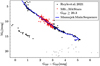 |
Fig. 1 Gaia color–magnitude diagram for the 10 pc census from Reylé et al. (2021). The stars with unreliable GBP magnitudes are shown in gray and the selected M10PC-Gaia SAMPLE (restricted to SpT M0…M4) is highlighted in red. Superposed is the main-sequence from E. Mamajek’s table (see https://www.pas.rochester.edu/~emamajek/EEM_dwarf_UBVIJHK_colors_Teff.txt). |
3 X-ray data base and analysis
We compiled an X-ray catalog for the 10PC-GAIA SAMPLE using both archival data and observations obtained by us through dedicated XMM-Newton pointings with the purpose of completing the X-ray census of early-M dwarfs within 10 pc of the Sun. The archival data comes from ROSAT/PSPC (Briel & Pfeffermann 1986) observations both during the all-sky survey phase and the subsequent pointed phase, from the all-sky survey of the extended ROentgen Survey with an Imaging Telescope Array (eROSITA; Predehl et al. 2021) on the Spectrum-Roentgen-Gamma (SRG) mission and from pointed XMM-Newton observations, as explained in Sects. 3.1 to 3.4. Targets that at the beginning of the project had no X-ray detections in any of these databases are observed in the framework of an XMM-Newton FULFIL program (PI Stelzer Obs ID 084084, 086030).
The full X-ray catalog will be published after the X-ray census is completed. To date, we still need to observe 9 out of the 150 M dwarfs within 10 pc of the Sun. These are part of an XMM-Newton/AO22 campaign (PI Stelzer; ObsID 092126) in continuation of the above mentioned FULFIL program that started in AO18. Here, we describe how we compiled the X-ray data base and how we extracted the basic parameter: a homogeneously determined X-ray flux for all sample stars.
The most delicate step in the construction of a homogeneous X-ray catalog is the calculation of the flux from the count rate for observations acquired with instruments that cover different energy bands, here XMM-Newton, eROSITA, and ROSAT. Therefore, we computed the X-ray fluxes for the observations of each database separately, with an instrument-specific rate-to-flux conversion factor (CF). All fluxes were calculated for the 0.1–2.4 keV ROSAT energy band, which is the band that is most common in the literature. Also, this energy band has been used in the construction of empirical relations between X-ray and EUV flux and luminosity (e.g., Sanz-Forcada et al. 2011; Chadney et al. 2015). Thus, it allows for the most direct conversion between the two energy bands. We note that to cover the ROSAT band, we had to slightly extrapolate the energy range at the low end covered by the other X-ray instruments, that is, by 0.1 keV for eROSITA and XMM-Newton. Since our flux calculation is based on a given spectral model, this means that we implicitly assume that at the low-energy end, there is no additional spectral component contribution. In Table 1, we list the CF that we used for the three instruments to calculate a homogeneous X-ray flux in the ROSAT band. Explanations on how we derived these values are found in the rest of this section.
3.1 ROSAT All-Sky Survey
We extracted data from the Second ROSAT All-Sky Survey Point Source Catalog (2RXS; Boller et al. 2016), which is a revised version of the earlier bright (Voges et al. 1999) and faint (Voges et al. 2000) source catalogs. It tabulates count rates in the 0.1–2.4 keV band for more than 130 000 X-ray sources distributed over the whole sky.
To match the M 10PC-GAIA SAMPLE with 2RXS we followed the procedure of Stelzer et al. (2013). We first extrapolated the star coordinates reported by Reylé et al. (2021) back to October 1, 1990, a date representative for the observing epoch of the RASS which lasted from August to December 1990. Then, we performed a cross-match with a radius of 40″ (Neuhaeuser et al. 1995), finding that 86 stars of our sample were detected in RASS.
For the conversion of the 2 RXS count rates to fluxes, as the 0.1–2.4 keV conversion factor we used the value of CFROSAT = 5.77 × 10⁻¹² erg cm−2 cts−1 determined by Magaudda et al. (2020), with the Mission Count Rate Simulator WebPIMMS3 for a 1T-APEC model with a temperature of kT = 0.5 keV. This spectral model is the average of the best fit parameters obtained for XMM-Newton and Chandra spectra of Magaudda et al. (2020) M dwarf sample.
Conversion factor between count rate measured with different X-ray instruments and flux in the 0.1–2.4 keV ROSAT band.
3.2 eROSITA All-Sky Survey
We used the merged catalog of the first four eROSITA all-sky surveys (eRASS:4) in the version available to the eROSITA_DE consortium in October 20224. The eROSITA catalogs available to us have been produced at Max-Planck Institut für extraterrestrische Physik and they comprise data from the western galactic hemisphere (l ≥ 180°) which is the half of the sky with german data rights. Before the match with a radius of 30″ we have translated the coordinates of the M 10PC-GAIA stars to the mean observing date of the four eRASS surveys, 15 December 2020. None of the sample stars has a proper motion as high as to be able to move outside the 30″ match radius within one year, namely the time difference between the above mentioned mean eRASS date and the beginning of the first and the end of the forth survey. With this catalog match we found 69 eRASS detections among the M10PC-GAIA stars.
The eRASS:4 catalog holds count rates in a single energy band ranging from 0.2–2.3 keV. We converted them into flux in the ROSAT band by means of the conversion factor CFeRASS = 8.78 × 10⁻¹³ erg cm−2 cts−1. We derived this value from a combination of one and two temperatures APEC models for a sample of early M dwarf stars studied in Magaudda et al. (2022). The CFeRASS of this work appears slightly higher than the value published in Magaudda et al. (2022) because that study adopted the eROSITA broad band (0.2–5.0 keV), while we limited our analysis to the energy band of ROSAT (0.1–2.4 keV).
3.3 ROSAT pointed catalog
In our search for M 10PC-GAIA stars in pointed ROSAT observations, we cross-matched their coordinates with those in the Second ROSAT Source Catalog of Pointed Observations (Rosat 2000) which provides count rates in the 0.1–2.4 keV band from stars detected in pointed ROSAT/PSPC observations.
We proceeded with the propagation of the coordinates to the epoch of the X-ray data analogously to the steps discussed above for 2 RXS and eRASS:4. The difference is that the 2 RXP data is spread over a much longer time range (about 7 yr). Therefore, a mean proper motion correction may not yield a position at the time of the ROSAT observation that is accurate enough to retrieve the X-ray counterparts for all stars. Instead, individual proper motion corrections must be applied for each target to its ROSAT observing date. Since we did not know this date a priori, we started with an initially very large match radius of 260″. This value is motivated by the maximum proper motion of our stars between the year 1991, namely, the epoch of the first pointed ROSAT observations and their Gaia position.
The value of CFROSAT = 5.77 × 10⁻¹² erg cm−2 cts−1 that was used for the RASS detections (see Sect. 3.1) was used here to obtain the 0.1–2.4 keV fluxes from the count rates listed in 2 RXP.
3.4 XMM-Newton
To find targets detected with XMM-Newton we have searched the 4XMM-DR11 catalog (Webb et al. 2020) and, for more recent observations, we consulted the XMM-Newton archive5 directly. For simplicity, we made use only of the most sensitive of the EPIC instruments, the pn CCDs.
Similar to the case of the pointed ROSAT catalog, since there are up to 16 yr between the epochs of the XMM-Newton observations in 4XMM-DR11 and of Gaia-eDR3, we had to perform individual proper motion corrections for our target stars. The initial match radius we used was 180″, motivated by the maximum proper motion expected for any of our targets within the maximum possible time difference of 16 yr. The coordinates of the stars that present one or more XMM-Newton counterparts for this large search radius were then propagated to the epoch of the specific XMM-Newton observation. The subsequent refined cross-match was performed with a radius of 15″. In this way, we found that 28 stars of the M 10PC-GAIA SAMPLE have at least one detection in the 4XMM-DR11 catalog.
The XMM-Newton archive holds more recent observations than 4XMM-DR11 for an additional eight M 10PC-GAIA stars from our dedicated XMM-Newton FULFIL survey. For these observations, we used the standard SAS pipeline for the source detection and the determination of the count rate. X-ray counterparts were then identified by means of a cross-match, with a radius of 15″, between the position of the detected X-ray sources and those of the Gaia position propagated to the date of the XMM-Newton observation.
One star required a special treatment for its detection: GJ 643 was observed with XMM-Newton, but it is located in the wings of the EPIC/pn point spread function (PSF) of the much brighter star GJ 644, which is also a member of the M 10PC-GAIA SAMPLE. With a special background subtraction and thanks to a flare event on GJ 643, we managed to detect the star in spite of the fact that the noise by far exceeds the signal. The analysis of the EPIC/pn data for this object is detailed in Appendix A.
For all M10PC-GAIA stars observed with XMM-Newton, whether extracted from the 4XMM-DR11 catalog or directly from the archive, we followed Magaudda et al. (2020) and converted their EPIC/pn count rates in the full 0.2–12 keV energy band into flux in the ROSAT band with the conversion factor value of CFXMM = 1.38 × 10⁻¹² erg cm−2 cts−1, calculated with WebPIMMS for a 1T-APEC model with a temperature of kT = 0.5 keV.
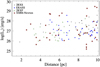 |
Fig. 2 X-ray luminosity versus distance for the M 10PC-GAIA SAMPLE. For stars detected more than once, the Lx value from the deepest survey was used in the order explained in the text. Among all the other stars, only one has remained undetected, namely, GJ 745 A, which has an upper limit indicated by the downward pointing arrow. |
3.5 Summary of X-ray detections
Many stars have more than one X-ray detection, which allows for a variability study that we defer to a future work. For the current study, we focused on the overall range of X-ray emission levels of early-M dwarfs. Figure 2 shows the X-ray luminosities for the whole M 10PC-GAIA sample. Since some stars have been observed more than once, we plot in this figure the X-ray detection from the deepest data overall: XMM-Newton, 2RXP, eRASS and RASS (in this order). Specifically, Fig. 2 presents 37 stars detected with XMM-Newton, 28 from 2RXP, along with an additional 38 stars from eRASS:4 and 30 from 2RXS.
Besides the nine stars that have not been observed thus far and that are part of our ongoing observational campaign, there is just one object, GJ 745 A, that has deep X-ray data from our dedicated XMM-Newton survey and that has not yet been detected. In Sect. 3.6, we explain how we extracted the upper limit to its X-ray emission.
3.6 A very deep X-ray upper limit for GJ 745 A
GJ 745 A is part of a multiple system together with GJ 745 B, its proper motion companion. The system was observed twice with XMM-Newton. The first observation was taken on Sept. 27–28 2019 (Obs ID: 0840843401) for 32.4 ks, with GJ 745 B as main target. One year later, on Sept. 20–21 2020, GJ 745 A was observed for 31.7 ks in a dedicated observation (Obs ID: 0860303001). With a separation of 114.06″ (Andrews et al. 2017), the two components of GJ 745 are clearly resolved with XMM-Newton.
We analyzed both XMM-Newton EPIC/pn observations using the Science Analysis Software (SAS) version 19.1.0 developed for the satellite. By examining the high energy events (≥10 keV) across the full EPIC/pn detector, we excluded the time intervals affected by the solar particle background. We note that the latest observation (0860303001) is affected by a large background event that reduced the good time intervals and, consequently, the exposure time by about 50%. We filtered the data for pixel patterns (0 ≤ pattern ≤ 12), quality flag (flag = 0), and events channels (PI ≥ 150). The source detection was performed in three energy bands: 0.2–0.5 keV (S), 0.5–1.0 keV (M), and 1.0–2.0 keV (H).
GJ 745 A was not detected in either of the two observations. Making use of the SAS tool ESENSMAP, we calculated the sensitivity map in the 0.2–12.0 keV band and derived the two upper limits at the Gaia position of the star propagated to the date of each observation. These two values are reported in Table 2. The difference of the exposure time and the different level of background of the two observations leads to different upper limit count rates. In the following, we use the lower, (i.e., more sensitive) value (0.0020 cts s−1) as the upper limit count rate for GJ 745 A.
Converting the count rate to luminosity in the 0.1–2.4 keV band (as explained in Sect. 3.4), we obtained log Lx (erg s−1) < 25.4. For the star’s stellar radius of 0.34 R⊙ the X-ray surface flux is log FX,SURF < 3.55 erg cm−2 s−1. Here, we have used the conversion factor that applies for a coronal temperature of 0.5 keV. In Sect. 4, we show that the faint X-ray emission level of GJ 745 A is consistent with the emission of solar coronal holes, which have lower temperatures. If we assume that the temperature in GJ 745 A’s corona is 0.1 keV, the resulting X-ray surface flux would be log FX,SURF < 3.74 erg cm−2 s−1.
Upper limit count rates and effective exposure time after removal high-background time intervals for GJ 745 A during the two XMM-Newton observations.
4 Discussion
Figure 2 shows a remarkable distribution for the Lx values in the M 10PC-GAIA SAMPLE. Next to a scatter of the detections by about two orders of magnitude a lower envelope is seen that is located at approximately log Lx (erg s−1) = 26. This value shows no obvious dependence on distance, indicating that there is no sensitivity-related X-ray detection bias. Leaving aside the nine stars that still need to be observed in our XMM-Newton program, the M 10PC-GAIA SAMPLE is the first truly volume-complete M dwarf sample in both the optical and X-ray.
The most universal diagnostic for coronal brightness is the surface X-ray flux, FX,SURF, since it is independent of the stellar radius. In Fig. 3, we show FX,SURF versus Gaia color for the M 10PC-GAIA SAMPLE. In the solar corona, individual types of magnetic structures characterized by different levels of X-ray brightness can be distinguished in the images and their emitted flux can be quantified. Such studies were carried out as part of the project titled The Sun as an X-ray star (see Orlando et al. 2004). From a comparison of the observed range in the X-ray emission level of a stellar sample with these solar structures, it is therefore possible to estimate which types of magnetically active regions dominate in the coronae of the stars.
4.1 The X-ray emission from solar coronal structures
Within The Sun as an X-ray star project, Yohkoh observations have been used to quantify the emission measure distributions of different types of magnetic structures in the solar corona (Orlando et al. 2000b, 2001; Peres et al. 2000; Reale et al. 2001). These structures are defined by their surface brightness, in increasing order from: the background corona (BKC) via active regions (AR) to cores of active regions (CO) (see Orlando et al. 2001). For our purposes, the Yohkoh data from July 1996 was used when there was only one active region (emerged on July 4) on the Sun (see Orlando et al. 2004) and the range of X-ray fluxes for the different types of regions derived from these data are listed in Table 3. In Fig. 3, we overlay the range of BKC, AR, and CO as colored areas. Clearly, the possibility that on some other date the Sun displayed regions with slightly different properties cannot be excluded, but the ranges given in Table 3 should be approximately representative for each type of magnetic solar structure.
The lowest expected X-ray emission level of a late-type star is that of a corona characterized by open field lines where hot plasma is escaping into space. On the Sun, this configuration corresponds to the so-called coronal holes. The surface flux of (solar) coronal holes in the 0.1–2.4 keV ROSAT band has been computed by Schmitt (2012) for a range of temperatures observed in coronal holes on the Sun. In Fig. 3, we include the range of X-ray surface flux values for a solar coronal hole corresponding to plasma temperatures from 1 MK (upper bound of the colored stripe) up to 2 MK (lower bound of the stripe). The CH flux corresponds, as predicted, to the lowest X-ray emission levels observed on the Sun, but the CH region shows some overlap with the BKC. The BKC corresponds to faint and diffuse regions with pixels with a good signal-to-noise ratio (i.e., S/N with more than ten photons per pixel; see Fig. 12 in Orlando et al. 2000a) and surface intensity below a threshold to exclude ARs and COs (see Fig. 2 in Orlando et al. 2001). This selection criterion effectively eliminates regions with very low emission (i.e., pixels with fewer than ten photons), resulting in the exclusion of the weakest parts of CHs. Consequently, there is a significant difference in the flux level between BKC and CHs.
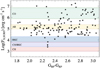 |
Fig. 3 X-ray surface flux versus Gaia GBP – GRP color for the M 10PC-GAIA SAMPLE. Each star is represented by its mean X-ray emission level from our multi-mission data base. Colored areas mark the range of surface flux for four typical non-flaring magnetic regions in the solar corona, coronal holes (CH), background corona (BKC), active regions (AR), and cores of active regions (CO); see Table 3. The flux ranges of the BKC and CH overlap. Only two stars are located within or in the immediate vicinity of the “coronal hole” area: the binary pair GJ 745 A and B, where the upper limit is given for the A component of the system. |
X-ray surface fluxes for magnetic structures (BKC, AR, and CO) in the corona of the Sun obtained from Yohkoh data collected in July 1996 (during a minimum in the solar cycle) within the Sun as an X-ray star framework.
Activity-related properties of CH M dwarfs in the M 10PC-GAIA SAMPLE.
4.2 Coronal hole-like M dwarfs
Several nearby M dwarfs appear to be very X-ray quiet as inferred from the comparison with the solar data in Fig. 3. However, only two stars have X-ray surface fluxes as low as solar CHs. This is the binary pair GJ 745 A and B, with the primary component being the only star in our sample that is not detected. If the lowest X-ray emission level of M dwarfs is represented by the flux of a solar CH, these stars might thus be completely covered with CHs. Since their flux lies in the overlapping locus between the CH and BKC, their emission could also be explained with a quiet corona without active regions. A more realistic scenario may correspond to a combination between the CH and BKC, although a small contribution by brighter magnetic structures (AR and CO) cannot be excluded. Analogously, for the more active stars it is not possible to clearly associate their X-ray emission with one type of magnetic structure since any real stellar corona, just as our Sun, can be expected to be composed of a mixture of CH, BKC, AR, and CO (with occasionally flaring structures), as well as the relative covering fraction for each of these structures cannot be quantified with a simple flux measurement.
Although the X-ray emission of GJ 745 can be explained by either the CH or BKC alone, they are the only stars of our sample consistent with a CH-like corona. Therefore, we focus in the following on a description where the corona is a combination of some area fraction of BKC, AR, or CO with the remaining larger part covered with CHs, that is:
 (1)
(1)
Here, REG stands for one of the solar magnetic regions (BKC, AR, or CO) and f is the filling factor that is a percentage area coverage.
The two components of the GJ 745 binary are twins, with equal radii (R* = 0.34 R⊙) and masses (M* = 0.34 M⊙). The apparently X-ray dark star, GJ 745 A, has an upper limit of log Fx,suRF,GJ745A(erg cm−2s−1) < 3.55, and its companion, GJ 745 B, is a very weak X-ray source with log Fx,SURF,GJ745B(erg cm−2s−1) = 3.82 (see Table 4). For our evaluation of Eq. (1), we consider for CHs the minimum flux (lower bound in Fig. 3) of 〈FCHerg cm−2 s−1〉 = 103.0 and for REG, we used the minimum values from Table 3. In this way, we obtained an upper limit to the flux contribution from the brighter region, namely, REG. With this approach, the observed X-ray upper limit for GJ 745 A can be explained with a corona covered in large part with CHs, except for 2.7% of AR or 0.3% CO. On the other hand, assuming the star to be completely covered with the BKC at the minimum solar flux value, the resulting luminosity would be below the observed X-ray upper limit and, hence, a BKC-like corona is also compatible with the observation of GJ 745 A. However, if we replace the minimum solar BKC flux by the average, the scenario is that of a star with dominating emission of CH and a BKC filling factor area of 21.8%.
The time-averaged X-ray surface flux of GJ 745 B, like that of its companion, is compatible with a scenario where the emission is entirely explained by a BKC. A combination of the CH+BKC, both at the minimum of the solar values is not able to explain the observed flux of GJ 745 B. If, instead, we consider the star to be dominated by the CH and BKC at the mean solar flux, we obtained a BKC filling factor of 48%. Another scenario would be that of 6.0% of the corona covered with solar-like AR and the rest with CH. Replacing the AR with CO we find for GJ 745 B a maximum filling factor with CO of 0.72%. As we show below in Sect. 4.2.2, GJ 745 B underwent a flare during the XMM-Newton observation. Since flares on the Sun take place in the COs of ARs the presence of an erupting CO on the corona of GJ 745 B is plausible.
4.2.1 Coronal brightness and temperature
For GJ 745 A the upper limit does not provide us any information on its coronal temperature. However its companion GJ 745 B was detected with 49 ± 9 EPIC/pn counts from ObsID 0840843401. The collected counts are too few for a spectral fit, therefore we studied its spectral shape through hardness ratios.
For the hardness ratio analysis we use standard XMM-Newton energy bands, 0.2–0.5 keV, 0.5–1.0 keV and 1.0–2.0 keV; henceforth named S, M, and H for the soft, medium, and hard part of the X-ray spectrum. The hardness ratios are defined as HR1 = (RateM – RateS)/(RateM + RateS) and HR2 = (RateH – RateM)/(RateH + RateM), where Rate is the net source count rate resulting from the source detection process in the respective energy band.
Figure 4 shows the hardness ratio plot for all M10PC-GAIA SAMPLE stars observed and detected with XMM-Newton, including the CH star GJ 745 B which is highlighted with a blue colored plotting symbol. Superposed on the data is a grid calculated for a 2T-APEC model from a simulated XMM-Newton spectrum using the EPIC/pn response matrix and the exposure time of the observation of GJ 745 B amounting to 32 ks. The low-temperature component is fixed on kT1 = 0.1 keV and the second component, kT2, varies from 0.1 to 0.9 keV in steps of 0.2 keV. The coronal abundance of both spectral components was set to 0.3 times the solar value as typical for late-type stars (e.g., Favata et al. 2000; van den Besselaar et al. 2003; Robrade & Schmitt 2005; Maggio et al. 2007) using the library from Asplund et al. (2009). A third parameter is the ratio of the two emission measures (EM2/EM1). In a collisionally ionized plasma the EM is a measure for the X-ray emitting power. It is given by the volume integral of the product of the densities of electrons and ions at a given temperature, where the latter ones are related to the hydrogen density through the elemental abundance. Since HR is a normalized quantity, the absolute values for the two EMs do not play a role here. We computed our model for values of the ratio of the emission measures varying from 0.2 to 12.0, namely, this is where the softer temperature component is responsible for most of the emission to where the harder component dominates. From the comparison of this model grid with the data, we see that all stars have negative HR2, indicating an only weak contribution from emission at energies >1 keV, namely, in band H. This is consistent with the uppermost value for kT2 in the grid of 0.9 keV. While in our sample there are stars with very soft emission, that is, HR1 < 0, for the majority of stars, the dominating emission is in band M. The empirical upper boundary of our sample in terms of HR1 is matched well by the model with EM2/EM1 = 2, but the stars with the highest values of HR1 require EM2/EM1 = 12, corresponding to coronae where the softer component is of little importance. We verified the negligible contribution of the soft component by comparing this model with the hardness ratios from a simulated 1T-APEC spectrum. This latter one, indeed, closely follows our upper boundary 2T-model (with EM2/EM1 = 12) which thus represents a point of saturation for our two-temperature grid.
Remarkably, GJ 745 B is located at the upper boundary in terms of EM2/EM1, presenting the highest value of HR1 in the whole sample. The model that best describes the hardness ratios of GJ 745 B is the one with kT1 = 0.1 keV, kT2 = 0.7 keV and EM2/EM1 = 12.0, yielding an emission measure weighted mean coronal temperature of 0.65 keV.
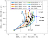 |
Fig. 4 Hardness ratios of the stars from the M 10PC-GAIA SAMPLE that are detected with XMM-Newton (filled black squares), with the CH star (in blue) highlighted. Superposed on the data is a grid of 2T-APEC models with a fixed kT1 at 0.1 keV, kT2 and EM2/EM1 ranging from 0.1 keV to 0.9 keV and 0.2 to 12, respectively (see Sect. 4.2.1 for more details). |
4.2.2 Flare on a coronal hole star
We extracted the EPIC/pn light curve of GJ 745 B for the same XMM-Newton energy band used for the hardness ratio (0.2–2.0 keV) and with a time bin size of 800 s (see Fig. 5). The source counts were extracted from a region of 30″ and the background from a region of 70″ radius. After background subtraction, the count rate in the light curve is consistent with a non-detection, except for the last hour of the observation, when the rate rises from ~0 cnt s−1 to ~0.015 cnt s−1. This evident flare is the likely explanation for the high coronal temperature identified in the hardness ratio analysis.
We computed the energy emitted during the flare (Eflare), adopting as the “quiescent” activity level the average count rate before the rise, amounting to 5.4 × 10⁻⁴ cnt s−1. This rate is represented by the red dashed line in Fig. 4 where we also show its standard deviation as red shaded area. We extracted the total flare counts by subtracting the quiescent rate from the rate of the last five bins, multiplying by the time bin size and summing over all elements. In this way, we found log Eflare (erg) = 29.72 ± 0.09 with the Gaia-DR2 distance (8.83 ± 0.01 pc) and the CF given in Sect. 3.4. Although this CF was computed for a slightly different energy band, it can be applied here because the time-averaged count rate in the light curve of Fig. 5 is consistent with the count rate listed in the 4XMM-DR11 catalog for the 0.2–12 keV band; hence, there is no significant emission outside the narrower energy range we used for the light curve. The flare peak luminosity extracted from the last four bins with the highest count rate is Lx,flare (erg s−1) = 26.2 ± 0.1 erg s−1. The pre-flare quiescent count rate, red dashed line in Fig. 5, is consistent with zero. Therefore, GJ 745 B is undetected outside the flare event. We extracted the upper limit from the sensitivity map for the out-of-flare time interval, finding Lx,quies (erg s−1) < 25.52.
Outside this flare event the star is undetected, which means that its emission state is similar to that of its sibling GJ 745 A. At first sight it seems remarkable to observe a flare on a star that is otherwise X-ray dark at the level of CH-emission. However, it is to be kept in mind that the emission we observe is averaged across all magnetic structures present on the stellar surface and, therefore, although most of the corona of GJ 745 B seems to be covered with X-ray dark CHs, a flare occurring in a single region capable to hold closed field lines has a great impact on the X-ray light curve and the coronal temperature (hardness ratio) of the star. In fact, above we have shown that the time-averaged X-ray luminosity of GJ 745 B can be explained if a minor fraction of its corona (0.72%) is covered with an eruptive solar-like CO.
By inference from our Sun, flares occur within COs. Assuming that the CO was already present before it erupted into a flare, a plausible description associates the “quiescent” corona of GJ 745 B (before the flare) with a superposition of a quiescent CO and CHs. Equation (1) applied to Lx,quies,GJ745B yields an upper limit to the CO filling factor of 0.5%. To estimate the filling factor of the flare we take the maximum of the surface fluxes of solar CO from Table 3 as a lower limit to the flux of the flare. The peak X-ray luminosity during the flare (logLx,flare (erg s−1) = 26.2) then yields a filling factor of this flaring structure of at least 0.3%.
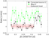 |
Fig. 5 Background-subtracted EPIC/pn light curve of GJ 745 B (black) and light curve of the background (green), both with a bin size of 800 s (see Sect. 4.2.1). We also show the quiescent rate with its standard deviation (red dashed line and shade, respectively) that we adopted for the calculation of the flare energy as explained in Sect. 4.2.2. The light curve is shorter than the nominal exposure time due to high and variable background at the end of the observation. |
4.2.3 Metallicity and space motion
In the search for a parameter that would distinguish the CH M dwarfs from the bulk of the M 110PC-GAIA SAMPLE we examined the metallicity from our compilation, described in Sect. 2. As can be seen from Fig. 6, it is indeed the case that GJ 745 A and B are also among the lowest metallicity stars in the M 10PC-GAIA SAMPLE. Yet there are some other sample members with even lower values of [Fe/H] reported in the literature but at the high end of the X-ray brightness distribution. These are EVLac, G19-7, and GJ 867.
Metallicity is difficult to measure in low-mass stars and, therefore, it has long been a missing piece in the evolutionary picture. Recently, Amard & Matt (2020) presented evolutionary calculations predicting that low-metallicity stars rotate faster at a given age, yet they have a higher Rossby number because their convective turnover times are smaller. We caution that their model is valid for solar-like stars. If this scenario also holds for M dwarfs and if magnetic activity is ruled by a Rossby number rather than rotation period alone, low-metallicity stars are expected to be less active than solar- or higher-metallicity stars. Newton et al. (2016, in their Fig. 10) have examined the relation between [Fe/H] and Prot and found “no clear trend” for a sample of nearly 450 M dwarfs. The lowest metallicities in their sample were, however, found at very slow rotators with rotation periods Prot ≈ 100 days. If the key parameter is R0 this does not contradict the expectation of lowered activity in low-metallicity stars. In the study of Newton et al. (2016), only two stars have a metallicity value that is as low as that of our CH stars.
We also computed the space motions of GJ 745 A and B using their Gaia coordinates, proper motions, parallaxes, and radial velocities. The result is given in Table 4. GJ 745 A and B are thin-disk objects, according to the Toomre diagram from Kirkpatrick et al. (2021).
4.2.4 Rotation
Available studies on the stellar rotation indicate that GJ 745 A and B are very slow rotators. Spectroscopic observations by, for instance, Delfosse et al. (1998), Browning et al. (2010) and Reiners et al. (2012) could only report upper limits on the rotational velocity υ sin i. The most recent measurement by Jeffers et al. (2018) with CARMENES resulted in υ sin i < 2 km s−1. Photometric studies using MEarth data (West et al. 2015; Newton et al. 2016) and a combination of MEarth and ASAS data (Díez Alonso et al. 2019) yielded no detections for the rotation period. In fact, the latter work reported a period of Prot = 3.8 ± 0.01 d for GJ 745 B, but with a high false alarm probability of 0.91%.
GJ 745 A and B were observed with the Transiting Exo-planet Survey Satellite (TESS) in sectors 40 and 54. We downloaded the 2-min cadence light curves from the MAST (Barbara A. Mikulski Archive for Space Telescopes) Portal. The search for the rotation period was carried out as explained by Stelzer et al. (2022a) using three different methods: the generalized Lomb–Scargle-Periodogram (GLS; Zechmeister & Kürster 2009), autocorrelation function, and sinefit. For each sector, we carried out individual searches for periods up to the duration of a TESS sector, which is about 27 days. All three methods for both stars in both sectors found signals with amplitudes that are between 3.5 and 18 times lower than the standard deviation of the light curves. Hence, we did not detect any rotation period for the two stars.
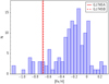 |
Fig. 6 Metallicity of the M 10PC-GAIA SAMPLE extracted from the literature cited in Sect. 4.2.3. The coronal hole stars are highlighted. |
4.2.5 Chromospheric activity
Reports on the chromospheric activity of GJ 745 A and B include Ha equivalent widths (EWs) of 0.06 Å for GJ 745 A (Newton et al. 2017) and around −0.1Å for GJ 745 A and B (Schöfer et al. 2019). Hence, only a weak Hα line is present meaning that GJ 745 A and B are inactive stars.
To compare the Hα EWs of GJ 745 A and B to all stars in the M10PC-GAIA SAMPLE we collected Hα EWs measurements from the literature. Gaidos et al. (2014) reported Hα EWs for 129 M dwarfs from our sample. When the data were available, we updated this table with more recent measurements from Newton et al. (2017), Schöfer et al. (2019), Medina et al. (2020) and Zhang et al. (2021). Finally, we added values from Gizis et al. (2002) and Houdebine (2012) for four additional stars. In total, we found Hα EWs for 136 of the 150 stars. The comparison with our full sample showed that GJ 745 A and B are typical for the low-activity stars in the M 10PC-GAIA SAMPLE. The comparison between the coronal and the chromospheric emission of the M 10PC-GAIA stars will be discussed in more detail in a future work.
5 Summary and conclusions
We have explored the X-ray emission levels of M dwarfs on the volume-limited sample within 10 pc. Comparison with the flux emitted by individual magnetic structures on the corona of the Sun shows that the full range covered by these solar regions, from emission brighter than the cores of active regions to the faint background Sun, is present in M dwarfs. The X-ray faintest M dwarfs comply with the faintest X-ray radiation of the Sun, suggesting that magnetic structures on M dwarf coronae are of the same nature as the ones observed on the Sun. Most notably, we have identified two stars that are fainter than even an hypothetical star that is entirely covered with an average solar BKC. The primary component of the common proper-motion binary, GJ 745 AB, is undetected at an X-ray flux level within the range displayed by solar CHs. Its companion is the faintest X-ray detected star in the whole M 10PC-GAIA SAMPLE and its X-ray surface flux is at the upper end of that of solar CHs. The flux of both components is compatible with a corona entirely covered by CHs or a BKC or a combinations of them: considering a dominating emission of CHs, the resulting filling factor of BKC is 21% for GJ 745 A, while for GJ 745 B is 48%. Another possible scenario is a corona covered by CHs, with a small fraction of ARs or even COs. In fact, our time-resolved analysis of GJ 745 B has demonstrated that the detection is owed to a flare, while the star is X-ray dark outside this event, just as its twin GJ 745 A. Specifically, we have computed a coronal filling factor with (flaring) CO of 0.3% for GJ 745 B as being consistent with its X-ray flux during the flare.
From this estimate for the CO filling factor, we can make inferences on the geometry of the flare. Assuming the 0.3% CO filling factor to be concentrated in a single CO, this structure has an area of 2 × 1019 cm2. However, it is likely that the flaring area was a fraction of the CO area but with a higher flux. As a template we make use of the X9 flare on the Sun analyzed by Reale et al. (2001) which covered an area of 3 × 1019 cm2 and its flux was log FX9,SURF (erg cm−2 s−1) = 7.93. A flare of the same flux combined with the rest of the corona of GJ 745 B being covered with CH is consistent with the observed X-ray flux of the star if the flare filling factor was 0.02%. We note that the solar X9 flare covered a similar area fraction, namely 0.05% of the solar surface. However, due to the smaller radius of GJ 745 B, 0.02% surface coverage corresponds to an area of only 1.8 × 1018 cm2. If we assume a loop of length, L, and width w ≈ 0.1L (White et al. 2002; Aschwanden & Peter 2017) this area translates into L ≈ 4 × 109 cm, which is comparable to the typical loop lengths observed on solar flares (see, e.g., Table 2 in Reale et al. 2001) and on the prototypical M dwarf flare star AD Leo (Stelzer et al. 2022b).
An empirical relation between X-ray temperature and surface flux for coronally active stars was presented in Johnstone & Güdel (2015). If we assume that this relation holds also for individual flare events, for the solar X9 flare from Reale et al. (2001), a coronal temperature of ≳ 10 MK is expected. From the simulated EPIC/pn spectra, we found that the (time-averaged) hardness ratios of GJ 745 B suggest a temperature of 7.5 MK, which is in reasonable agreement with the temperature-flux relation given that this relation is as yet poorly calibrated, especially for M dwarfs. The systematic study of X-ray spectra (and hence coronal temperature) for the M 10PC-GAIA SAMPLE in a future work will put stronger constraints on this coronal scaling law.
We conclude from the X-ray properties of the faintest stars in the M 10PC-GAIA SAMPLE that the scenario for the structure of coronae at the inactive tail of the M dwarf population is in accordance with a surface covered in large part by solarlike CHs, presumably dominated by open field lines. However, there is a possibility that individual active regions or cores of active regions are producing the strongest signatures of activity, namely, flares.
The extremely low X-ray activity of this binary – outside episodic events – is consistent with its other properties, like ultra-low metallicity, non-detection of photometric star spot variability, and low chromospheric emission, which all suggest an old age. Notably, both GJ 745 A and B are Gaia Spectropho-tometric Standard Stars, (Pancino et al. 2021) and Gaia radial velocity standard stars (Soubiran et al. 2018), testifying to the absence of strong (activity-induced) variability in the optical waveband. The only property at odds with this evolutionary scenario are the space motions of GJ 745 A and B, which place the binary within the Milky Way thin disk population.
Saar & Testa (2012) present some Maunder minimum (MM) stars with FX,SURF levels comparable to those we see for GJ 745 A and GJ 745 B, that is, in the range of solar CHs. They defined a MM star through low and little variable Ca II H&K activity index,  , considering that the minimum value of
  depends on the metallicity of the star. The X-ray temperatures estimated by Saar & Testa (2012) for their MM stars from their Chandra hardness ratios are Tx ≤ 1 MK and, thus, they are expected to correspond to the upper boundary of the flux range for a CH we defined based on the literature. The MM stars in their sample are all solar-type stars (SpT G). To our knowledge, no dedicated study is present in the literature for MM-like M dwarfs.
The particular importance of our study lies in the use of a volume-limited sample. This allows us to estimate the frequency of extremely inactive stars. In the whole M 10PC-GAIA SAMPLE of 141 stars with sensitive X-ray data, we detected two such objects, thus indicating an occurrence rate of ~1%. The nine stars that still have to be observed within ourXMM-Newton survey are unlikely to significantly change this estimate. This result is of importance for exoplanet studies, as inactive stars offer the highest promise for habitability. GJ 745 is a target of different exoplanet search samples, for instance, with CARMENES (e.g., Marfil et al. 2021) and the Keck telescope (Butler et al. 2017), so far with no success. The binary is also among the targets of breakthrough listen search (Isaacson et al. 2017). Our systematic survey of the X-ray brightness of nearby M dwarfs allows us to identify the stars with faint high-energy emission that is typical of a solar BKC and CH and that might be the most suited for hosting life. While this study is focused on the X-ray dark stars among the M dwarfs within 10 pc, the X-ray properties of the full M SAMPLE will be presented in detail in a future work.
Acknowledgements
The authors would like to thank the anonymous referee for the useful and detailed comments to improve the manuscript. MC acknowledges financial support by the Bundesministerium für Wirtschaft und Energie through the Deutsches Zentrum für Luft- und Raumfahrt e.V. (DLR) under grant number FKZ 50 OR 2105. EM is supported by Deutsche Forschungsgemeinschaft under grant STE 1068/8-1. K.P. acknowledges support from the German Leibniz-Gemeinschaft under project number P67/2018. This research has made use of data obtained from the 4XMM XMM-Newton serendipitous source catalog compiled by the 10 institutes of the XMM-Newton Survey Science Centre selected by ESA, and of archival data of the ROSAT space mission. This work is also based on data from eROSITA, the soft X-ray instrument aboard SRG, a joint Russian-German science mission supported by the Russian Space Agency (Roskosmos), in the interests of the Russian Academy of Sciences represented by its Space Research Institute (IKI), and the Deutsches Zentrum für Luft- und Raumfahrt (DLR). The SRG spacecraft was built by Lavochkin Association (NPOL) and its subcontractors, and is operated by NPOL with support from the Max Planck Institute for Extraterrestrial Physics (MPE). The development and construction of the eROSITA X-ray instrument was led by MPE, with contributions from the Dr. Karl Remeis Observatory Bamberg & ECAP (FAU Erlangen-Nuernberg), the University of Hamburg Observatory, the Leibniz Institute for Astrophysics Potsdam (AIP), and the Institute for Astronomy and Astrophysics of the University of Tübingen, with the support of DLR and the Max Planck Society. The Argelander Institute for Astronomy of the University of Bonn and the Ludwig Maximilians Universität Munich also participated in the science preparation for eROSITA. This research has made use of data and/or software provided by the High Energy Astrophysics Science Archive Research Center (HEASARC), which is a service of the Astrophysics Science Division at NASA/GSFC.
Appendix A X-ray detection of GJ 643
The M3.5V dwarf GJ 643 is located at only 74″ from GJ 644 AB, another member of the M10pc-Gaia sample with the same SpT, with which it forms a proper motion pair. GJ 644 AB is a spectroscopic binary and the B component is a spectroscopic binary as well (Pourbaix et al. 2004). An additional component of this multiple system is GJ 644 C, better known as vB 8, which is spatially resolved from GJ 644 AB and GJ 643, but with its SpT of M7 is not part of our sample.
GJ 644 AB is a very bright X-ray source (count rate of 12.7 cts/s and log Lx [erg/s] = 28.9) with the wings of its point spread function (PSF) extending beyond the position of GJ 643 (see Fig. A.1). The detection of a possible faint signal from GJ 643 thus required a customized analysis.
We analyzed the XMM-Newton EPIC/pn observation using the Science Analysis Software (SAS) version 19.1.0 developed for the satellite. By examining the high energy events (≥ 10 keV) across the full EPIC/pn detector, we excluded the time intervals affected by solar particle background. In addition, we filtered the data for pixel patterns (0 ≤ pattern ≤ 12), quality flag (flag = 0), and events channels (PI ≥ 150). We performed source detection in three energy bands: 0.2 – 0.5 keV (S), 0.5 – 1.0 keV (M), and 1.0 – 2.0 keV (H), after having removed the out-of-time events caused by the intense emission of GJ 644 A that could affect the position of the source in the image. Only the brighter star GJ 644 AB is detected.
To study GJ 643, as visualized in Fig. A.1, we extracted the photons from a circular region of 10″ radius around the optical position of GJ 643, which we determined by propagating the Gaia position with its proper motion to the epoch of the XMM-Newton observation. The background was extracted from three regions of 10″ radius located at the same distance from GJ 644 AB but at different angles, in order to take into account the contamination from GJ 644 AB. We also extracted the photons of GJ 644 AB from a 20″ circular region around the detected X-ray source, choosing as the background an adjacent circular region with a radius of 30″.
We then performed a temporal analysis at the two positions, correcting the photon arrival times with the SAS tool barycen and subtracting the individual backgrounds of GJ 643 and GJ 644 with the SAS task epiclccorr, which also corrects for instrumental effects. The top panel of Fig. A.2 shows the lightcurve of GJ 643 together with the mean of its three background regions. This mean background has already been removed from the light curve of GJ 643, thus eliminating the contamination by GJ 644 AB. This analysis unveils a flare on GJ 643 and very weak quiescent emission. The mean background-subtracted count rate of the GJ 643, calculated from the light curve is 0.0159 cts/s, corresponding to an X-ray luminosity of log Lx [erg/s] = 26.0 that has to be interpreted as the emission of the X-ray source, averaged over the whole observation, without the contamination of GJ 644 AB.
In the bottom panel of Fig. A.2, we report for comparison the light curve of GJ 644 AB. Clearly, the flare of GJ 643 has no correspondence in the light curve of GJ 644 AB, indicating that with our specific background subtraction, we have achieved a reliable detection for GJ 643.
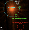 |
Fig. A.1 EPIC/pn image of GJ 643 and GJ 644 AB (ObsID 0860302501). The dashed turquoise circle is centered on the X-ray position of GJ 644 AB and its radius corresponds to the separation of GJ 643 from that bright X-ray source. The three green circles are the background regions chosen for GJ 643, the red circle represents the background region for GJ 644 AB. |
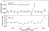 |
Fig. A.2 EPIC/pn background subtracted lightcurve of GJ 643 (black) and the light curve of its background (green), averaged over three regions shown at the top (see Fig. A.1). Lower panel shows, for comparison, the light curve of GJ 644 AB. |
References
- Amard, L., & Matt, S. P. 2020, ApJ, 889, 108 [Google Scholar]
- Ammons, S. M., Robinson, S. E., Strader, J., et al. 2006, ApJ, 638, 1004 [NASA ADS] [CrossRef] [Google Scholar]
- Andrews, J. J., Chanamé, J., & Agüeros, M. A. 2017, MNRAS, 472, 675 [NASA ADS] [CrossRef] [Google Scholar]
- Aschwanden, M. J., & Peter, H. 2017, ApJ, 840, 4 [CrossRef] [Google Scholar]
- Asplund, M., Grevesse, N., Sauval, A. J., & Scott, P. 2009, ARA&A, 47, 481 [NASA ADS] [CrossRef] [Google Scholar]
- Barbera, M., Micela, G., Sciortino, S., Harnden, F. R. J., & Rosner, R. 1993, ApJ, 414, 846 [CrossRef] [Google Scholar]
- Birky, J., Hogg, D. W., Mann, A. W., & Burgasser, A. 2020, ApJ, 892, 31 [Google Scholar]
- Boller, T., Freyberg, M. J., Trümper, J., et al. 2016, A&A, 588, A103 [NASA ADS] [CrossRef] [EDP Sciences] [Google Scholar]
- Briel, U. G., & Pfeffermann, E. 1986, Nucl. Instrum. Methods Phys. Res. A, 242, 376 [CrossRef] [Google Scholar]
- Browning, M. K., Basri, G., Marcy, G. W., West, A. A., & Zhang, J. 2010, AJ, 139, 504 [NASA ADS] [CrossRef] [Google Scholar]
- Butler, R. P., Vogt, S. S., Laughlin, G., et al. 2017, AJ, 153, 208 [Google Scholar]
- Chabrier, G. 2001, ApJ, 554, 1274 [NASA ADS] [CrossRef] [Google Scholar]
- Chadney, J. M., Galand, M., Unruh, Y. C., Koskinen, T. T., & Sanz-Forcada, J. 2015, Icarus, 250, 357 [Google Scholar]
- Cranmer, S. R. 2009, Living Rev. Solar Phys., 6, 3 [NASA ADS] [CrossRef] [Google Scholar]
- Delfosse, X., Forveille, T., Perrier, C., & Mayor, M. 1998, A&A, 331, 581 [NASA ADS] [Google Scholar]
- Díez Alonso, E., Caballero, J. A., Montes, D., et al. 2019, A&A, 621, A126 [NASA ADS] [CrossRef] [EDP Sciences] [Google Scholar]
- Dressing, C. D., & Charbonneau, D. 2013, ApJ, 767, 95 [Google Scholar]
- Favata, F., Reale, F., Micela, G., et al. 2000, A&A, 353, 987 [NASA ADS] [Google Scholar]
- Fleming, T. A. 1998, ApJ, 504, 461 [NASA ADS] [CrossRef] [Google Scholar]
- Fleming, T. A., Schmitt, J. H. M. M., & Giampapa, M. S. 1995, ApJ, 450, 401 [NASA ADS] [CrossRef] [Google Scholar]
- Gaidos, E., Mann, A. W., Lépine, S., et al. 2014, MNRAS, 443, 2561 [Google Scholar]
- Gáspár, A., Rieke, G. H., & Ballering, N. 2016, ApJ, 826, 171 [Google Scholar]
- Gizis, J. E., Reid, I. N., & Hawley, S. L. 2002, AJ, 123, 3356 [Google Scholar]
- Houdebine, E. R. 2012, MNRAS, 421, 3189 [NASA ADS] [CrossRef] [Google Scholar]
- Howard, A. W., Marcy, G. W., Bryson, S. T., et al. 2012, ApJS, 201, 15 [Google Scholar]
- Isaacson, H., Siemion, A. P. V., Marcy, G. W., et al. 2017, PASP, 129, 054501 [NASA ADS] [CrossRef] [Google Scholar]
- Jeffers, S. V., Schöfer, P., Lamert, A., et al. 2018, A&A, 614, A76 [NASA ADS] [CrossRef] [EDP Sciences] [Google Scholar]
- Johnstone, C. P., & Güdel, M. 2015, A&A, 578, A129 [NASA ADS] [CrossRef] [EDP Sciences] [Google Scholar]
- Kirkpatrick, J. D., Marocco, F., Caselden, D., et al. 2021, ApJ, 915, L6 [NASA ADS] [CrossRef] [Google Scholar]
- Lépine, S., & Gaidos, E. 2011, AJ, 142, 138 [Google Scholar]
- Magaudda, E., Stelzer, B., Covey, K. R., et al. 2020, A&A, 638, A20 [NASA ADS] [CrossRef] [EDP Sciences] [Google Scholar]
- Magaudda, E., Stelzer, B., Raetz, S., et al. 2022, A&A, 661, A29 [NASA ADS] [CrossRef] [EDP Sciences] [Google Scholar]
- Maggio, A., Flaccomio, E., Favata, F., et al. 2007, ApJ, 660, 1462 [NASA ADS] [CrossRef] [Google Scholar]
- Maldonado, J., Villaver, E., Eiroa, C., & Micela, G. 2019, A&A, 624, A94 [NASA ADS] [CrossRef] [EDP Sciences] [Google Scholar]
- Mann, A. W., Feiden, G. A., Gaidos, E., Boyajian, T., & von Braun, K. 2015, ApJ, 804, 64 [Google Scholar]
- Mann, A. W., Dupuy, T., Kraus, A. L., et al. 2019, ApJ, 871, 63 [Google Scholar]
- Marfil, E., Tabernero, H. M., Montes, D., et al. 2021, A&A, 656, A162 [NASA ADS] [CrossRef] [EDP Sciences] [Google Scholar]
- Marino, A., Micela, G., & Peres, G. 2000, A&A, 353, 177 [NASA ADS] [Google Scholar]
- Medina, A. A., Winters, J. G., Irwin, J. M., & Charbonneau, D. 2020, ApJ, 905, 107 [Google Scholar]
- Neuhaeuser, R., Sterzik, M. F., Schmitt, J. H. M. M., Wichmann, R., & Krautter, J. 1995, A&A, 297, 391 [NASA ADS] [Google Scholar]
- Neves, V., Bonfils, X., Santos, N. C., et al. 2013, A&A, 551, A36 [NASA ADS] [CrossRef] [EDP Sciences] [Google Scholar]
- Newton, E. R., Charbonneau, D., Irwin, J., et al. 2014, AJ, 147, 20 [Google Scholar]
- Newton, E. R., Irwin, J., Charbonneau, D., et al. 2016, ApJ, 821, 93 [Google Scholar]
- Newton, E. R., Irwin, J., Charbonneau, D., et al. 2017, ApJ, 834, 85 [Google Scholar]
- Orlando, S., Khan, J., van Driel-Gesztelyi, L., et al. 2000a, Adv. Space Res., 25, 1913 [NASA ADS] [CrossRef] [Google Scholar]
- Orlando, S., Peres, G., & Reale, F. 2000b, ApJ, 528, 524 [NASA ADS] [CrossRef] [Google Scholar]
- Orlando, S., Peres, G., & Reale, F. 2001, ApJ, 560, 499 [NASA ADS] [CrossRef] [Google Scholar]
- Orlando, S., Peres, G., & Reale, F. 2004, A&A, 424, 677 [NASA ADS] [CrossRef] [EDP Sciences] [Google Scholar]
- Pallavicini, R., Golub, L., Rosner, R., et al. 1981, ApJ, 248, 279 [NASA ADS] [CrossRef] [Google Scholar]
- Pancino, E., Sanna, N., Altavilla, G., et al. 2021, MNRAS, 503, 3660 [Google Scholar]
- Parker, E. N. 1955, ApJ, 122, 293 [Google Scholar]
- Parker, E. N. 1975, ApJ, 198, 205 [NASA ADS] [CrossRef] [Google Scholar]
- Pecaut, M. J., & Mamajek, E. E. 2013, ApJS, 208, 9 [Google Scholar]
- Peres, G., Orlando, S., Reale, F., Rosner, R., & Hudson, H. 2000, ApJ, 528, 537 [NASA ADS] [CrossRef] [Google Scholar]
- Pinamonti, M., Sozzetti, A., Maldonado, J., et al. 2022, A&A, 664, A65 [NASA ADS] [CrossRef] [EDP Sciences] [Google Scholar]
- Pourbaix, D., Tokovinin, A. A., Batten, A. H., et al. 2004, A&A, 424, 727 [NASA ADS] [CrossRef] [EDP Sciences] [Google Scholar]
- Predehl, P., Andritschke, R., Arefiev, V., et al. 2021, A&A, 647, A1 [EDP Sciences] [Google Scholar]
- Reale, F., Peres, G., & Orlando, S. 2001, ApJ, 557, 906 [CrossRef] [Google Scholar]
- Reiners, A., Joshi, N., & Goldman, B. 2012, AJ, 143, 93 [Google Scholar]
- Reylé, C., Jardine, K., Fouqué, P., et al. 2021, A&A, 650, A201 [Google Scholar]
- Riello, M., De Angeli, F., Evans, D. W., et al. 2021, A&A, 649, A3 [NASA ADS] [CrossRef] [EDP Sciences] [Google Scholar]
- Robrade, J., & Schmitt, J. H. M. M. 2005, A&A, 435, 1073 [NASA ADS] [CrossRef] [EDP Sciences] [Google Scholar]
- Rojas-Ayala, B., Covey, K. R., Muirhead, P. S., & Lloyd, J. P. 2012, ApJ, 748, 93 [Google Scholar]
- Rosat, C. 2000, VizieR Online Data Catalog: IX/30 [Google Scholar]
- Saar, S. H., & Testa, P. 2012, IAU Symp., 286, 335 [Google Scholar]
- Sanz-Forcada, J., Micela, G., Ribas, I., et al. 2011, A&A, 532, A6 [NASA ADS] [CrossRef] [EDP Sciences] [Google Scholar]
- Schmitt, J. H. M. M. 1997, A&A, 318, 215 [NASA ADS] [Google Scholar]
- Schmitt, J. H. M. M. 2012, IAU Symp., 286, 296 [NASA ADS] [Google Scholar]
- Schmitt, J. H. M. M., & Liefke, C. 2004, A&A, 417, 651 [NASA ADS] [CrossRef] [EDP Sciences] [Google Scholar]
- Schmitt, J. H. M. M., Fleming, T. A., & Giampapa, M. S. 1995, ApJ, 450, 392 [Google Scholar]
- Schöfer, P., Jeffers, S. V., Reiners, A., et al. 2019, A&A, 623, A44 [Google Scholar]
- Soubiran, C., Jasniewicz, G., Chemin, L., et al. 2018, A&A, 616, A7 [NASA ADS] [CrossRef] [EDP Sciences] [Google Scholar]
- Stelzer, B., Marino, A., Micela, G., López-Santiago, J., & Liefke, C. 2013, MNRAS, 431, 2063 [Google Scholar]
- Stelzer, B., Bogner, M., Magaudda, E., & Raetz, S. 2022a, A&A, 665, A30 [NASA ADS] [CrossRef] [EDP Sciences] [Google Scholar]
- Stelzer, B., Caramazza, M., Raetz, S., Argiroffi, C., & Coffaro, M. 2022b, A&A, 667, A9 [NASA ADS] [CrossRef] [EDP Sciences] [Google Scholar]
- van den Besselaar, E. J. M., Raassen, A. J. J., Mewe, R., et al. 2003, A&A, 411, 587 [NASA ADS] [CrossRef] [EDP Sciences] [Google Scholar]
- Voges, W., Aschenbach, B., Boller, T., et al. 1999, A&A, 349, 389 [NASA ADS] [Google Scholar]
- Voges, W., Aschenbach, B., Boller, T., et al. 2000, IAU Circ., 7432, 3 [NASA ADS] [Google Scholar]
- Webb, N. A., Coriat, M., Traulsen, I., et al. 2020, A&A, 641, A136 [NASA ADS] [CrossRef] [EDP Sciences] [Google Scholar]
- Wenger, M., Ochsenbein, F., Egret, D., et al. 2000, A&AS, 143, 9 [NASA ADS] [CrossRef] [EDP Sciences] [Google Scholar]
- West, A. A., Weisenburger, K. L., Irwin, J., et al. 2015, ApJ, 812, 3 [NASA ADS] [CrossRef] [Google Scholar]
- White, S. M., Kundu, M. R., Garaimov, V. I., Yokoyama, T., & Sato, J. 2002, ApJ, 576, 505 [CrossRef] [Google Scholar]
- Zechmeister, M., & Kürster, M. 2009, A&A, 496, 577 [CrossRef] [EDP Sciences] [Google Scholar]
- Zhang, L.-Y., Meng, G., Long, L., et al. 2021, ApJS, 253, 19 [NASA ADS] [CrossRef] [Google Scholar]
All Tables
Conversion factor between count rate measured with different X-ray instruments and flux in the 0.1–2.4 keV ROSAT band.
Upper limit count rates and effective exposure time after removal high-background time intervals for GJ 745 A during the two XMM-Newton observations.
X-ray surface fluxes for magnetic structures (BKC, AR, and CO) in the corona of the Sun obtained from Yohkoh data collected in July 1996 (during a minimum in the solar cycle) within the Sun as an X-ray star framework.
All Figures
|
Fig. 1 Gaia color–magnitude diagram for the 10 pc census from Reylé et al. (2021). The stars with unreliable GBP magnitudes are shown in gray and the selected M10PC-Gaia SAMPLE (restricted to SpT M0…M4) is highlighted in red. Superposed is the main-sequence from E. Mamajek’s table (see https://www.pas.rochester.edu/~emamajek/EEM_dwarf_UBVIJHK_colors_Teff.txt). |
| In the text | |
|
Fig. 2 X-ray luminosity versus distance for the M 10PC-GAIA SAMPLE. For stars detected more than once, the Lx value from the deepest survey was used in the order explained in the text. Among all the other stars, only one has remained undetected, namely, GJ 745 A, which has an upper limit indicated by the downward pointing arrow. |
| In the text | |
|
Fig. 3 X-ray surface flux versus Gaia GBP – GRP color for the M 10PC-GAIA SAMPLE. Each star is represented by its mean X-ray emission level from our multi-mission data base. Colored areas mark the range of surface flux for four typical non-flaring magnetic regions in the solar corona, coronal holes (CH), background corona (BKC), active regions (AR), and cores of active regions (CO); see Table 3. The flux ranges of the BKC and CH overlap. Only two stars are located within or in the immediate vicinity of the “coronal hole” area: the binary pair GJ 745 A and B, where the upper limit is given for the A component of the system. |
| In the text | |
|
Fig. 4 Hardness ratios of the stars from the M 10PC-GAIA SAMPLE that are detected with XMM-Newton (filled black squares), with the CH star (in blue) highlighted. Superposed on the data is a grid of 2T-APEC models with a fixed kT1 at 0.1 keV, kT2 and EM2/EM1 ranging from 0.1 keV to 0.9 keV and 0.2 to 12, respectively (see Sect. 4.2.1 for more details). |
| In the text | |
|
Fig. 5 Background-subtracted EPIC/pn light curve of GJ 745 B (black) and light curve of the background (green), both with a bin size of 800 s (see Sect. 4.2.1). We also show the quiescent rate with its standard deviation (red dashed line and shade, respectively) that we adopted for the calculation of the flare energy as explained in Sect. 4.2.2. The light curve is shorter than the nominal exposure time due to high and variable background at the end of the observation. |
| In the text | |
|
Fig. 6 Metallicity of the M 10PC-GAIA SAMPLE extracted from the literature cited in Sect. 4.2.3. The coronal hole stars are highlighted. |
| In the text | |
|
Fig. A.1 EPIC/pn image of GJ 643 and GJ 644 AB (ObsID 0860302501). The dashed turquoise circle is centered on the X-ray position of GJ 644 AB and its radius corresponds to the separation of GJ 643 from that bright X-ray source. The three green circles are the background regions chosen for GJ 643, the red circle represents the background region for GJ 644 AB. |
| In the text | |
|
Fig. A.2 EPIC/pn background subtracted lightcurve of GJ 643 (black) and the light curve of its background (green), averaged over three regions shown at the top (see Fig. A.1). Lower panel shows, for comparison, the light curve of GJ 644 AB. |
| In the text | |
Current usage metrics show cumulative count of Article Views (full-text article views including HTML views, PDF and ePub downloads, according to the available data) and Abstracts Views on Vision4Press platform.
Data correspond to usage on the plateform after 2015. The current usage metrics is available 48-96 hours after online publication and is updated daily on week days.
Initial download of the metrics may take a while.