| Issue |
A&A
Volume 676, August 2023
|
|
|---|---|---|
| Article Number | A100 | |
| Number of page(s) | 18 | |
| Section | Cosmology (including clusters of galaxies) | |
| DOI | https://doi.org/10.1051/0004-6361/202346025 | |
| Published online | 17 August 2023 | |
Aether scalar tensor theory confronted with weak lensing data at small accelerations
1
Frankfurt Institute for Advanced Studies, Ruth-Moufang-Str. 1, 60438 Frankfurt am Main, Germany
e-mail: This email address is being protected from spambots. You need JavaScript enabled to view it.
2
Department of Astronomy, Case Western Reserve University, 10900 Euclid Avenue, Cleveland, OH 44106, USA
3
Munich Center for Mathematical Philosophy, Ludwig-Maximilians-Universität, Geschwister-Scholl-Platz 1, 80539 München, Germany
Received:
30
January
2023
Accepted:
28
June
2023
Abstract
Context. The recently proposed aether scalar tensor (AeST) model reproduces both the successes of particle dark matter on cosmological scales and those of modified Newtonian dynamics (MOND) on galactic scales. But the AeST model reproduces MOND only up to a certain maximum galactocentric radius. Since MOND is known to fit very well to observations at these scales, this raises the question of whether the AeST model comes into tension with data.
Aims. We tested whether or not the AeST model is in conflict with observations using a recent analysis of data for weak gravitational lensing.
Methods. We solved the equations of motion of the AeST model, analyzed the solutions’ behavior, and compared the results to observational data.
Results. The AeST model shows some deviations from MOND at the radii probed by weak gravitational lensing. The data show no clear indication of these predicted deviations.
Key words: galaxies: kinematics and dynamics / gravitational lensing: weak / dark matter / gravitation
© The Authors 2023
 Open Access article, published by EDP Sciences, under the terms of the Creative Commons Attribution License (https://creativecommons.org/licenses/by/4.0), which permits unrestricted use, distribution, and reproduction in any medium, provided the original work is properly cited.
This article is published in open access under the Subscribe to Open model. This email address is being protected from spambots. You need JavaScript enabled to view it. to support open access publication.
1. Introduction
Recently, various models have been proposed that combine the successes of modified Newtonian dynamics (MOND, Milgrom 1983a,b,c; Bekenstein & Milgrom 1984) on galactic scales with those of the Λ cold dark matter model (ΛCDM) on cosmological scales. Examples are superfluid dark matter (SFDM, Berezhiani & Khoury 2015; Berezhiani et al. 2018), the aether scalar tensor (AeST) model (Skordis & Złosnik 2021, 2022), and the neutrino-based model by Angus (2009; νHDM). The focus of the present paper is on the AeST model. An accompanying paper will look at SFDM.
The AeST model is a relativistic model that can reproduce MOND in the vicinity of galaxies and fits the fluctuations in the cosmic microwave background (CMB) as well as the matter power spectrum. In addition, it has a tensor mode that propagates at the speed of light which avoids difficulties matching the observations associated with GW170817 (Sanders 2018; Boran et al. 2018).
An important ingredient in the AeST model is a so-called ghost condensate (Arkani-Hamed et al. 2004, 2007). This ghost condensate is the major difference between the action of the AeST model in the static limit and the standard MOND-type action for multifield theories (Famaey & McGaugh 2012). The ghost condensate has an energy density that acts as an additional source for the gravitational field equations.
The integrated mass of the ghost condensate is generally negligible close to galaxies, where rotation curves are measured. Beyond a few hundred kiloparsecs, however, the ghost condensate mass is no longer negligible compared to the baryonic mass which leads to deviations from MOND.
This is a desired feature for galaxy clusters where observations require accelerations larger than what MOND predicts (Aguirre et al. 2001; Sanders 2003; Eckert et al. 2022). It may, however, be in conflict with unprecedented recent observations at large radii around galaxies: The analysis of weak-gravitational lensing data from Brouwer et al. (2021) found MOND-like behavior around galaxies up to ∼1 Mpc. Here, we explore whether this finding is compatible with the AeST model.
Since MOND is known to fit these observations well, we adopt an indirect approach to comparing the AeST model to observations. First, we introduce a method to quantify the deviation of the AeST model from MOND and analyze for which solutions these deviations are minimal. We then compare these optimal solutions – as well as slightly suboptimal ones – to the observational data.
2. Equations of motion and chemical potential
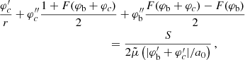
For galaxies we can use the quasi-static weak-field limit of the AeST model. In this limit, the model can be described by two fields,  and φ, whose equations of motion are (at least in the spherically symmetric case that interests us here, see Appendix A),
 (1a)
(1a)
 (1b)
(1b)
where a0 is the MOND acceleration scale and fG is the conversion factor between Newton’s gravitational constant GN and the constant  that appears in the Lagrangian (see Appendix A). We use a0 = 1.2 × 10⁻¹⁰ m s−2 (Lelli et al. 2017). Both fields are sourced by the baryonic energy density ρb and the ghost condensate density ρc. The function
  can be freely chosen in this model and corresponds to an interpolation function of MOND. That is, it determines how the model interpolates between Newtonian gravity at large accelerations and MOND-like gravity at small accelerations. The constant fG determines how much of the total acceleration (see below) in the Newtonian limit is due to φ and how much is due to
  .
.
In the AeST model, ordinary matter couples to the metric gμν in the usual way. The metric has the same form as in general relativity (GR), but with the Newtonian potential Φ being a combination of  and φ, namely
  . Thus, the total acceleration felt by matter is
  .
.
The ghost condensate energy density ρc is given by
 (2)
(2)
where m and Q0 are constants. For cosmology, Skordis & Złosnik (2021) considered nonlinear corrections to this. We do not include these here for reasons discussed in Appendix I.
We did not set  in Eq. (2) because any constant
  still gives time-independent equations of motion. Indeed,
  represents the chemical potential of the condensate. To see this, one first observes that the model is shift-symmetric under
  ,
,  for any constant
  . In general, to describe equilibrium states, one introduces a chemical potential μ for each symmetry by shifting the Hamiltonian H by H → H − μ Q where Q is the conserved quantity associated with the symmetry. In the AeST model and on the level of the Lagrangian, this corresponds to shifting
  and
and  (Mistele 2019; Kapusta 1981; Haber & Weldon 1982; Bilic 2008) or equivalently to considering solutions with
  and
and  . (We note that the parameter m was called μ in Skordis & Złosnik 2021. We use μ instead to denote the chemical potential).
Consequently, the behavior of the AeST model around galaxies depends on the choice of this chemical potential of the ghost condensate. This corresponds to a choice of boundary condition for the combination μ/Q0 − Φ which is a gauge-invariant variable as shown in Skordis & Złosnik (2022). This is an important difference to MOND where ρb alone determines the phenomenology around galaxies.
For real galaxies, these chemical potentials are ultimately set by galaxy formation. Since no simulations of nonlinear structure formation in the AeST model are available, we treated the chemical potential of each galaxy as a free parameter. In this regard, the AeST model is similar to SFDM. Both models require a choice of chemical potential to make predictions in galaxies (Berezhiani & Khoury 2015; Berezhiani et al. 2018; Mistele 2019, 2021; Hossenfelder & Mistele 2020; Mistele et al. 2022).
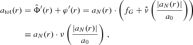
We now assume spherical symmetry. Then, solutions have the same form as in MOND, just with the baryonic mass replaced by an effective mass that includes the condensate mass,
 (3)
(3)
Thus, with the Newtonian acceleration aN in the negative radial direction,
 (4)
(4)
we can write the total acceleration in the negative radial direction atot as atot = aN(r)⋅ν(|aN(r)|/a0) where the interpolation function ν is determined by the free function  in the AeST model (see Eq. (1)). Unlike in MOND, aN can be negative because the condensate mass Mc can be negative. We discuss this in more detail below.
For simplicity, we chose the interpolation function such that
 (5)
(5)
where seff is the sign of Meff. We recover MOND by leaving out the contributions from the condensate, Mc = 0. Thus, when comparing the AeST model to MOND below, we assumed the following acceleration for MOND,
 (6)
(6)
This assumes the same interpolation function for MOND and the AeST model.
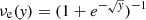
This interpolation function has the correct limits, namely aMOND → ab for accelerations much larger than a0 and  for accelerations much smaller than a0. Still, in general, this choice is too simplistic. But it suffices for our purposes because we are only interested in the small-acceleration regime where all interpolation functions give
 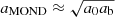 .
.
The total acceleration atot in the AeST model does not explicitly depend on fG and is the sum of  and
and  . Below, we refer to its MOND-like part
  and its Newton-like part aN, respectively, as
 (7)
(7)
In the following we assumed point particle baryonic masses for simplicity. This suffices for our purposes, because the details of the baryonic mass distribution do not matter much at the large galactocentric radii we consider. See Appendix D for an approximate analytical solution for this case and Appendix E for how we calculate numerical solutions.
3. Deviations from MOND
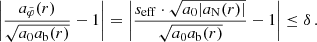
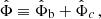
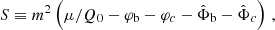
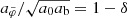
The AeST model reproduces MOND so long as the condensate’s total mass is small compared to the baryonic mass. This condition is usually fulfilled in the inner parts of galaxies but not far away from the galaxy. Indeed, given a maximum allowed fractional deviation δ from MOND, there is an optimal boundary condition for which the MOND-like behavior extends to a finite maximum radius rmax. For all other boundary conditions, deviations from MOND set in earlier. This is illustrated in Fig. 1.
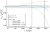 |
Fig. 1. Numerical solution with the optimal boundary condition for δ = 0.05 (solid blue line). That is, the solution for which |


Specifically, we imposed the maximum allowed deviation δ as
 (8)
(8)
That is, we compared the accelerations in the AeST model and MOND, focusing on the MOND-like contributions  and
and  . Alternatively, one could compare the total acceleration in both models, that is,
  and
and  . But at the large radii we consider here, the difference is negligible (see Appendix G) and we used Eq. (8) for simplicity.
The maximal radius rmax, up to which we allowed accelerations to deviate by less than a fraction δ from MOND, is given by
 (9)
(9)
Here, rMOND is a constant known as the MOND-radius  . See Appendix G for a derivation of those properties and an analysis of the conditions under which this estimate holds.
This maximum radius rmax scales as  . This means that more massive galaxies can stay close to MOND up to larger radii than less massive galaxies. In MOND, however, accelerations ab = GNMb/r2 are more relevant than radii r. For example, the Radial Acceleration Relation (RAR, Lelli et al. 2017) relates the total acceleration atot and the Newtonian baryonic acceleration ab.
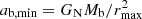
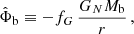
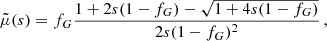
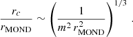
The maximum radius rmax corresponds to a minimum acceleration  which scales as
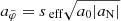
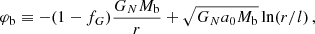
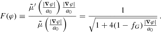
  . Thus, in acceleration space, less massive galaxies can stay close to MOND for longer than more massive galaxies. We show ab, min in Fig. 2 and illustrate the RAR for various baryonic masses in Fig. 3.
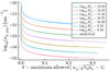 |
Fig. 2. Acceleration |

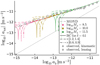 |
Fig. 3. RAR for different baryonic masses and boundary conditions for numerical solutions with fG/m2 = 0.99 Mpc2. The solid lines are for boundary conditions where |

The scale of rmax is set by the combination m2/fG. Skordis & Złosnik (2021) require m2/fG ≲ 1 Mpc−2. As we show below, this does not guarantee MOND-like behavior for weak lensing which probes radii up to ∼1 Mpc. One might therefore want to choose an even smaller m2/fG. But this is not easily possible. Indeed, galaxy clusters require more acceleration than MOND predicts (Aguirre et al. 2001; Sanders 2003; Eckert et al. 2022). To naturally explain this in the AeST model, m2/fG cannot be much smaller than 1 Mpc−2 and we assumed
 (10)
(10)
We obtained this estimate by requiring that the minimum acceleration ab, min in AeST matches where observed clusters deviate from MOND. For example, if we require that the total acceleration atot in a cluster with Mb = 1014 M⊙ deviates by at least δ = 10% from MOND at ab, min = 10−10.5 m s−2, we find m2/fG > 2.5 Mpc−2 (see also Table 1)1.
Rough bounds on m2/fG.
Beyond the radius where the AeST model deviates from MOND, the gravitational force eventually becomes oscillatory (Skordis & Złosnik 2021), see also Appendix F, as is typical for condensate models (Arkani-Hamed et al. 2007). The reason is that Meff(r) and the condensate density ρc oscillate. However, condensates with negative energy-density are unstable (or at least we would expect a good reason for why they are not unstable). We therefore expect the AeST model to be unstable in this oscillatory regime. We would then no longer have a macroscopically coherent condensate and the quasi-static action Eq. (A.1) is no longer good to use.
In superfluid dark matter models, for example, we assume that when the energy-density begins to oscillate that we have to continue the condensate density by a standard (nonsuperfluid) phase (Berezhiani & Khoury 2015; Berezhiani et al. 2018). Something similar might happen in the AeST model.
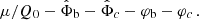
However, so far, a stability analysis for the AeST model in a galactic background has not been done, so maybe the oscillatory regime turns out to be stable after all. Below, we therefore keep in mind both possibilities and discuss where our results depend on whether or not negative condensate densities are stable. For example, Fig. 4 shows the solutions from Fig. 3 but truncated where the condensate density first drops to zero.
 |
Fig. 4. Same as Fig. 3 but with all solutions truncated where the condensate density first drops to zero, that is, truncated where the solutions become potentially unstable. |
4. Weak lensing
The AeST model usually reproduces MOND at the radii probed by rotation curves because the condensate density Mc is negligible there. This means that probing the effects of the condensate requires a different approach. The option we pursued here is to use the recent weak-lensing analysis of Brouwer et al. (2021) who find that accelerations are MOND-like down to at least ab ∼ 10−13 m s−2.
In the AeST model, matter is coupled to the fields φ and  through the metric gμν. In the weak-field limit, this metric has the same form as in GR, just with the Newtonian potential replaced by
  . We can therefore use the standard formalism for weak lensing just by taking into account
  .
.
Most galaxies in the weak-lensing sample from Brouwer et al. (2021) have baryonic masses between 1010 M⊙ and 1011 M⊙. For the AeST model with fG/m2 = 0.99 Mpc2, Fig. 2 shows that MOND-like behavior up to a few 10% is possible down to ab ∼ 10−13 m s−2 for those galaxies in the sample with baryonic masses ∼1010 M⊙.
Such 𝒪(10%) deviations may be sufficient to match observations. But it is important to keep in mind that in this regime where deviations from MOND start to become important, the details depend on the precise baryonic masses and boundary conditions of the galaxy sample as well as the precise value of the model parameter m2/fG. For example, Fig. 2 shows solutions for boundary conditions that are optimal for reproducing MOND. But there is no reason why galaxy formation should result in such optimal boundary conditions. One would therefore expect deviations of AeST from MOND to generally be larger than in the optimal case we depict.
We can derive a rough upper bound on the model parameter m2/fG by requiring that AeST can reproduce MOND in the regime probed by weak lensing. For this, we used the minimum acceleration  with rmax from Eq. (9). Many of the galaxies in the sample used by Brouwer et al. (2021) have baryonic masses close to 1011 M⊙. If we require that such galaxies can reproduce MOND down to ab, min = 10−15 m s−2 and up to a fraction δ = 10%, we find m2/fG < 0.001 Mpc−2. There is a lot of uncertainty in this upper bound. For example, m2/fG = 0.001 Mpc−2 is small enough that the ghost condensate density in galaxies as given by Eq. (2) is typically smaller than the cosmological background density. So, at least in principle, there could be corrections from the fact that we should expand around a cosmological background, not around empty Minkowski space (which is how Eq. (1) was derived)2. Also, if we disregard the data below ab = 10−13 m s−2 because the isolation criterion used in the weak-lensing analysis is less reliable there (Brouwer et al. 2021), we obtain the weaker bound m2/fG < 1 Mpc−2. Still, a tension between the value of m2/fG required by weak lensing and that required by galaxy clusters, m2/fG ≳ 1 Mpc−2, seems likely (see Table 1).
Another aspect to take into account is that, in practice, the weak-lensing RAR is not known for individual galaxies. It is known only in an averaged sense for a large sample of stacked galaxies. It is possible that stacking gives a MOND-like RAR even if most galaxies individually do not. As we show in Appendix H, in our case, stacking simply means calculating a weighted average in acceleration space. So, indeed, accelerations larger than MOND from some galaxies can cancel accelerations smaller than MOND from other galaxies.
To illustrate this, we considered a sample of galaxies with a fixed baryonic mass Mb but various boundary conditions. For simplicity, we weighed all galaxies equally when averaging. One example is shown in Fig. 5. We see how a stacked RAR can be MOND-like even when most individual stacked galaxies are not. Of course, one does not always get a MOND-like RAR from stacking. This works only when accelerations below and above the MOND prediction cancel each other. Whether or not it works for real lensing galaxies depends on which boundary conditions are picked by galaxy formation.
 |
Fig. 5. RAR for solutions with fixed baryonic mass Mb = 1011 M⊙ for various boundary conditions (green dotted lines) and the corresponding stacked RAR (solid red line). This is for fG/m2 = 0.99 Mpc2. The boundary conditions of the individual solutions are in the range 0.5 − 1.5 times the optimal boundary condition for δ = 0.05 with a step size of 0.1 times the optimal one. Solutions are cut off where the first of the individual solutions reaches atot = 0. We also show the analytically stacked RAR according to formula Eq. (H.9). |
In addition, stacking galaxies with different boundary conditions should lead to increased uncertainties at small ab where different boundary conditions lead to significantly different accelerations. In principle, such uncertainties might be visible in the error bars of the observed weak-lensing RAR.
However, we expect that in practice there is often no visible effect on the error bars. To see this, we first note that the error bars shown in Figs. 3 and 4 correspond to the uncertainty of the mean value of atot, obtained by stacking a large number N of galaxies. They do not represent the scatter from galaxy-by-galaxy variation. The galaxy-by-galaxy variation is larger than the uncertainty of the mean by a factor of about  . In AeST, different boundary conditions induce a form of galaxy-by-galaxy variation. Thus, the scatter from solutions with different boundary conditions should be compared to the larger galaxy-by-galaxy variation and not to the uncertainty of the mean. Put differently, the scatter induced by different boundary conditions should be scaled by a factor
  before comparing to the error bars shown in Figs. 3 and 4. Here, N is on the order of 105 (Brouwer et al. 2021). Thus, one would expect a visible effect on the error bars only in extreme cases.
4.1. Negative condensate densities
Whether or not stacked galaxies can follow a MOND RAR down to smaller accelerations than individual galaxies also depends on whether or not negative condensate densities are stable. To see this, we note that accelerations are smaller than in MOND if and only if the effective mass Meff = Mb + Mc is smaller than in MOND. This is only possible for negative Mc which requires negative condensate densities. Therefore, if negative densities are unstable, cancelling accelerations that are larger against those that are smaller than in MOND does not work. This is simply because all accelerations are larger than in MOND if we do not allow for negative densities. This is illustrated in Fig. 6.
 |
Fig. 6. Same as Fig. 5 but with all individual stacked solutions having positive condensate density. The individual solutions are for boundary conditions in the range 1.0 − 2.0 times the optimal boundary condition for δ = 0.05 with a step size of 0.1 times the optimal one. Solutions are cut off where the first of the individual solutions reaches ρc = 0. |
Thus, if negative densities are unstable, one might expect that the AeST model always gives larger accelerations than MOND. Moreover, our estimate for ab, min (see Fig. 2) suggests that these deviations should set in earlier for larger baryonic masses Mb. And indeed, there are hints of such behavior in the observed weak-lensing data, see Fig. 7 which shows the weak-lensing data separately for early-type galaxies (ETGs) and late-type galaxies (LTGs). We see that the weak-lensing RAR for LTGs follows the MOND prediction even for ab < 10−13 m s−2 while ETGs tend toward larger accelerations than MOND. In general, ETGs have larger baryonic masses than LTGs. So this seems to fit with the AeST model expectations if negative densities are unstable.
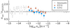 |
Fig. 7. Observed weak-lensing RAR for ETGs and LTGs from Brouwer et al. (2021) with the stellar M/L* corrected to use the same stellar population model as the observed kinematic RAR (McGaugh 2022, priv. comm.) relative to the MOND prediction. This does not include the hot gas estimate from Brouwer et al. (2021). Here, we take aMOND = abνe(ab/a0) with |
However, this Mb-dependence is not a plausible explanation for the difference between the observed weak-lensing RARs for ETGs and LTGs. This is for three reasons.
First, the ETGs and LTGs do not sufficiently differ in baryonic mass. What would be required is a difference in Mb of more than a factor 103/2. To see this, we note that LTGs follow the MOND prediction for at least one more order of magnitude in ab compared to ETGs. This translates into a factor > 103/2 in terms of baryonic mass according to our estimate  . In contrast, Brouwer et al. (2021) selected LTGs and ETGs to have the same stellar mass distribution. With the stellar M/L scale corrected to be consistent with that of the observed kinematic RAR, ETG stellar masses would still be larger by a factor 1.4 (McGaugh, priv. comm.). But this is not sufficient here.
Of course, the total baryonic mass should take into account gas, but this is unlikely to account for the required factor of 103/2 or more, at least with the simple cold gas mass estimate used in Brouwer et al. (2021). Brouwer et al. (2021) also consider a scenario where ETGs have significantly more hot gas than LTGs. But even in that scenario, the baryonic masses of ETGs differ from those of LTGs by only a factor of two or a bit more. In addition, adopting this scenario means adopting a different observed lensing RAR. Indeed, as discussed in Brouwer et al. (2021), in this scenario there might not even be a discrepancy between ETGs and LTGs left to explain.
Second, the isolation criterion needed to obtain the weak-lensing RAR might fail for ETGs sooner than it does for LTGs. One might naturally expect this to be the case since ETGs are known to be more clustered than LTGs (Dressler 1980). At what point this comes into play here we cannot judge, but mention it as a logical possibility.
Third and finally, even if negative densities are indeed unstable, the AeST model does not necessarily predict larger accelerations than MOND. Indeed, it makes no physical sense to stop looking when the condensate becomes unstable. In a real galaxy, something else must follow after the condensate phase. For example, the macroscopically coherent ghost condensate might be replaced by something closer to a ΛCDM-like collisionless fluid which the AeST model postulates on cosmological scales (Skordis & Złosnik 2021). In principle, whatever replaces the ghost condensate might lead to smaller accelerations than MOND.
That said, the prediction of larger-than-MOND accelerations remains valid if whatever replaces the ghost condensate has as its only effect to replace the ghost condensate density by some other positive density, ρc → ρreplace. This is because then one still has solutions of the same form as before, just with a different effective mass Meff → Mb + Mreplace > Mb.
In order to get smaller-than-MOND accelerations, the general structure of the solutions must be modified. That is, the left-hand sides of the equations of motions must be modified,  . It is not implausible that this indeed happens since the field φ plays a role for both the ghost condensate (for example, it carries the chemical potential
  ) as well as the gravitational force. So outside the condensate phase both could be modified.
4.2. External field effect
Another concern at the small accelerations probed by weak lensing is the external field effect (EFE) of MOND (Milgrom 1983b; Famaey & McGaugh 2012). The EFE is a consequence of the specific nonlinear form ∇(|∇φ|∇φ)∝ρb of the gravitational field equations in the small-acceleration limit. The crucial nonlinearity is the same in the AeST model, so there is probably a similar effect there, at least within the ghost condensate3.
The EFE generally reduces the observationally inferred atot, while a condensate mass Mc > 0 in the AeST model enhances this acceleration. In principle, these two effects could cancel each other to give a MOND-like acceleration even at very large galactocentric distances, but there is no reason to expect such a cancellation to generally happen.
And in any case, if negative densities are unstable and the condensate is replaced by something else at large radii, then any potential EFE depends on the details of what replaces the ghost condensate. There could be a modified nonlinear effect that still allows neighboring galaxies to affect each other in a way that violates the Strong Equivalence Principle (SEP) like the MOND EFE does. Or there could be no such effect, possibly restoring the SEP at large scales.
A restored SEP would fit with the fact that the observed weak-lensing RAR from Brouwer et al. (2021) shows no signs of an EFE. But here one must be careful. The EFE pertains to nonisolated galaxies, while the analysis of Brouwer et al. (2021) requires isolated galaxies. Thus, any EFE effects may be masked by violations of this assumption. In addition, the environment-dependence of the EFE is quite complicated (Llinares et al. 2008; Chae et al. 2021). So it is not even clear for MOND whether or not a significant EFE is expected here. Still, the EFE is something to keep in mind as observations and theoretical predictions are improved.
5. Conclusion
We have explored whether or not the AeST model can explain the observed MOND-like weak-lensing RAR which probes unprecedentedly small accelerations. We find that deviations from MOND start to set in already in the range of the new measurements, creating a tension with data. The model parameter m2/fG can be adjusted to avoid this tension, but that likely creates a tension with observations of galaxy clusters instead.
It seems that keeping the model in agreement with data would require specific values of boundary conditions for a large variety of galaxies. While this is possible, we do not know of any mechanism that would result in these particular boundary conditions. Thus, while we cannot rule out the model, it does seem that weak-lensing observations pose a challenge for AeST.
Here, we did not use the analytical estimate Eq. (9) for rmax when calculating  . The reason is that Eq. (9) is derived using approximations that are better for galaxies than for clusters. Instead, we calculated rmax from numerical solutions of the equations of motion. Using Eq. (9) would give m2/fG > 7.9 Mpc−2.
But we note that there is no reason to expect that such corrections would help to explain why weak-lensing observations follow the MOND prediction down to very small accelerations ab.
The EFE is only relevant in situations that are not spherically symmetric. In these cases, as we discuss in Appendix B, the vector field A of the AeST model cannot be set to zero and the equations of motion are not given by Eq. (1). Still, there is the same type of nonlinearity and it is plausible that an effect similar to the MOND EFE exists.
Of course, in contrast to Skordis & Złosnik (2021), we did not run a full cosmological perturbations calculation. We only considered the constraint on w from the background cosmology. It is possible that new constraints arise from the CMB or other observations pertaining to cosmological perturbation theory. Here, we assume that this is not the case.
Acknowledgments
We thank Margot Brouwer, Andrej Dvornik, and Kyle Oman for helpful correspondence. This work was supported by the DFG (German Research Foundation) under grant number HO 2601/8-1 together with the joint NSF grant PHY-1911909. This work was supported by the DFG (German Research Foundation) – 514562826.
References
- Aguirre, A., Schaye, J., & Quataert, E. 2001, ApJ, 561, 550 [NASA ADS] [CrossRef] [Google Scholar]
- Angus, G. W. 2009, MNRAS, 394, 527 [NASA ADS] [CrossRef] [Google Scholar]
- Arkani-Hamed, N., Cheng, H. S., Luty, M. A., & Mukohyama, S. 2004, J. High Energy Phys., 2004, 074 [CrossRef] [Google Scholar]
- Arkani-Hamed, N., Cheng, H.-C., Luty, M. A., Mukohyama, S., & Wiseman, T. 2007, J. High Energy Phys., 2007, 036 [CrossRef] [Google Scholar]
- Berezhiani, L., & Khoury, J. 2015, Phys. Rev. D, 92, 103510 [Google Scholar]
- Bekenstein, J., & Milgrom, M. 1984, ApJ, 286, 7 [NASA ADS] [CrossRef] [Google Scholar]
- Berezhiani, L., Famaey, B., & Khoury, J. 2018, J. Cosmol. Astropart. Phys., 1809, 021 [CrossRef] [Google Scholar]
- Bilic, N. 2008, Phys. Rev. D, 78, 105012 [NASA ADS] [CrossRef] [Google Scholar]
- Boran, S., Desai, S., Kahya, E. O., & Woodard, R. P. 2018, Phys. Rev. D, 97, 041501 [NASA ADS] [CrossRef] [Google Scholar]
- Brada, R., & Milgrom, M. 1995, MNRAS, 276, 453 [Google Scholar]
- Brouwer, M. M., Oman, K. A., Valentijn, E. A., et al. 2021, A&A, 650, A113 [NASA ADS] [CrossRef] [EDP Sciences] [Google Scholar]
- Chae, K.-H., Desmond, H., Lelli, F., McGaugh, S. S., & Schombert, J. M. 2021, ApJ, 921, 104 [NASA ADS] [CrossRef] [Google Scholar]
- Dressler, A. 1980, ApJ, 236, 351 [Google Scholar]
- Eckert, D., Ettori, S., Pointecouteau, E., van der Burg, R. F. J., & Loubser, S. I. 2022, A&A, 662, A123 [NASA ADS] [CrossRef] [EDP Sciences] [Google Scholar]
- Famaey, B., & McGaugh, S. S. 2012, Liv. Rev. Relat., 15, 10 [Google Scholar]
- Haber, H. E., & Weldon, H. A. 1982, Phys. Rev. D, 25, 502 [NASA ADS] [CrossRef] [Google Scholar]
- Hossenfelder, S., & Mistele, T. 2020, MNRAS, 498, 3484 [NASA ADS] [CrossRef] [Google Scholar]
- Ilić, S., Kopp, M., Skordis, C., & Thomas, D. B. 2021, Phys. Rev. D, 104, 043520 [Google Scholar]
- Kapusta, J. I. 1981, Phys. Rev. D, 24, 426 [NASA ADS] [CrossRef] [Google Scholar]
- Lelli, F., McGaugh, S. S., Schombert, J. M., & Pawlowski, M. S. 2017, ApJ, 836, 152 [Google Scholar]
- Llinares, C., Knebe, A., & Zhao, H. 2008, MNRAS, 391, 1778 [NASA ADS] [CrossRef] [Google Scholar]
- Milgrom, M. 1983a, ApJ, 270, 371 [Google Scholar]
- Milgrom, M. 1983b, ApJ, 270, 365 [Google Scholar]
- Milgrom, M. 1983c, ApJ, 270, 384 [Google Scholar]
- Milgrom, M. 2021, Phys. Rev. D, 103, 044043 [NASA ADS] [CrossRef] [Google Scholar]
- Mistele, T. 2019, J. Cosmol. Astropart. Phys., 1911, 039 [CrossRef] [Google Scholar]
- Mistele, T. 2021, J. Cosmol. Astropart. Phys., 2021, 025 [CrossRef] [Google Scholar]
- Mistele, T., McGaugh, S., & Hossenfelder, S. 2022, A&A, 664, A40 [NASA ADS] [CrossRef] [EDP Sciences] [Google Scholar]
- Mogensen, P. K., & Riseth, A. N. 2018, J. Open Source Softw., 3, 615 [NASA ADS] [CrossRef] [Google Scholar]
- Rackauckas, C., & Nie, Q. 2017, J. Open Res. Softw., 5, 15 [CrossRef] [Google Scholar]
- Sanders, R. H. 2003, MNRAS, 342, 901 [NASA ADS] [CrossRef] [Google Scholar]
- Sanders, R. H. 2018, Int. J. Mod. Phys. D, 27, 14 [Google Scholar]
- Skordis, C., & Złosnik, T. 2021, Phys. Rev. Lett., 127, 161302 [NASA ADS] [CrossRef] [Google Scholar]
- Skordis, C., & Złosnik, T. 2022, Phys. Rev. D, 106, 104041 [NASA ADS] [CrossRef] [Google Scholar]
- Tsitouras, C. 2011, Comput. Math. Appl., 62, 770 [CrossRef] [Google Scholar]
Appendix A: Action and equations of motion
For galaxies, the quasi-static weak-field limit of the AeST model is relevant. The action in this limit is (Skordis & Złosnik 2021)
![Mathematical equation: $$ \begin{aligned} S = - \int d^4x&\left\{ \frac{1}{8 \pi \hat{G}} \left[ (\boldsymbol{\nabla } \Phi )^2 - 2 \boldsymbol{\nabla } \Phi \boldsymbol{\nabla } \varphi + (\boldsymbol{\nabla } \varphi )^2 \right.\right.\nonumber \\&\quad \left.\left. - m^2 \left(\frac{\dot{\varphi }}{Q_0} - \Phi \right)^2 + \mathcal{J} \left((\boldsymbol{\nabla } \varphi )^2\right) \right] + \Phi \rho _{\rm b} \right\} \,, \end{aligned} $$](/articles/aa/full_html/2023/08/aa46025-23/aa46025-23-eq61.gif) (A.1)
(A.1)
where  is a constant and the function 𝒥 determines the MOND interpolation function. We discuss potential higher-order corrections to the m2 term which produces the ghost condensate density in Appendix I.
The AeST model also contains a unit vector field Aμ. The form Eq. (A.1) of the action assumes A = 0 (Skordis & Złosnik 2021). In Appendix B we explain why this assumption is correct in spherical symmetry – which is what we are mainly interested in here – but not in general.
The quasi-static weak-field limit equations of motion derived from the action Eq. (A.1) are
 (A.2a)
 (A.2b)
where, following Skordis & Złosnik (2021), we have introduced  through
  and
and  . In order to reproduce MOND-like behavior for small accelerations and Newton-like behavior for large accelerations, the function
  must be proportional to |∇φ| for small arguments and it must be a constant for large arguments. One can parametrize these limits by a parameter λs (Skordis & Złosnik 2021),
 (A.3)
(A.3)
This ensures both a standard Newton regime at large accelerations and a standard MOND regime at small accelerations with Newtonian gravitational constant
 (A.4)
(A.4)
How exactly the function  interpolates between these two limits is not specified by the AeST model. Various choices are possible. A choice of
  corresponds to a choice of the so-called interpolation function in MOND (Famaey & McGaugh 2012). Up to the condensate density ρc, these equations are typical of multifield MOND models (Famaey & McGaugh 2012).
In the small-acceleration limit |∇φ|≪a0 and without any baryonic density, ρb = 0, these equations approximately become ∇(|∇φ|∇φ) = c1 + c2φ with constants c1 and c2. This is a special case of the deep-MOND polytropes studied in Milgrom (2021). The results of Milgrom (2021) are not directly useful here, however, because the baryonic density ρb plays a very important role for the phenomenology of the AeST model as we see below.
Appendix B: The quasi-static limit more generally
Had we not set A to zero by hand, the action in the quasi-static limit Eq. (A.1) would read,
![Mathematical equation: $$ \begin{aligned} S&= - \int d^4x \left\{ \frac{1}{8 \pi \hat{G}} \left[ (\boldsymbol{\nabla } \Phi )^2 - 2 \boldsymbol{\nabla } \Phi \, (\boldsymbol{\nabla } \varphi + Q_0 \boldsymbol{A}) + (\boldsymbol{\nabla } \varphi + Q_0 \boldsymbol{A})^2 \right.\right.\nonumber \\&\left.\left. - m^2 \left(\frac{\dot{\varphi }}{Q_0} - \Phi \right)^2 + \mathcal{J} \left((\boldsymbol{\nabla } \varphi + Q_0 \boldsymbol{A})^2\right) + \frac{2K_{B}}{2-K_{B}} \boldsymbol{\nabla }_{[i} \boldsymbol{A}_{j]} \boldsymbol{\nabla }^{[i} \boldsymbol{A}^{j]} \right] + \Phi \rho _{\rm b} \right\} \,. \end{aligned} $$](/articles/aa/full_html/2023/08/aa46025-23/aa46025-23-eq73.gif) (B.1)
(B.1)
We can decompose A into a divergence-less and a curl-less part, A ≡ ∇ × Ac + ∇Ad. For time-independent fields – that is, time-independent up to the chemical potential  – the results of Skordis & Złosnik (2022) show that we can set Ad = 0 by a gauge transformation.
In spherical symmetry, the curl term ∇ × Ac vanishes and the A equation of motion and the φ equation of motion are equivalent. Thus, setting A to zero and using Eq. (A.1) is justified. In general, however, setting A to zero is inconsistent. This can be seen from the A equation of motion,
 (B.2)
(B.2)
If A were zero, we could infer
 (B.3)
(B.3)
by algebraically solving for ∇φ and then taking the curl. But Eq. (B.3) holds only in very special situations, see for example Brada & Milgrom (1995). Thus, except in a few special cases, we must not set A = 0 in the quasi-static limit.
Of course, even when Eq. (B.3) does not hold, setting A to zero might still be a reasonable approximation akin to how it is often reasonable to neglect a curl term in standard models of MOND (Famaey & McGaugh 2012). Investigating this is left for future work.
Appendix C: General structure of the solutions
We now assume spherical symmetry. Then, solutions have the same form as in standard multifield MOND models except that the baryonic mass Mb is replaced by the effective mass Meff which includes the condensate mass Mc in addition to Mb. The equations of motion are then solved by
 (C.1a)
 (C.1b)
where aN = GNMeff(r)/r2 and the function  is determined by
  . See, for example, Famaey & McGaugh (2012) for how these two are related. The total acceleration in the negative radial direction felt by matter is then
 (C.2)
(C.2)
where ν is a MOND interpolation function (Famaey & McGaugh 2012).
Below, we are mainly interested in the deep-MOND regime aN ≪ a0. In this regime, the total acceleration does not depend much on the choice of interpolation function. Thus, we chose an interpolation function that is easy to handle,
 (C.3)
(C.3)
This interpolation function is not, in general, suited to fit galaxies (Famaey & McGaugh 2012). But it is sufficient in the small-acceleration limit in which we are interested here. This implies for the accelerations due to the field  and φ,
 (C.4a)
 (C.4b)
and therefore for the total acceleration
 (C.5)
(C.5)
For later use, we define
 (C.6)
(C.6)
That is,  carries the Newton-like part of the total acceleration and
  carries the MOND-like part. The total acceleration can be calculated from either
  or
or  since their sum is the same,
 (C.7)
(C.7)
Appendix D: Approximate analytical solution
The formal solutions Eq. (C.4) are not directly useful since the effective mass Meff in aN depends on the value of the fields themselves through  . Equation (C.4) can, however, be used to recursively solve for Meff starting at small radii where the baryonic mass Mb dominates. We first derive the recursion formula and then use it to obtain a first order approximation for Meff. For simplicity, we assume a point-particle baryonic mass distribution, ρb(x) = Mbδ(x).
In the following, we split the fields into a part due only to baryons, that is,  and φb, and the rest, φc and
  which includes the effects of the ghost condensate,
 (D.1a)
 (D.1b)
where
 (D.2a)
 (D.2b)
for some l. This split depends on the additive constants chosen for  and φb. In particular, it depends on the choice of l which parametrizes the additive constant in φb.
These additive constants can be shuffled around arbitrarily within the physical combination
 (D.3)
(D.3)
To solve the equations of motions, we need to impose a boundary condition for this combination. In practice, we first fixed a value of l, that is, we fixed the additive constant in φb. Then, it is equivalent to impose a boundary condition for  . Here, we chose to impose a value for this combination at r = 0,
 (D.4)
(D.4)
The effective mass Meff is the sum of the baryonic mass Mb and the integrated ghost condensate density ρc which depends on the combination  , see Eq. (2). In turn, Eq. (C.5) allows to calculate the derivative of this combination from Meff. One can use this to derive a recursion formula for Meff by equating two different expressions for
  .
.
In order to get  from the derivatives from Eq. (C.5), one must integrate once,
 (D.5)
(D.5)
On the right-hand side, we can plug in Eq. (C.5), that is,  , and the same expression but with Mb instead of Meff for
  . The left-hand side is proportional to the condensate density ρc. Thus, after multiplying by r2 and integrating once more, the left-hand side is Meff. We find,
![Mathematical equation: $$ \begin{aligned}&\frac{M_{\mathrm{eff} }(x)}{M_{\rm b}} = 1 + \alpha \int _0^x dx^{\prime } x^{\prime 2} \left\{ p_l - \frac{1}{a_0 r_{\mathrm{MOND} }}(\varphi _{\rm b}(x^{\prime }) + \hat{\Phi }_{\rm b}(x^{\prime })) \right. \nonumber \\&\left. - \int _0^{x^{\prime }} dx^{\prime \prime } \left[ \frac{1}{x^{\prime \prime 2}} \left(\frac{M_{\mathrm{eff} }(x^{\prime \prime })}{M_{\rm b}}-1\right) \right. \right. \nonumber \\&\qquad \qquad \qquad \qquad \left. \left. + \frac{1}{x^{\prime \prime }} \left(s_{\mathrm{eff} }(x^{\prime \prime })\sqrt{\frac{|M_{\mathrm{eff} }(x^{\prime \prime })|}{M_{\rm b}}}-1\right) \right] \right\} \,, \end{aligned} $$](/articles/aa/full_html/2023/08/aa46025-23/aa46025-23-eq110.gif) (D.6)
(D.6)
where  is the MOND radius. We further defined
 (D.7)
(D.7)
and the parameter pl encodes the boundary condition,
 (D.8)
(D.8)
The subscript l indicates that the split between φb,  and φc,
  depends on l.
Equation (D.6) can be used as a recursion formula to iteratively solve for Meff. The zeroth order approximation is to forget about the ghost condensate density, corresponding to α = 0, and set
 (D.9)
(D.9)
The first order approximation is obtained from Eq. (D.6) by using the zeroth order approximation on the right-hand side (i.e., by setting Meff = Meff, 0 = Mb there),
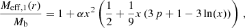
![Mathematical equation: $$ \begin{aligned} M_{\mathrm{eff} ,1}(x)&\equiv M_{\rm b} \left[ 1 + \alpha \int _0^x dx^{\prime } x^{\prime 2} \left( p_l - \frac{1}{a_0 r_{\mathrm{MOND} }}(\varphi _{\rm b}(x^{\prime }) + \hat{\Phi }_{\rm b}(x^{\prime }))\right)\right]\nonumber \\&= M_{\rm b} \left[1 + \alpha x^2 \left(\frac{1}{2} + \frac{1}{9} x \left(3p + 1 - 3 \ln (x)\right)\right) \right] \,, \end{aligned} $$](/articles/aa/full_html/2023/08/aa46025-23/aa46025-23-eq117.gif) (D.10)
(D.10)
where
 (D.11)
That is, p is the boundary condition for  for the choice l = rMOND.
This first order estimate can also be obtained more directly by setting φ = φb and  in the ghost condensate density Eq. (2). The advantage of the recursion formula Eq. (D.6) is that it is, at least conceptually, straightforward to improve on this approximation. And it allows to analytically estimate when the first order approximation breaks down by going to the next higher order, see Appendix J.5.
In the first order approximation, deviations from MOND are proportional to α. This is typically a small number for galaxies. To see this, first note that we typically have  (Skordis & Złosnik 2021). This is much larger than the MOND radius of galaxies, which typically satisfies rMOND ≲ 10 kpc. Thus, α is typically smaller than 10−4 for galaxies,
 (D.12)
In contrast, for galaxy clusters, the MOND radius can be large enough to give α = 𝒪(1).
Appendix E: Numerical solutions
In addition to the analytical approximation discussed above, we also made use of numerical solutions. To obtain these, we used the Julia package ‘OrdinaryDiffEq.jl‘ with the ‘AutoTsit5(Rosenbrock23())‘ method (Rackauckas & Nie 2017; Tsitouras 2011).
We again used the splits  and φ = φb + φc and numerically solved for
  and φc. The equations of motion are
 (E.1)
(E.1)
 (E.2)
(E.2)
where
 (E.3)
(E.3)
 (E.4)
(E.4)
 (E.5)
(E.5)
On the right-hand side of the φc equation, there is in general an additional term proportional to
 (E.6)
(E.6)
We left out this term since it vanishes for a baryonic point particle, ρb = Mbδ(x), which is what we consider here. To see that it vanishes, we first note that it vanishes outside r = 0 because of the factor ρb. For r → 0, we have ρb ∝ δ(r)/r2,  , and
, and  . The behavior of
  can, for example, be read off from our approximate analytical solution which is valid at r → 0. Thus, we can expand
  around φc′ = 0 and Eq. (E.6) becomes proportional to
 (E.7)
(E.7)
where we used that  scales as s−3/2 at large s while
  becomes constant.
We used a dimensionless length variable y = r/l with l = 1 kpc. We solved the equations in terms of v and u, which are obtained from φc and  , respectively, by rescaling and absorbing the constant μ/Q0,
 (E.8)
(E.8)
with A ≡ 10−7. We used the boundary conditions
 (E.9)
(E.9)
 (E.10)
The first follows from spherical symmetry, the second corresponds to a choice of chemical potential for the ghost condensate. When comparing the numerical solution to our analytical approximation, the following relation is useful,
 (E.11)
The logarithm accounts for the fact that p is defined for l = rMOND while we used l = 1 kpc for the numerical solution. To avoid numerical complications from the 1/r factor in the equations of motion, we did not impose these boundary conditions at r = 0 but at r = 10−5 kpc, corresponding to y = 10−5.
Appendix F: Oscillations, m2-fG-degeneracy
Above, we saw that the effective mass Meff – and thus also the acceleration – drops to zero at a finite radius. Beyond this radius, the acceleration begins to oscillate (Skordis & Złosnik 2021; Arkani-Hamed et al. 2007), see for example Fig. F.1. As discussed above, this oscillatory regime is potentially unstable since it involved negative energy densities and even negative masses. In this Appendix, we ignore this, keeping in mind that the oscillations might not be physical.
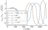 |
Fig. F.1. Total acceleration atot relative to the MOND-like acceleration |


The oscillations depend strongly on the combination m2/fG which multiplies the condensate density. This is illustrated in Fig. F.1 which shows multiple solutions with the same boundary condition and the same mass Mb but different values of the parameter m2/fG.
Indeed, in spherical symmetry, the total acceleration in the AeST model depends not on m and fG separately but only on the combination m2/fG. This is also illustrated in Fig. F.1 and can be understood from the integro-differential equation Eq. (C.5) that determines the total acceleration. Crucially, Eq. (C.5) depends only on the sum  but not on
  and φ separately.
Appendix G: Maximum radius of MOND-like behavior, optimal boundary conditions, relation to maximum of Meff
The AeST model deviates from MOND at large radii. Here, we discuss quantitatively at which radii these deviations occur and how large they are.
First, we point out that deviations from MOND are inevitable. By this we mean that, for given model parameters and a given baryonic mass Mb, one cannot push the deviations to arbitrarily large radii by judiciously adjusting the boundary condition. This can be seen by considering the effective mass Meff. If deviations from MOND are small, the zeroth order approximation Meff, 0 = Mb should be close to our first order approximation Meff, 1,
 (G.1)
(G.1)
where, again, p parametrizes the boundary condition, x = r/rMOND, and  . The general form of this function is that it approaches one for r → 0, has a maximum at some finite radius, and then drops to zero (see e.g., Fig. G.1). This definitely deviates from the zeroth order approximation (i.e., from MOND) when it drops to zero. And we can obviously make the radius where this happens arbitrarily large by making the boundary condition p arbitrarily large. So one might wonder whether we can avoid deviations from MOND by just making p arbitrarily large. But this is not possible because the larger p is, the more Meff deviates from MOND at its maximum. So there must be a finite optimal boundary condition p. For this optimal boundary condition, the radius up to which deviations from MOND stay small is maximized. We refer to this radius as rmax.
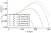 |
Fig. G.1. Total acceleration atot relative to the MOND-like acceleration |


More concretely, we considered the ratio of the acceleration  and its value without deviations from MOND, that is, we considered
  . If one allows this ratio to deviate from MOND by at most a fraction δ,
 (G.2)
(G.2)
That is, if one allows  to deviate from 1 by at most a fraction δ. Then, there is an optimal boundary condition p that allows this condition to be fulfilled up to a maximum possible radius rmax.
As we show in Appendix J.3, this optimal boundary condition is that for which  has the value 1 + δ at its maximum. We refer to this radius where
  reaches its maximum as rmaxratio. We illustrate the meaning of the quantities rmax, rmaxratio, and δ in Fig. 1.
Instead of  , we can also consider the total acceleration
  . This gives an analogous result: If we allow the total acceleration atot to deviate from MOND by at most a fraction δtot, then the optimal boundary condition is that for which
  has the value 1 + δtot at its maximum.
Strictly speaking, the optimal boundary conditions for  and
and  differ. At least for galaxies, however, the optimal boundary conditions are almost identical for both cases. Moreover, the maximizing radius and the value at this maximum are almost identical. This is shown in Appendix J.2. Thus, for our purposes, it does not matter much whether we consider the optimal boundary condition for
  or for atot.
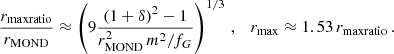
In Fig. G.2 we show the relation between the maximum allowed deviation from MOND δ and the maximum radius rmax up to which this condition can be fulfilled. For the numerical solutions, we found rmax by maximizing the radius where a solution first deviates by more than a fraction δ from MOND using the Julia package ‘Optim.jl‘ (Mogensen & Riseth 2018).
 |
Fig. G.2. Radius rmax up to which the acceleration |

As discussed above, for the optimal boundary conditions, the ratio  has the value 1 + δ at its first maximum. The radius rmaxratio where this maximum occurs is closely related to the radius rmax. This is illustrated in Fig G.3 which shows rmaxratio as a function of δ. This is very similar to Fig. G.2 just with the values on the y-axis a bit larger. In particular, rmaxratio corresponds to
 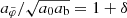 , while rmax corresponds to
  .
.
 |
Fig. G.3. Radius rmaxratio where the first maximum of the ratio |


In Appendix J.2 and Appendix J.4, we give an analytical estimate for the relation between δ, rmax, and rmaxratio. For galaxies, a good approximation is
 (G.3)
(G.3)
Thus, where this approximation is valid, the only difference between Fig. G.3 and Fig. G.2 is a factor 1.53 in the y-axis values.
Our estimate for rmax can be compared to a related estimate from Skordis & Złosnik (2021). There, the authors estimate that the AeST model acceleration is MOND-like up to a critical radius rc,
 (G.4)
(G.4)
This has the same scaling in rMOND and m as our estimate. However, our estimate improves on this in a few ways. First, the m2 factor in rc should be m2/fG. Otherwise, the estimate does not correctly take into account the difference between GN and  . Second, our version comes with worked out prefactors, including a parameter that controls how big deviations actually are.
We emphasize again that the maximum radius rmax – or the critical radius rc – corresponds to choosing boundary conditions that are optimal for reproducing MOND (given an allowed deviation δ). Galaxies are not guaranteed to reproduce MOND up to that radius. In general, galaxies will end up with boundary conditions different from the optimal one and deviate from MOND already at smaller radii.
In Fig. G.2 and Fig. G.3, we show our analytical approximation only where we analytically estimate that it deviates by at most q = 10% from the full solution. This validity estimate works by going to the next-higher order in our method for approximating Meff and then comparing to our first-order approximation, see Appendix J.5. Essentially, our approximation is valid for small deviations from MOND δ, but not for larger ones, as can already be guessed from Fig. G.1.
From Fig. G.2 and Fig. G.3 we see that more massive galaxies can remain close to MOND for longer than less massive galaxies. However, in the context of MOND, accelerations are often more important than radii. Thus, in Fig. 2, we show the minimum acceleration  corresponding to the maximum radius rmax. We see that the trend is now inverted due to the additional factor of Mb in ab. Less massive galaxies can have MOND-like behavior down to smaller accelerations than more massive galaxies.
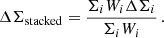
Appendix H: Stacking for weak lensing
In the weak-lensing analysis of Brouwer et al. (2021), the central quantity is the stacked excess surface density (ESD) profile ΔΣstacked. Stacking here means taking a weighted average over the galaxy sample. More specifically,
 (H.1)
(H.1)
where the Wi are weights, Σcrit is the critical surface density, ϵt is the ellipticity, and the factor 1 + μ calibrates the shear estimates. The ellipticity ϵt of a galaxy is the sum of its intrinsic ellipticity  and the tangential shear γt caused by weak lensing. The intrinsic ellipticities average to zero in a large sample, so that ΔΣstacked measures the tangential shear γt. For an individual lens and up to the calibration factor 1 + μ, the combination γtΣcrit is given by the ESD ΔΣ,
 (H.2)
(H.2)
where Σ(R) is the surface density corresponding to the lensing mass Mlens. Thus, for a galaxy sample with known surface densities, we can calculate ΔΣstacked by simply averaging the individual ESD profiles of each galaxy,
 (H.3)
(H.3)
The stacked ESD profile is linear in the surface densities Σi. These surface densities are calculated linearly from the density ρlens that produces the lensing mass Mlens. This lensing mass is defined by Φ′(r) = GNMlens/r2. In our case,
 (H.4)
(H.4)
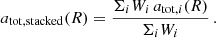
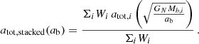
Thus, the stacked ESD profile is linear in  . As a consequence, the total acceleration atot inferred from the stacked ESD profile is just the weighted average of the total accelerations atot, i of each stacked galaxy,
 (H.5)
(H.5)
In order to calculate a stacked RAR, we should not stack at a fixed position R but at a fixed acceleration ab = GNMb/R2. So we should instead use
 (H.6)
(H.6)
For a fixed baryonic mass Mb, stacking in position space and acceleration space is equivalent.
We now illustrate how a stacked weak-lensing RAR in the AeST model might look like. For simplicity, we assume that all weights Wi are the same and we further assume that all galaxies have the same baryonic mass Mb. Essentially, we consider stacking a sample of galaxies that differ only in their boundary conditions. Then, we have
 (H.7)
(H.7)
where N is the number of galaxies in the sample.
One can also consider a large number of galaxies with boundary conditions p distributed uniformly in an interval [p1, p2]. Then, we can write
 (H.8)
(H.8)
As long as all accelerations atot, p(R) point in the usual direction, that is, as long as Meff is positive, this integral can be done analytically for our first order analytical approximation,
 (H.9)
(H.9)
where x = r/rMOND,  , and Meff(x, p) is our first order analytical approximation Eq. (D.10).
Appendix I: Higher-order terms in condensate density
The ghost condensate density from Eq. (2) is linear in the fields φ and  . In contrast, for their cosmological calculations, Skordis & Złosnik (2021) used a ghost condensate density including nonlinear corrections. Here, we discuss whether using the linearized form around galaxies is valid and explain our decision to do so.
In the full action, not assuming the quasi-static weak-field limit, the condensate density corresponds to a term
 (I.1)
(I.1)
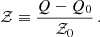
where Q = Aμ∇μϕ is a scalar combination of the normalized vector field Aμ and the scalar field ϕ. In the quasi-static weak-field limit, ϕ = Q0 ⋅ t + φ. The constant 𝒦2 is related to the mass parameter m by  .
.
Our expression for the ghost condensate Eq. (2) is linear because the function 𝒦(Q) is quadratic. Indeed, in the quasi-static weak-field limit,
 (I.2)
(I.2)
However, a quadratic function 𝒦(Q) cannot simultaneously satisfy cosmological constraints and support a MOND-like regime in galaxies (Skordis & Złosnik 2021). In particular, cosmological observations require that the ghost condensate’s equation of state w satisfies w ≲ 0.02 at a scale factor a = 10−4 (Ilić et al. 2021). But if we assume m2/fG ≲ 1/Mpc in order to have a MOND-like phenomenology around galaxies, w is too large. Indeed, using 0 < KB < 2 and fG < 1, (Skordis & Złosnik 2021)
 (I.3)
(I.3)
where H0 is the Hubble constant and Ω0 is the matter density parameter today. This is illustrated in Fig. I.1 which shows the cosmological ghost condensate density as a function of the scale factor a for m = 1 Mpc−1 (see the Q0/𝒵0 = 0 line, the parameter 𝒵0 is discussed below). We see that a dust-like evolution is possible at late times but not around a ∼ 10−4.
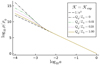 |
Fig. I.1. Cosmological ghost condensate density ρ as a function of the scale factor a relative to its density ρ0 today, at a = 1, for various values of the combination Q0/𝒵0. This is for m = 1 Mpc−1, KB = 0.1, H0 = 70 km s−1 Mpc−1, and Ω0 = 0.25. The ghost condensate follows a dust-like evolution only at late times. Larger values of m allow for dust-like evolution even at a = 10−4 but are in conflict with having MOND-like behavior around galaxies. |
To avoid this problem, Skordis & Złosnik (2021) introduced two alternative forms of 𝒦(Q),
 (I.4)
(I.4)
 (I.5)
(I.5)
where 𝒵0 is a constant and
 (I.6)
(I.6)
These suppress the equation of state at early times where 𝒵 is large and reduce to the quadratic 𝒦(Q) at small 𝒵.
In our galaxy-scale calculations above, we assumed the quadratic form of 𝒦(Q). This is justified only if 𝒵 is sufficiently small. To see whether or not this is the case, we first note that a typical value of 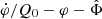 around galaxies is 10−7. Thus, a typical value of 𝒵 around galaxies is
 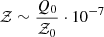 . That is, we can use the quadratic 𝒦(Q) as long as
 (I.7)
(I.7)
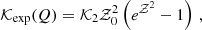
Interestingly, this condition is not satisfied, or only barely satisfied, for the explicit cosmological perturbation calculations in Skordis & Złosnik (2021). In particular, Skordis & Złosnik (2021) used Q0/𝒵0 = 108 for their example calculation using 𝒦cosh and Q0/𝒵0 = 1013 for 𝒦exp.
We nevertheless assume the quadratic form around galaxies for the following reasons. First, this seems to be what the authors of the model had in mind. After all, they use the quadratic form of 𝒦(Q) when deriving the action for the quasi-static weak-field limit (Skordis & Złosnik 2021).
Second, large values of Q0/𝒵0 do not seem to be required in order to satisfy cosmological constraints. Indeed, the constraint w ≲ 0.02 at a = 10−4 can easily be satisfied with a much smaller value of Q0/𝒵0. This is illustrated for 𝒦exp in Fig. I.2 which shows that Q0/𝒵0 = 𝒪(1) is sufficient.
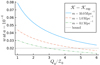 |
Fig. I.2. Equation of state at a = 10−4 as a function of Q0/𝒵0 for the exponential 𝒦(Q) function for various masses m. This is for KB = 0.1, H0 = 70 km s−1 Mpc−1, and Ω0 = 0.25. The dotted gray line shows the upper bound from Ilić et al. (2021). We note that m2 is the prefactor of 𝒦(Q). Thus, both the density and the pressure are proportional to m2 and this prefactor cancels in w. The dependence on m shown here comes from the constraint that the density parameter today is Ω0. |
Even if w satisfies w ≲ 0.02 at a = 10−4, it can be larger at later times and potentially violate observational constraints that apply at these later times. Indeed, w(a) is not a monotonous function, as is illustrated in Fig. I.3. Its maximum is set by Q0/𝒵0 and m controls at which scale factor a this maximum occurs. Still, we see from Fig. I.3 that Q0/𝒵0 = 𝒪(10) is sufficient for w to satisfy w ≲ 0.02 even at later times, thus easily satisfying the constraints at these times from Ilić et al. (2021). That is, these constraints can easily be satisfied with Q0/𝒵0 ≪ 107 which allows using the quadratic 𝒦(Q) around galaxies. We find a similar result for 𝒦cosh.4
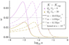 |
Fig. I.3. Equation of state at as a function of the scale factor a for the exponential 𝒦(Q) function for various masses m and ratios Q0/𝒵0. This is for KB = 0.1, H0 = 70 km s−1 Mpc−1, and Ω0 = 0.25. The dotted gray line shows the upper bound at a = 10−4 from Ilić et al. (2021). |
A third reason is that, if the nonlinearities of 𝒦exp or 𝒦cosh were to be important around galaxies, then either many galaxies would deviate very strongly from MOND or there would be almost no deviations from MOND at all. Both cases do not require a thorough investigation here. Strong deviations from MOND are ruled out by observations while pure-MOND predictions are already discussed elsewhere.
It remains to explain why 𝒦exp and 𝒦cosh have the effects described in the previous paragraph. We first consider 𝒦exp and 𝒦cosh with the parameter m having roughly the value we assumed above for the quadratic function 𝒦(Q), that is, m ∼ 1 Mpc−1. Then, as soon as nonlinearities become important, the condensate density is enhanced exponentially compared to the case of a quadratic 𝒦(Q). Thus, deviations from MOND set in exponentially earlier, that is, the radius rmax is exponentially smaller. For example, the oscillations discussed in Appendix F start at exponentially smaller radii. This is in conflict with, for example, the observed RAR which is MOND-like as discussed above.
One way out would be to make the prefactor m2 of 𝒦exp exponentially smaller to keep the ghost condensate from becoming large. Indeed, by choosing m2 sufficiently small, we can get rid of any significant deviations from MOND around galaxies. The predictions of the AeST model in this case are just those of MOND so do not require a special investigation.
A middle ground would be to make m2 exponentially smaller, but by just the right amount so that deviations from MOND set in on roughly galactic scales. However, the maximum radius rmax would still be exponentially sensitive to the galactic potential  . Thus, for galaxies with slightly larger
  , deviations from MOND still set in at an exponentially smaller radius compared to the quadratic 𝒦(Q). Galaxies with slightly smaller
 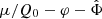 would perfectly follow the MOND predictions up to exponentially large radii. Thus, a significant fraction of galaxies should still deviate strongly from MOND which is not what is observed.
Appendix J: A few useful properties of Meff, 1(r)
In this appendix, we consider a few properties of the analytical first order approximation Meff, 1 from Eq. (D.10),
![Mathematical equation: $$ \begin{aligned} M_{\mathrm{eff} ,1}(r) = M_{\rm b} \left[1 + \alpha x^2 \left(\frac{1}{2} + \frac{1}{9} x \left(3 \, p + 1 - 3 \ln (x) \right) \right) \right]\,. \end{aligned} $$](/articles/aa/full_html/2023/08/aa46025-23/aa46025-23-eq201.gif) (J.1)
(J.1)
We sometimes write Meff instead of Meff, 1 for brevity.
J.1. Increasing functions of boundary condition
We first show that both  and
and  as well as their spatial derivatives are increasing functions of the boundary condition p. At least as long as Meff is positive. This technical result will be useful in Appendix J.3.
We first consider 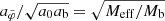 as a function of p. Both Meff(r) and
  are increasing functions of the boundary condition, that is, of p, for all r. This follows from α and r being positive. We then consider
  and
and  for radii where Meff is positive. In this case,
  is an increasing function of p everywhere because Meff is,
 (J.2)
(J.2)
The same holds for the spatial derivative  but it is a bit harder to see. We find
 (J.3)
(J.3)
which follows because r and Meff are positive.
We consider next, again assuming Meff > 0, the function
 (J.4)
(J.4)
where we defined H = Meff/Mb. Since Meff is an increasing function of the boundary condition p, the same holds for this function. The slope of this function with respect to x is also an increasing function of p, but this is again a bit harder to see. We have
 (J.5)
(J.5)
where we already inserted the explicit expressions for ∂pH and ∂p∂xH due to their simple form. It now suffices to show positivity of the following expression,
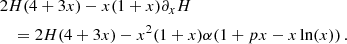 (J.6)
(J.6)
In general, this can be negative. However, here it cannot be due to our assumption that Meff is positive. To see this, we first use the definition of H to rewrite x(p − ln(x)) in terms of H,
 (J.7)
(J.7)
With this, we find
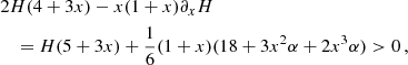 (J.8)
(J.8)
which completes the proof.
J.2. Maximum
We first consider the maximum of  . The maximum of both Meff(r) and
  is determined by
  . This condition can be written as
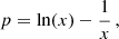 (J.9)
(J.9)
which can be solved in terms of the Lambert W function,
 (J.10)
Using this condition gives further for the maximum of  with value 1 + δ,
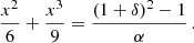 (J.11)
This can be solved exactly but the resulting expression is not particularly illuminating. The size of the right-hand side determines whether the x2 or the x3 term dominates. For large values, the x3 term dominates, for small values the x2 term dominates. For large right-hand sides, we have for the maximum
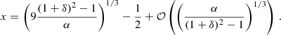 (J.12)
The boundary condition needed to obtain such a maximum is
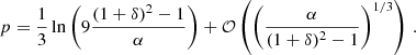 (J.13)
We consider next the maximum of  , that is, the maximum of the function
 (J.14)
assuming Meff > 0. The maximum of this function is both at a similar location and has a similar value as that of  – at least for galaxies. We first show that the maximum is at a similar location. To this end, we set the derivative with respect to x to zero, plug in x + δx where x is the maximizer of
  , expand to lowest order in δx, use H′(x) = 0, and solve for δx. This gives
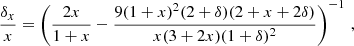 (J.15)
where we have additionally used Eq. (J.11), H(x) = (1 + δ)2, H″(x) = − (1 + x)α, and we have eliminated α by using Eq. (J.11), giving α = ((1 + δ)2 − 1)/(x2/6 + x3/9).
The simplest way to understand this expression is to plot it as a function of x for a number of values of δ. For δ ≪ 1, we have that |δx/x| is always smaller than 2.5%. For δ = 𝒪(1), it can become a bit larger. For example, up to δ = 1.5, we have that |δx/x| is always smaller than 5%. But even for extremely large values of δ, we have that |δx/x| is always smaller than 14.5%. Thus, the maximum of  is indeed at a similar location as that of
  .
.
Now we can evaluate the maximum value of the function Eq. (J.14), assuming that the maximizer is close to the one of  ,
,
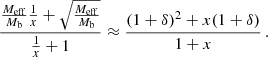 (J.16)
We can write this as
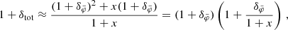 (J.17)
where 1 + δtot is the maximum value of Eq. (J.14) and  is the maximum of
  . We consider first small
  . Then, the factors relative to MOND are approximately the same in both cases, that is,
  . (But we note: δtot and δφ themselves might differ by up to a factor 2 for small x). When
  is not small, x is very large, see Eq. (J.11). At least for galaxies, which have α ≪ 1. Thus, the factors relative to MOND are again approximately the same in both cases – unless
  is very large. But for such large δ, our approximation is anyway no longer valid, see Appendix J.5.
J.3. Optimal boundary condition
We consider the ratio
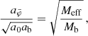 (J.18)
and require that it stays between 1 + δ and 1 − δ for some positive δ. One may wonder what the boundary condition is that allows this requirement to be fulfilled up to the maximum possible radius rmax. We refer to this as the optimal boundary condition. Here, we show that it is the boundary condition for which  has the value 1 + δ at its maximum, which we discussed in Appendix J.2.
To this end, we consider this solution for which  has the maximum value 1 + δ at some radius r1. This solution will have the value 1 − δ at some radius r2 > r1 since Meff drops to zero after the maximum. We refer to this solution’s boundary condition p as p1.
Here, we consider Meff > 0. When Meff < 0, the gravitational force in the AeST model points into the opposite direction from that in MOND. We are not interested in this regime here. Thus, we assume δ < 1 which implies Meff > 0.
Any solution with a boundary condition p larger than p1 has a larger value  everywhere (see Appendix J.1). This implies that such solutions must have
 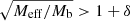 at r = r1. Thus, boundary conditions p larger than p1 cannot be optimal.
We then consider solutions with boundary condition p smaller than p1. Such solutions have a smaller value  and slope
  everywhere (see Appendix J.1). Thus, these solutions reach their maximum earlier than r1 and this maximum has a value smaller than 1 + δ. Starting at this lower maximum, such solutions then go to zero faster (since their slope is more negative). Thus, these solutions reach
 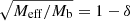 earlier than r2. Thus, smaller boundary conditions also cannot be optimal.
It follows that the optimal boundary condition is that which gives 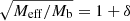 at the maximum of Meff. That is, we have p = p1.
The preceding argument implicitly considered negative condensate densities by considering radii beyond the radius where Meff is maximal. One may wonder whether anything changes when restricting solutions to have positive densities. But this is not the case, at least as long as we just cut off the solutions when the density reaches zero and do not continue them with something else (such as a Navarro-Frenk-White halo). The above argument can be straightforwardly adapted to this case.
Instead of  we could also consider the total acceleration relative to MOND. That is,
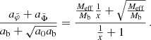 (J.19)
The argument above can be adapted to this case as well. That is, the optimal boundary boundary condition is that for which this total acceleration ratio has the maximum value 1 + δ.
The optimal boundary conditions for  are, in general, not the same as those for the total acceleration
  . However, in practice, they are very similar and give very similar deviations from MOND at very similar maximum radius. This follows from the properties of the maximum discussed in Appendix J.2.
J.4. Relation between rmax and rmaxratio
Here, we consider a solution that is optimal for some δ. As discussed above and as illustrated in Fig. 1, the radius rmaxratio is where the ratio  has its maximum value, namely 1 + δ, and rmax is the radius where this ratio drops to 1 − δ. Here, we consider the relation between these two radii. We argue that, usually, rmax is larger than rmaxratio by a fixed factor 1.53 for small δ.
Based on numerical examples, we first guess a factor around 1.5. Then, we calculate first-order corrections to this factor 1.5 and find that corrections are, in a certain regime, small. This confirms the validity of our initial guess. In addition, we find that the first-order corrections are universal and give a factor 1.53.
To find rmax, we must solve  . That is,
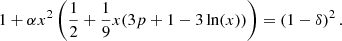 (J.20)
where x = rmax/rMOND. We write
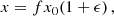 (J.21)
where x0 is the radius where this equation is satisfied with (1 + δ) instead of (1 − δ) on the right-hand side, that is to say it is the radius where Meff is maximal, that is, x0 = rmaxratio/rMOND. We later set f = 3/2 and let ϵ parametrize deviations from a factor 1.5 between rmax and rmaxratio, that is, later we find f(1 + ϵ)≈1.53.
We plug this expression for x back into the equation determining x, expand in ϵ, and solve for ϵ. Then, we eliminate first p and then α using the two conditions we know from x0 being a maximum, namely Eq. (J.9) and Eq. (J.11). This gives
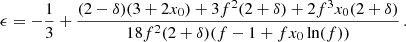 (J.22)
We now consider f = 3/2 and check whether or not ϵ is actually small. For large x0, we find
 (J.23)
The maximum radius x0 is large as long as δ/α ≫ 1, see Appendix J.2. For galaxies, we typically have α ≲ 10−4 (see Appendix G). Thus, this condition is fulfilled unless δ is extremely large. For such large δ, the first order analytical approximation for Meff is anyway no longer valid, as we show in Appendix J.5. Thus, for galaxies, the large-x0 result is typically valid.
If, in addition, we have δ ≪ 1, we find
 (J.24)
Thus,
 (J.25)
J.5. Validity of approximation
We now consider the validity of our first order approximation Meff, 1 for Meff from Eq. (D.10). Figure G.1 and other plots suggest that it is often a reasonable approximation but also that it becomes worse for larger deviations from MOND δ. Here, we estimate analytically when this approximation is valid.
To this end, we calculate the 2nd order approximation to Meff and check when the first and second orders deviate from each other. To facilitate a quantitative analytical estimate, we do not calculate the 2nd order approximation exactly. We make additional approximations and assumptions. The result should still be a reasonable estimate of when the first order approximation is valid.
The 2nd order approximation is obtained by plugging the first order approximation into the right-hand side of Eq. (D.6),
![Mathematical equation: $$ \begin{aligned} \frac{M_{\mathrm{eff,2} }(x)}{M_{\rm b}}&= \frac{M_{\mathrm{eff} ,1}(x)}{M_{\rm b}} - \alpha \int _0^x dx^{\prime } x^{\prime 2} \int _0^{x^{\prime }} dx^{\prime \prime } \left[ \frac{1}{x^{\prime \prime 2}} \left(\frac{M_{\mathrm{eff} ,1}(x^{\prime \prime })}{M_{\rm b}} - 1\right) \right.\nonumber \\&\qquad \quad ~~\left. + \frac{1}{x^{\prime \prime }} \left(s_{\mathrm{eff} ,1}(x^{\prime \prime }) \sqrt{\frac{|M_{\mathrm{eff} ,1}(x^{\prime \prime })|}{M_{\rm b}}}-1\right) \right] \,, \end{aligned} $$](/articles/aa/full_html/2023/08/aa46025-23/aa46025-23-eq263.gif) (J.26)
(J.26)
where the subscripts 1 and 2 refer to the first and second order approximations, respectively.
The double integrals in this expression can be done analytically for the part linear in Meff, 1. We find
 (J.27)
Below we express radii relative to where Meff, 1 has its maximum,
 (J.28)
We can also eliminate p by using the relation p = ln(xmr)−1/xmr. This gives
 (J.29)
We consider  between 0 and 1. The function
  grows from 0 to 1 in this
  interval. Thus, when xmr is large, that is, when rmaxratio is large compared to rMOND, this term will dominate, except at very small radii
  . Otherwise, the
  term dominates.
We now consider the remaining terms in Meff, 2/Mb, that is, those with  . Here, the double integrals are not straightforward to do analytically. Therefore, we make an additional approximation and we restrict ourselves to radii r before Meff, 1 reaches its maximum, that is, we only consider r ≤ rmaxratio. Concretely, we assume that
  grows linearly from 1 at r = 0 to its maximum 1 + δ at r = rmaxratio,
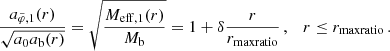 (J.30)
From Fig. 1 we see that this underestimates Meff, 1 at small radii and then overestimates it at larger radii toward rmaxratio. This is a rough approximation but we have verified numerically that it captures the validity of the first order approximation reasonably well. With this, we have
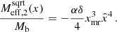 (J.31)
The remaining task is to sum  and
and  and determine when this sum deviates from Meff, 1. More specifically, we are interested mostly in
  so we are interested in the square root. We parametrize the deviation by a parameter q,
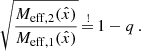 (J.32)
This relation determines the radius  where the 2nd order becomes important if we want to trust the first order approximation up to a fraction q.
Unfortunately, this equation is not straightforward to solve analytically. Thus, we make further approximations. First, we use the linear approximation 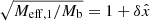 also in the denominator of Eq. (J.32) and the first term in
  . Second, we neglect the
  term in
  .
.
The reasoning behind the second of these approximations is the following. As argued above, the 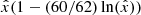 term is important only for large xmr. But in this case, the double-integral contributions to
  are anyway small compared to
  so it does not matter. Indeed,
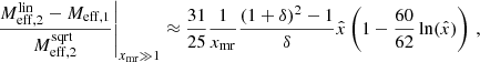 (J.33)
where we used 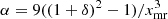 which is valid for xmr ≫ 1, see Eq. (J.11). Since
  and xmr ≫ 1, this ratio is small unless δ ≳ xmr. Thus, for our purposes this ratio is small. We are not interested in very large deviations from MOND δ which would be required for δ ≳ xmr ≫ 1.
Equation (J.32) then becomes
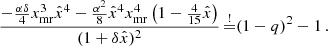 (J.34)
This is still not solvable analytically. Thus, our final approximation will be to neglect the  term. This is again a rough approximation but, as mentioned above, we have verified numerically that the result is reasonable. Thus, we need to solve
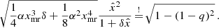 (J.35)
We finally find for the radius rapprox up to which the first order approximation is valid to within a fraction q,
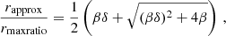 (J.36)
where
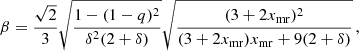 (J.37)
where we used Eq. (J.11) to eliminate α.
We note that we assumed r ≤ rmaxratio when deriving this estimate. Thus, if our expression for rapprox/rmaxratio is larger than 1, the first order approximation is valid up to at least rmaxratio but the precise value of rapprox/rmaxratio is not meaningful.
The most important implication of our estimate is that the first order approximation is good for small δ (except for extremely restrictive values of q). For larger δ, the approximation is worse. Explicitly, for small δ the quantity β scales as
 (J.38)
so that rapprox/rmaxratio scales as
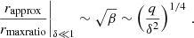 (J.39)
When δ is small, this ratio is large, so the first order approximation is valid. If we demand a better approximation (i.e., a smaller q), the radius rapprox becomes smaller.
In the opposite limit, δ ≫ 1,
 (J.40)
where the power 3 applies for sufficiently large xmr and the power 4 for sufficiently small xmr. In both cases does rapprox/rmaxratio tend to zero for large δ. So the first order approximation is not valid much.
All Tables
All Figures
|
Fig. 1. Numerical solution with the optimal boundary condition for δ = 0.05 (solid blue line). That is, the solution for which |
| In the text | |
|
Fig. 2. Acceleration |
| In the text | |
|
Fig. 3. RAR for different baryonic masses and boundary conditions for numerical solutions with fG/m2 = 0.99 Mpc2. The solid lines are for boundary conditions where |
| In the text | |
|
Fig. 4. Same as Fig. 3 but with all solutions truncated where the condensate density first drops to zero, that is, truncated where the solutions become potentially unstable. |
| In the text | |
|
Fig. 5. RAR for solutions with fixed baryonic mass Mb = 1011 M⊙ for various boundary conditions (green dotted lines) and the corresponding stacked RAR (solid red line). This is for fG/m2 = 0.99 Mpc2. The boundary conditions of the individual solutions are in the range 0.5 − 1.5 times the optimal boundary condition for δ = 0.05 with a step size of 0.1 times the optimal one. Solutions are cut off where the first of the individual solutions reaches atot = 0. We also show the analytically stacked RAR according to formula Eq. (H.9). |
| In the text | |
|
Fig. 6. Same as Fig. 5 but with all individual stacked solutions having positive condensate density. The individual solutions are for boundary conditions in the range 1.0 − 2.0 times the optimal boundary condition for δ = 0.05 with a step size of 0.1 times the optimal one. Solutions are cut off where the first of the individual solutions reaches ρc = 0. |
| In the text | |
|
Fig. 7. Observed weak-lensing RAR for ETGs and LTGs from Brouwer et al. (2021) with the stellar M/L* corrected to use the same stellar population model as the observed kinematic RAR (McGaugh 2022, priv. comm.) relative to the MOND prediction. This does not include the hot gas estimate from Brouwer et al. (2021). Here, we take aMOND = abνe(ab/a0) with |
| In the text | |
|
Fig. F.1. Total acceleration atot relative to the MOND-like acceleration |
| In the text | |
|
Fig. G.1. Total acceleration atot relative to the MOND-like acceleration |
| In the text | |
|
Fig. G.2. Radius rmax up to which the acceleration |
| In the text | |
|
Fig. G.3. Radius rmaxratio where the first maximum of the ratio |
| In the text | |
|
Fig. I.1. Cosmological ghost condensate density ρ as a function of the scale factor a relative to its density ρ0 today, at a = 1, for various values of the combination Q0/𝒵0. This is for m = 1 Mpc−1, KB = 0.1, H0 = 70 km s−1 Mpc−1, and Ω0 = 0.25. The ghost condensate follows a dust-like evolution only at late times. Larger values of m allow for dust-like evolution even at a = 10−4 but are in conflict with having MOND-like behavior around galaxies. |
| In the text | |
|
Fig. I.2. Equation of state at a = 10−4 as a function of Q0/𝒵0 for the exponential 𝒦(Q) function for various masses m. This is for KB = 0.1, H0 = 70 km s−1 Mpc−1, and Ω0 = 0.25. The dotted gray line shows the upper bound from Ilić et al. (2021). We note that m2 is the prefactor of 𝒦(Q). Thus, both the density and the pressure are proportional to m2 and this prefactor cancels in w. The dependence on m shown here comes from the constraint that the density parameter today is Ω0. |
| In the text | |
|
Fig. I.3. Equation of state at as a function of the scale factor a for the exponential 𝒦(Q) function for various masses m and ratios Q0/𝒵0. This is for KB = 0.1, H0 = 70 km s−1 Mpc−1, and Ω0 = 0.25. The dotted gray line shows the upper bound at a = 10−4 from Ilić et al. (2021). |
| In the text | |
Current usage metrics show cumulative count of Article Views (full-text article views including HTML views, PDF and ePub downloads, according to the available data) and Abstracts Views on Vision4Press platform.
Data correspond to usage on the plateform after 2015. The current usage metrics is available 48-96 hours after online publication and is updated daily on week days.
Initial download of the metrics may take a while.