| Issue |
A&A
Volume 675, July 2023
|
|
|---|---|---|
| Article Number | A72 | |
| Number of page(s) | 14 | |
| Section | Cosmology (including clusters of galaxies) | |
| DOI | https://doi.org/10.1051/0004-6361/202346210 | |
| Published online | 03 July 2023 | |
The cosmic radio dipole: Bayesian estimators on new and old radio surveys
1
Max-Planck Institut für Radioastronomie, Auf dem Hügel 69, 53121 Bonn, Germany
e-mail: wagenveld@mpifr-bonn.mpg.de
2
Fakultät für Physik, Universität Bielefeld, Postfach 100131, 33501 Bielefeld, Germany
Received:
21
February
2023
Accepted:
24
May
2023
The cosmic radio dipole is an anisotropy in the number counts of radio sources and is analogous to the dipole seen in the cosmic microwave background (CMB). Measurements of source counts of large radio surveys have shown that, although the radio dipole is generally consistent in direction with the CMB dipole, the amplitudes are in tension. These observations present an intriguing puzzle, namely the cause of this discrepancy, with a true anisotropy breaking with the assumptions of the cosmological principle, invalidating the most common cosmological models that are built on these assumptions. We present a novel set of Bayesian estimators to determine the cosmic radio dipole and compare the results with those of commonly used methods applied to the Rapid ASKAP Continuum Survey (RACS) and the NRAO VLA Sky Survey (NVSS) radio surveys. In addition, we adapt the Bayesian estimators to take into account systematic effects known to influence large radio surveys of this kind, folding information such as the local noise floor or array configuration directly into the parameter estimation. The enhancement of these estimators allows us to greatly increase the number of sources used in the parameter estimation, yielding tighter constraints on the cosmic radio dipole estimation than previously achieved with NVSS and RACS. We extend the estimators further to work on multiple catalogues simultaneously, leading to a combined parameter estimation using both NVSS and RACS. The result is a dipole estimate that perfectly aligns with the CMB dipole in terms of direction but with an amplitude that is three times as large, and a significance of 4.8σ. This new dipole measurement is made to an unprecedented level of precision for radio sources, which is only matched by recent results using infrared quasars.
Key words: large-scale structure of Universe / galaxies: statistics / radio continuum: galaxies
© The Authors 2023
 Open Access article, published by EDP Sciences, under the terms of the Creative Commons Attribution License (https://creativecommons.org/licenses/by/4.0), which permits unrestricted use, distribution, and reproduction in any medium, provided the original work is properly cited.
This article is published in open access under the Subscribe to Open model.
Open Access funding provided by Max Planck Society.
1. Introduction
The cosmic microwave background (CMB) and the structures seen therein reveal information about the large-scale structure in the Universe. In addition to the well-studied low-level (ΔT/T ∼ 10−5) anisotropies, there is a larger anisotropy seen in the CMB known as the cosmic dipole (ΔT/T ∼ 10−3), an effect attributed to the movement of the Solar System with respect to the CMB restframe. The velocity of the Solar System as derived from the amplitude of the CMB dipole is v = 369.82 ± 0.11 km s−1 (Aghanim et al. 2020), assuming that the dipole is entirely caused by the motion of the observer with respect to the CMB.
Ellis & Baldwin (1984) first proposed a way to measure the dipole in the number counts of radio sources, as the radio population outside of the Galactic plane mostly consists of extragalactic sources that are expected to be part of and to trace large-scale structure. The first significant measurement of the cosmic radio dipole1 was reported by Blake & Wall (2002) using the National Radio Astronomy Observatory (NRAO) Very Large Array (VLA) Sky Survey (NVSS, Condon et al. 1998); their result agreed with the CMB dipole within uncertainties. However, subsequent studies using the NVSS found the amplitude of the cosmic radio dipole to be significantly larger than that of the CMB dipole. Singal (2011) found a radio dipole to be four times larger, which was corroborated by Rubart & Schwarz (2013), and both measurements were obtained with a 3σ significance. In addition to the NVSS measurement, the cosmic radio dipole was measured with other radio surveys, such as the Westerbork Northern Sky Survey (WENSS, Rengelink et al. 1997), the Tata Institute for Fundamental Research (TIFR) Giant Metrewave Radio Telescope (GMRT) Sky Surveys first alternative data release (TGSS ADR1, Intema et al. 2017), and the Sydney University Molonglo Sky Survey (SUMSS, Mauch et al. 2003). Though depending on the survey and employed estimator, the amplitude of the radio dipole is consistently larger than the amplitude of the CMB dipole (see Siewert et al. 2021, for an overview), while the direction of the radio dipole remains consistent with that of the CMB, albeit with considerable uncertainty. It has been argued that failing to take into account the evolution of the spectral index, the magnification bias, or the luminosity function of the source population over cosmic time can potentially bias the radio dipole (Dalang & Bonvin 2022; Guandalin et al. 2022), although so far this evolution has not been observed (e.g. Böhme et al. 2023).
Most significant are the results from Secrest et al. (2021, 2022), which find a dipole amplitude over twice that of the CMB at a significance of 4.9σ using Wide-field Infrared Survey Explorer (WISE, Wright et al. 2010) measurements of quasars. Secrest et al. (2022) perform a joint analysis of NVSS radio galaxies and WISE quasars, with a resulting significance of 5.1σ. A Bayesian estimator based on Poisson statistics was recently utilised by Dam et al. (2022) for the first time to measure the cosmic radio dipole with the WISE quasar sample from Secrest et al. (2021), yielding a dipole amplitude 2.7 times larger than the CMB dipole with a significance of 5.7σ. Ultimately, a discrepancy between a dipole in the CMB and other observables points to an unknown effect on the data, which is increasingly unlikely to be systematic among all the different probes, as the NVSS and WISE samples for example are independent of one another, both in terms of source population and systematic effects. This points to an unexpected anisotropy in the large-scale structure of the Universe, something which breaks with the core assumptions of the cosmological principle. If genuine, this anisotropy poses a major problem for cosmologies that are based on the Friedmann-Lemaître-Robertson-Walker metric, such as Λ-CDM.
One problem that remains persistent, even with ever larger datasets, is a lack of homogeneity caused by systematic effects that influence the data. Systematic effects that are unaccounted for can greatly bias dipole estimates, and so conservative cuts in the data must be made to eliminate biases as much as possible. Already in the first measurement of the cosmic radio dipole using the NVSS (Blake & Wall 2002), a persistent systematic effect was identified that causes large differences in source density as a function of declination, inducing an artificial north–south anisotropy in the data. To eliminate this effect and avoid biasing dipole estimates, conservative cuts in flux density have to be made in such catalogues, which greatly reduces the number of usable sources.
Wagenveld et al. (2023) presented a deep analysis of ten pointings from the MeerKAT Absorption Line Survey (Gupta et al. 2016), with a focus on mitigating biases that could affect a measurement of the cosmic radio dipole. Being able to account for systematic effects allows less strict flux density cuts to be made, increasing the homogeneity of the catalogues and the number of sources that can be used for a dipole estimate. This approach was made possible by having direct access to meta data and data products within the processing steps of the survey from calibration to imaging and source finding, which is commonly not the case in dipole studies. In the present work, we approach this problem from the outside, and show how dipole estimates can be improved with the information present in modern radio catalogues. We present new dipole estimators, constructing likelihoods for estimating dipole parameters that can take this information into account, as well as an estimator that combines different catalogues for an improved dipole estimate. Given the proper information, these estimators are able to account for systematic effects on number counts in radio surveys and remove the need to cut large amounts of data.
This paper is organised as follows. In Sect. 2, we describe the statistics of radio source counts and the dipole effect. In Sect. 3, we introduce the estimators that will be used to infer the radio dipole parameters using the data sets described in Sect. 4. The results obtained are given in Sect. 5. The implications of our results are discussed in Sect. 6, along with some caveats. In Sect. 7, we summarise the findings of our study.
2. Radio source counts and the dipole
The majority of bright sources at radio wavelengths outside of the Galactic plane are active galactic nuclei (AGN) and have a redshift distribution that peaks at z ∼ 0.8 (e.g. Condon & Ransom 2016). As such, radio sources are expected to trace the background, and should therefore comply with isotropy and homogeneity on the largest scales. Following the cosmological principle, the surface density of sources should therefore be independent of location on the sky. The naive expectation is a distribution of radio sources that are independent, identical, and point-like, which defines a Poisson point process. By discretising the sky into regions of finite size, the number of sources per region will follow a Poisson distribution. The probability density distribution

is entirely parametrised by the variable λ, which describes both the mean and variance of the distribution. In actual radio data, some deviations from a perfect Poisson distribution are expected due to clustering and the presence of sources with multiple components. The severity of these effects depends largely on factors such as survey depth, angular resolution, and observing frequency, and is therefore difficult to assess without a thorough analysis of the survey. Such an analysis is beyond the scope of this work, but would follow a structure similar to that of Siewert et al. (2020), who demonstrate for the LOFAR Two-Metre Sky Survey first data release (LoTSS DR1, Shimwell et al. 2019) that the distribution of source counts converges to a Poisson distribution if applying stricter flux density cuts. For the analysis presented in this work, we assume that the effects of clustering and multi-component sources are negligible on a dipole estimate.
The spectral features and number count relations of typical radio sources make them uniquely suitable for a dipole measurement. For most sources, the dominant emission mechanism at radio wavelengths is synchrotron radiation, the spectral behaviour of which is well described by a power law,

with a characteristic spectral index α. For synchrotron emission, the typical value of α is around 0.75 (e.g. Condon 1992), and this value has been assumed for most dipole studies at radio wavelengths (Ellis & Baldwin 1984; Rubart & Schwarz 2013; Siewert et al. 2021). Furthermore, the number density of radio sources follows a power-law relation with respect to the flux density S above which the counts are taken,
The value of x can differ between surveys depending on the choice of flux density cut and frequency of the catalogue, but usually takes values of 0.75−1.0.
In the frame of the moving observer, given a velocity β = v/c, a systemic Doppler effect shifts the spectra of sources, which affects the flux density of these sources. Additionally, sources are Doppler boosted from the point of view of the moving observer, which further affects the observed flux density of sources. Depending on their angular distance from the direction of motion θ, the flux densities are shifted by

Thus, given a flux-limited survey of radio sources, more sources appear above the minimum observable flux in the direction of the motion, and less will appear in the opposite direction. Finally, relativistic aberration caused by the motion of the observer shifts the positions of sources towards the direction of motion, causing a further increase in number counts in the direction of motion,
As the fluxes and positions of the sources are shifted, we observe the dipole as an asymmetry in the number counts of radio sources. Combining these effects to first order in β, and therefore assuming that v ≪ c, shows the expected dipole amplitude for a given survey:

![$$ \begin{aligned}&\mathcal{D} = [2 + x(1+\alpha )]\beta . \end{aligned} $$](/articles/aa/full_html/2023/07/aa46210-23/aa46210-23-eq7.gif)
As such, we can directly infer the velocity of the observer by measuring the dipole effect on the number counts of sources. However, this necessitates the assumption that the dipole is entirely caused by the motion of the observer. Given the observed discrepancy between the CMB dipole and the radio dipole, it would be equally appropriate to assume that part of the observed radio dipole is caused by a different (and as-of-yet unknown) effect.
Given a dipole characterised by Eq. (7), different dipole amplitudes 𝒟 are expected to be seen depending on the data set being used. Though aberration always has an equal effect, the effect of Doppler shift is determined by the spectral index α of the sources, and both this and the Doppler-boosting effect depend on the flux distribution of sources, which is characterised by the power-law index x. Single values are most often assumed for these quantities, from which the expectation of the dipole amplitude can be derived. These quantities will differ at least between different surveys, and so we derive them for each survey separately. Although the entire flux distribution of any survey cannot be characterised with a single power-law relation, the dipole in number counts is caused by sources near the flux density threshold, making the power-law fit near this threshold the most appropriate choice for deriving x. For the entire range of frequencies considered in this work, we assume a spectral index of α = 0.75, considering the synchrotron emission of radio sources which dominates the spectrum of radio sources below 30 GHz (Condon 1992).
3. Dipole estimators
Different types of estimators have been used to measure the cosmic radio dipole, which for the most part yield consistent results. Most commonly used are linear and quadratic estimators (e.g. Singal 2011; Rubart & Schwarz 2013; Siewert et al. 2021). Linear estimators essentially sum up all source positions, and therefore, by design, point towards the largest anisotropy in the data. However, the recovered amplitude from linear estimators is inherently biased. Furthermore, because of the sensitivity of linear estimators to anisotropies, any gaps or systematic effects in the data can introduce biases in the estimate of the dipole direction. To avoid biasing the estimator with respect to dipole direction, a mask must be created such that the map remains point symmetric with respect to the observer, or a ‘masking correction’ must be applied (e.g. Singal 2011; Rubart & Schwarz 2013). Consequently, missing data features such as the Galactic plane must be mirrored to maintain symmetry, removing even more data. The quadratic estimator compares expected number counts with a model, providing a chi-squared test of the data with respect to a model of the dipole (e.g. Siewert et al. 2021). The best-fit dipole parameters are then retrieved by minimising χ2. Though the cost is the imposition of a dipole model on the data, the estimate is not biased by the ubiquitous spatial gaps in the data of radio surveys.
Both aforementioned estimators are sensitive to anisotropies in the data introduced by systematic effects. Most commonly, these systematic effects influence the sensitivity of the survey in different parts of the sky, meaning the most straightforward solution is to cut out all sources below some flux density. However, given this assessment, we might expect information in terms of the sensitivity of the survey in different parts of the sky to help alleviate these biases. The new generation of radio surveys provides catalogues with a wealth of information, including the local root-mean-square (rms) noise, which we exploit in this work.
To improve sensitivity to the dipole, several attempts have been made to combine different radio catalogues. Both Colin et al. (2017) and Darling (2022) worked on combining different radio surveys, using different techniques to deal with systematic differences between the catalogues. Here, we provide an alternative method to combine catalogues for increased sensitivity to the dipole, while accounting for systematic differences between the catalogues.
3.1. Quadratic estimator
To control for differences in pixelation and masking strategies between this and previous works, introducing a new estimator warrants a comparison with known methods of dipole estimation. The quadratic estimator is the closest analogy to the Poisson estimator used here to produce our main results in that it is insensitive to gaps in the data. Its effectiveness and results on multiple large radio surveys are presented in Siewert et al. (2021). The quadratic estimator is based on the Pearson’s chi-squared test, minimising
where the dipole model is written as
Here, the dipole amplitude on a given cell is given by the inner product between the dipole vector d and the unit vector pointing in the direction of the cell  , with
  . In addition to the dipole vector, the monopole ℳ is a free parameter, for which the mean value of all cells
  is a good initial estimate. The χ2 test is agnostic to the actual distribution of the data, but a dipole model is imposed on the data. This can give rise to misleading results if there are anisotropies in the data –such as those caused by systematic effects– on large enough scales and with sufficiently large amplitude to influence the fit. This can generally be assessed with the reduced χ2, which should take a value of around unity if the fit is good.
3.2. Poisson estimator
In the dipole estimators used in previous works, no explicit assumption was made as to the shape of the distribution of sources. A Gaussian distribution can be a valid assumption for a source distribution, although it has an additional degree of freedom compared to Poisson and is less valid if cell counts are low. However, as we do not know a priori how many sources we have, and as we do not commit to a cell size for which we count sources, we choose to assume a Poisson distribution for our cell counts. The Poisson probability density function is given by Eq. (1), and depends on the mean of the distribution λ, which is equal to the monopole ℳ in the absence of anisotropies. To account for the effect of the dipole, we introduce a dipole model equivalent to Eq. (9),

In order to estimate the dipole parameters, we maximise the likelihood, which is given by
Maximising the likelihood through posterior sampling has the key advantage of immediately yielding the uncertainties on the derived parameter values. This removes the necessity for null-hypothesis simulations as performed by for example Rubart & Schwarz (2013) and Secrest et al. (2021, 2022). This estimator was recently used by Dam et al. (2022), who showed that it provides tighter constraints on the dipole than previously used methods.
3.3. Poisson-rms estimator
While a survey can be influenced by many different systematic effects, we can assert that the net effect is different sensitivity of the survey at different parts of the sky, leading to anisotropic number counts. Therefore, we assume that all systematic effects that impact source counts in fact influence local noise, thereby causing the source density to vary across the survey. If the survey has sensitivity information in each part of the sky, the impact can be simply modelled by introducing additional variables to the model. So long as a detection threshold is consistently applied to the entire survey, the lower flux density limit will be linearly related to the local rms noise. Consequently, taking into account the dipole and the power law describing number counts, we can model the mean counts in the Poisson estimator as
where σ is the rms noise of the cell, x is the power-law index of the flux distribution, and σ0 is a reference rms value that scales the power law and explicitly ensures λ is dimensionless. The value of σ0 does not influence any parameters except for the monopole ℳ, which will take a value closest to the mean cell count  when taking σ0 as equal to the median rms noise over all cells. As the dipole amplitude depends on the power-law index of the flux distribution near the flux limit, the variation in the rms noise should be small enough that it can be adequately described with a single value. We expect a linear relation between the flux density limit and the local noise, as the detection threshold for most surveys is some multiple of the noise; usually 5σ. Maximising the likelihood given by Eq. (11) while inserting Eq. (12) for λ can therefore yield the best-fit dipole and power-law parameters.
3.4. Multi-Poisson estimator
Hoping to remove any systematic effects stemming from the incomplete sky coverages of individual radio surveys, Darling (2022) combined the Rapid Australian Square Kilometre Array Pathfinder (ASKAP) Continuum Survey (RACS, McConnell et al. 2020) and the VLA Sky Survey (VLASS, Lacy et al. 2020), finding a dipole that, surprisingly, agrees with the CMB in both amplitude and direction, though with large uncertainties. Secrest et al. (2022) note two inherent problems to this approach. Not only might selecting catalogues at different frequencies select different spectral indices, invalidating the assumption of a common dipole amplitude, but combining the catalogues in such a way ignores systematic effects that can vary between catalogues. Indeed, it is most likely the second factor that plays the most important role, as factors such as observing frequency, array configuration, and calibration can all impact the number counts within a survey in ways that are difficult to predict; this is even more true for independent surveys.
Bearing this in mind, we approach the combination of any two catalogues in a different way. We do not make any attempt to unify the catalogues by matching, smoothing, or creating a common map. Rather, we take both catalogues as independent tracers of the same dipole, allowing the two catalogues to have a different monopole amplitude ℳ. In the Poisson estimator, we therefore estimate ℳ separately for each catalogue, turning the likelihood into
Any dipole estimates with this likelihood benefit if the (expected) dipole amplitudes of the two catalogues are similar. However, any differences will be absorbed into the overall error budget by virtue of the sampling algorithm. Once again, the likelihood can be maximised through posterior sampling, yielding the best-fit dipole results as well as the monopoles ℳ1 and ℳ2 for both surveys.
3.5. Priors and injection values
For efficient parameter estimation through posterior sampling, proper priors must be set. While priors on parameters can take on many shapes based on prior knowledge, we take flat priors on all parameters. This only leaves us to define the extent of the probed parameter space, as well as the initial guesses to serve as a starting point for the posterior sampling. In terms of dipole parameters, we separately infer dipole amplitude 𝒟, as well as the right ascension and declination of the dipole direction. We expect the dipole amplitude to take values of around 10−2, but to allow for more variation, the prior on the dipole amplitude is set to π(𝒟) = 𝒰(0, 1). Any point in the sky can represent the dipole direction, and so logically the priors cover the entire sky: π(RA) = 𝒰(0, 360) and π(Dec) = 𝒰(−90, 90). As an initial guess for these parameters, we inject the approximate expected dipole parameters from the CMB: 𝒟 = 4.5 × 10⁻³, RA = 168°, Dec = −7°.
Additionally, the parameters of the distribution of number counts are also estimated. In the basic Poisson case, this is represented by the monopole ℳ. As the dipole is not expected to meaningfully impact this value, a good initial guess of the monopole is the mean of all cell counts  . As the real monopole is likely close to this value, we choose the prior
  . For the Poisson-rms estimator, both a monopole ℳ and power-law index x are estimated. Before the estimation, we fit a power law to the cell counts in order to ontain initial estimates ℳinit and xinit, which also function as the initial guesses for these parameters. The initial monopole estimate informs the prior as we use π(ℳ) = 𝒰(0, 2ℳinit). For the power-law index x, a value of around 0.75−1.0 is always expected, and so we take the prior π(x) = 𝒰(0, 3).
4. Data
Given the estimators introduced in Sect. 3, there are a multitude of available radio catalogues to possibly make use of for a dipole estimate. To maintain the focus of our approach, we use NVSS and RACS, two catalogues that cover the full sky when combined, but have been processed in very different ways given the respective eras in which they were produced. Given the introduction of novel estimators, the NVSS is the logical choice for verification, providing a baseline as the most thoroughly studied catalogue in terms of dipole measurements. The choice of RACS for the second catalogue is straightforward; not only does it complement NVSS in terms of sky coverage, but the inclusion of sensitivity information in the catalogue makes it suitable for testing the Poisson-rms estimator described in Sect. 3.3. The complementary sky coverage of the two catalogues also provides the best testing ground for the Multi-Poisson estimator described in Sect. 3.4.
4.1. NVSS
The NVSS (Condon et al. 1998) is one of the most well-studied surveys in terms of dipole measurements, and as such is well suited for verifying novel dipole estimators. It covers the whole sky north of −40° declination, and has a central frequency of 1.4 GHz and an angular resolution of 45″. The complete catalogue includes the Galactic plane and contains 1 773 484 sources.
An important feature of the NVSS catalogue is that, for observations below a declination of −10° and above a declination 78°, the VLA DnC array configuration was used for observations, while the VLA D configuration was used for the rest of the survey. This affects the number counts at those declinations. The left plot of Fig. 1 shows the source density of NVSS as a function of declination for different flux density cuts. The impact of the different array configurations can be clearly seen at lower flux densities. At only around 15 mJy, the source density becomes homogeneous, and so for an unbiased dipole analysis we choose to exclude all sources with a flux density below 15 mJy, which is a commonly applied flux density cut (e.g. Singal 2011; Siewert et al. 2021). Even after this cut, some areas with significantly high source counts are present in the data. We mask these areas as specified in Table 1 for the dipole estimate.
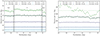 |
Fig. 1. Source density of NVSS (left) and RACS (right) as a function of declination for different flux density cuts. For the NVSS, we show the boundaries where different array configurations are used. In both cases, the catalogues can be seen to be inhomogeneous at low flux densities. |
Areas in NVSS masked due to high source density.
With a flux density cut at 15 mJy, we fit a power law to the lower end of the flux distribution of sources and find a power-law index of x = 0.85. Additionally taking α = 0.75 and taking the velocity from the CMB into account (Eq. (7)), this sets the expectation of the dipole amplitude to 𝒟 = 4.30 × 10⁻³.
4.2. RACS
RACS is the first large survey carried out using the Australian Square Kilometre Array Pathfinder (ASKAP), covering the sky south of +40° declination. Observations are carried out with a central frequency of 887.5 MHz and images are smoothed to a common angular resolution of 25″. The first data release of RACS in Stokes I is described in Hale et al. (2021), and the catalogue used in this work is the RACS catalogue with the Galactic plane removed, containing 2 123 638 sources. Source finding in the images has been done with the Python Blob Detector and Source Finder (PyBDSF, Mohan & Rafferty 2015), which provides a wealth of information on each source. Most importantly, the root-mean-square (rms) noise at the position of each source is present in the noise column of the catalogue, and we use this in the Poisson-rms estimator approach.
The right plot of Fig. 1 shows the source density of RACS as a function of declination for different flux density cuts. Even though there is no change in array configuration as with NVSS, there is a clear gradient in source density, where a greater number of sources are detected at lower declinations. Once again, the catalogue becomes homogeneous at flux densities of around 15 mJy, and so we exclude all sources below this flux density, as with NVSS. Even after this cut, some areas with significantly low source counts are present in the data. These areas appear just above the celestial equator. We mask these areas as specified in Table 2 for the dipole estimate.
Areas in RACS masked due to low source density.
With a flux density cut at 15 mJy and the other masks applied, we fit a power law to the lower end of the flux distribution of sources of RACS and find a power-law index of x = 0.82. Taking once again α = 0.75, this sets the expectation of the dipole amplitude to 𝒟 = 4.24 × 10⁻³.
4.3. Common masks and pixelation
In order to avoid biases to the data, we adopt a masking scheme that uses the same principles for both NVSS and RACS. As mentioned previously, surveys are generally not homogeneous at the lowest flux densities due to variations in the noise, and so we must choose a lower flux density threshold appropriate for the survey. As described above, for both NVSS and RACS we choose a flux density threshold of 15 mJy. To avoid counting Galactic sources or Galactic extended emission, we exclude the Galactic plane. Due to problems with source finding in the Galactic plane, it is already removed in the RACS catalogue, excluding all sources with |b|< 5°. For NVSS, overdensities from the Galactic plane extend further out, and we exclude all sources with |b|< 7°. Finally, we expect that the brightest sources in a survey push to the limit of the dynamic range, which introduces artefacts around bright sources. Due to differences in source-finding methods between the two catalogues, this increases counts around bright sources in NVSS, but decreases counts around bright sources in RACS. In both cases, the local source density is affected, and therefore we remove all sources within a radius of 0.3° around any source brighter than 2.5 Jy.
After masking data, we use the Hierarchical Equal Area isoLatitude Pixelation (HEALP IX, Górski et al. 2005)2 scheme to divide the sky into cells of equal size. HEALP IX allows the flexibility of choosing the number of cells over the whole sky, with the base and minimum value being 12 pixels. The resolution parameter Nside determines the number of pixels by  . We choose two resolutions for our experiment, Nside = 32 and Nside = 64, which have pixel sizes of 110′ and 55′ on a side, respectively. For measuring number counts, each cell holds the number of sources detected within the confines of the cell. To avoid edge effects resulting from pixels covering data only partially, all pixels that have a neighbouring pixel with zero sources are also set to zero. Finally, all pixels with a value of zero are masked to ensure that these pixels are not taken into account during dipole estimation. The HEALP IX maps of NVSS and RACS with Nside = 32, with flux density cuts and masks applied, are shown in Fig. 2. For the Poisson-rms estimator, the local noise is determined per HEALP IX cell by taking the median rms of all the sources within the cell.
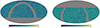 |
Fig. 2. Number counts for NVSS (left) and RACS (right) in equatorial coordinates, in Nside = 32 HEALP IX maps with masks and a flux density cut of 15 mJy applied. |
4.4. Simulations
In addition to the survey data sets of NVSS and RACS, we create a catalogue of simulated sources with a dipole effect to test the validity of the estimators. To do this, we uniformly populate the sky with sources, and assign a rest flux density Srest according to the power law
where 𝒰 is a uniform distribution between 0 and 1, Slow is the lower flux density limit at which sources are generated, and x the power-law index of the flux density distribution. We transform the rest flux densities and positions of sources by applying relativistic aberration, Doppler shift, and Doppler boost as expressed in Eqs. (4) and (5).
We add Gaussian noise to the flux densities of the sources, generating a larger sample of sources and simulating source extraction by only including sources with S/N > 5 in the final catalogue. This naturally adds the effect of Eddington bias to the sample, which is expected to be present in real source catalogues. For a realistic distribution, the local noise variation is taken from the RACS Nside = 32 rms map, idealising by assigning the rms of a cell to all sources in that cell. Additionally, we simulate false detections by generating sources with the same flux distribution that are not affected by the dipole. These sources consist of 0.3% of the total catalogue, which is the percentage reported for the RACS catalogues (Hale et al. 2021).
All sources are simulated with a spectral index of 0.75, and the power law used to generate the flux distribution has x = 1. We apply the dipole effect assuming the direction derived from the CMB dipole, (RA, Dec) = (170° , − 10° ), but with an increased velocity of v = 1107 km s−1 to ensure that a sensitivity to the dipole is reached that is similar to that of NVSS and RACS, with similar monopole values. This sets the expectation of the dipole to 𝒟 = 1.5 × 10⁻².
5. Results
Using the described estimators, we estimate the dipole parameters for NVSS and RACS. The results are summarised in Table 3, with dipole directions shown in Fig. 3 and dipole amplitudes shown in Fig. 4. To estimate the best-fit parameters, for the quadratic estimator, we minimise χ2 using LMFIT (Newville et al. 2016). The reduced χ2-values are reported in Table 3. For the Poisson estimators, we use the Bayesian inference library BILBY (Ashton et al. 2019), which provides a convenient and user-friendly environment for parameter estimation. We maximise the likelihood using Markov chain Monte Carlo (MCMC) sampling with EMCEE (Foreman-Mackey et al. 2013). The scripts used to obtain these results are available on GitHub3 and an immutable copy is archived in Zenodo (Wagenveld 2023).
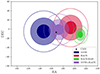 |
Fig. 3. Best-fit dipole directions for the Poisson estimator of NVSS (blue), RACS (red), RACS with rms power law (green), and NVSS+RACS (purple) compared with the CMB dipole direction (black star). Different transparency levels represent 1σ, 2σ, and 3σ uncertainties. In all cases, results from the Nside = 32 HEALPix map are shown. |
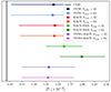 |
Fig. 4. Best-fit dipole amplitudes with 3σ uncertainties for the Poisson estimator of NVSS (blue), RACS (red), RACS with rms power law (green), and NVSS+RACS (purple), compared with an expected CMB dipole amplitude of 𝒟 = 4.5 × 10⁻³ (black line). Both results from the Nside = 32 and Nside = 64 HEALP IX maps are shown. |
Dipole estimates using the various estimators on the NVSS and RACS catalogues, including a combined estimate using both catalogues.
To get an indication of how well the distribution fits a Poisson distribution, Pearson’s χ2 can also be used as a Poisson dispersion statistic, defined as
As we use the mean of the distribution instead of a model expectation, the resulting χ2 value indicates the ratio between the variance and the mean of the distribution4. For a Poisson distribution, the χ2 value divided by the number of degrees of freedom (d.o.f.), χ2/d.o.f., should therefore be (close to) unity. In the case of the Poisson-rms estimator, number counts are corrected for the derived power law before calculating χ2.
5.1. Quadratic and Poisson estimators
Both the quadratic and Poisson estimators are insensitive to gaps in the data, but will be sensitive to inhomogeneous source counts in the data. As such, we perform the flux density cuts on all the data before estimating the dipole. As specified in Sect. 4, we choose a flux density cut of 15 mJy for all catalogues in addition to the other masks described above. As the simulated catalogue uses the local noise information from RACS, the same masking is applied there. This leaves ∼3.5 × 10⁵, ∼4.5 × 10⁵, and ∼2.2 × 10⁶ sources for NVSS, RACS, and the simulated catalogue, respectively. The resulting number counts for NVSS and RACS are shown in Fig. 2. Along with estimating the dipole amplitude and direction, we estimate the monopole ℳ. For NVSS and RACS, these parameters are estimated using HEALP IX maps of both Nside 32 and 64; the results of the different cell sizes are shown in Table 3.
The best-fit parameters for the simulated data set are shown in Table 3, that is, for a low threshold of 1 mJy, the common threshold of 15 mJy, and a high threshold of 50 mJy. As the noise variation of the simulated catalogue is based on RACS, the 15 mJy threshold should be appropriate for obtaining a good estimate of the injected dipole. The low threshold shows that the dominant anisotropy from the RACS noise, which dominates the dipole by three orders of magnitude, is mostly a declination effect, but a smaller effect in right ascension is also observed. With the 15 mJy threshold, the injected values for the dipole are retrieved within the uncertainties. To see how the estimator reacts to a lack of sources, for the 50 mJy threshold, the required number counts are not reached for a 3σ measurement of the dipole amplitude. However, this does not introduce a bias, as values still match the injected values, albeit with large uncertainties.
Comparing results between the quadratic and basic Poisson estimators on NVSS and RACS, values match within the uncertainties for all estimated parameters. For NVSS, the results of the quadratic estimator and Poisson estimator match those of Siewert et al. (2021) for a flux density cut of 15 mJy in terms of dipole amplitude, but the direction is slightly offset (Δθ ∼ 20°). This is caused by a difference in masking strategy; as shown by Siewert et al. (2021), different masks yield different dipole parameters. The low χ2 values for the Poisson estimators indicate that a Poisson assumption is in line with the expected distribution of source counts.
As the results in Table 3 indicate for both quadratic and Poisson estimators, the results between Nside = 32 and Nside = 64 pixel sizes agree with each other within the uncertainties. Furthermore, the dipole amplitudes of NVSS and RACS also agree with each other within the uncertainties, with the dipole amplitude from RACS being slightly higher. The dipole directions between RACS and NVSS are somewhat misaligned (Δθ ∼ 50°), though both align with the CMB dipole direction within 3σ, that is, at Δθ ∼ 20° and Δθ ∼ 30° for NVSS and RACS, respectively (see also Fig. 3). Figure 4 shows the amplitudes of the results of the Poisson estimator on NVSS and RACS, including uncertainties. In all cases, the amplitude of the dipole is 3−3.5 times higher than the dipole amplitude expectation from the CMB. For NVSS, the result is at 3.4σ significance and for RACS at a significance of 4.1σ.
5.2. Poisson-rms estimator
As described in Sect. 3.3, we aim to account for the variation in source counts across the survey by assuming these are described by the rms noise of the images. For this estimator, we do not apply the flux density cut, and instead fit a power law that relates the rms of a cell to the number counts in that cell. The rms of the survey is not available for NVSS, but is present in the RACS catalogue for each source individually. We obtain the rms of a cell by taking the median rms value of all sources within it. We take the median rms of all cells as the reference rms, which is σ0 = 0.33 mJy beam−1. The HEALP IX maps of source counts and median rms per cell for RACS are shown in Fig. 5, showing the variation of rms and source counts across the survey. Along with estimating the dipole parameters, the monopole ℳ and power-law index x are estimated as well. For RACS, these parameters are estimated using HEALP IX maps of both Nside = 32 and Nside = 64.
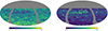 |
Fig. 5. Number counts (left) and median rms (right) for RACS in equatorial coordinates, in Nside = 32 HEALP IX maps, with no flux density cuts applied. |
The parameters for the simulated data set are estimated and shown in Table 3. The noise variation of the simulated catalogue is based on the Nside = 32 RACS rms map shown in Fig. 5, which in this case means that the rms map is a perfect representation of the noise in the catalogue. The rms estimator retrieves the injected dipole parameters, with a much higher significance than the standard Poisson estimator.
The results for RACS are shown in Table 3, showing a rather large discrepancy between the two pixel scales, and with respect to other results as well. In both cases, the dipole amplitude is increased with respect to the quadratic and basic Poisson estimators, and the direction is no longer agreeing with the direction of the CMB dipole. The Nside = 32 map seems to be less affected than the Nside = 64 map, but in both cases the dipole direction is further away from the CMB dipole direction, with Δθ ∼ 40° and Δθ ∼ 45° separation for the Nside = 32 and Nside = 64 maps, respectively. Especially striking is the recovered dipole direction of the Nside = 64 map, which is at a declination of −40 deg. This retrieved dipole direction aligns towards the anisotropy retrieved in the simulated data with the 1 mJy flux density threshold. Rather than pointing to an additional systematic effect that is not modelled by the local rms, it is therefore more likely that the median rms noise per cell does not adequately represent the noise variation observed in the catalogue.
To further investigate these results, the power-law fits to the cells are shown in Fig. 6, indicating that both power laws are a good fit to the distribution. For the Nside = 64 map, the relation fits less well to the cells with lower number counts, possibly indicating that the power-law assumption breaks down for these cells. One effect that can contribute to this is that, at such low number counts, the median rms will be a less robust measure of the local noise. As is the case for the other RACS results, there is a misalignment in right ascension that is even more pronounced here (see also Fig. 3). As seen in Fig. 4, the dipole amplitude is also increased. For the Nside = 32 map, the dipole amplitude is 3.8 times higher than the CMB expectation with a formal significance of 10σ, and for the Nside = 64 map the dipole amplitude is 4.7 times higher with a formal significance of 8σ.
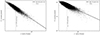 |
Fig. 6. Cell counts of the Nside = 32 (left) and Nside = 64 (right) HEALP IX maps with no flux density cuts applied, as a function of the median rms of the pixels, along with the best-fit power-law model (black solid line). The determined σ0 is indicated by the dashed vertical line; it intercepts the power law at the best-fit monopole value indicated by the horizontal dashed line. |
5.3. Combining RACS and NVSS
Following the procedure laid out in Sect. 3.4, we obtain a combined estimate of the dipole parameters of NVSS and RACS, assuming a common dipole amplitude but independent monopole amplitudes. Although we show that slightly different dipole amplitudes are to be expected between the catalogues, the degree of this difference depends entirely on the degree to which the inferred dipole is kinetic. Nevertheless, because of the nature of parameter estimation with MCMC, any differences in dipole amplitude between the catalogues will be absorbed into the overall uncertainty of the estimated parameters. In terms of monopole, there is no question as to the difference between the catalogues, as from the estimates of the individual catalogues –even with the same cut in flux density– there are large differences in source density.
Table 3 shows the results of the dipole parameters for the combined estimate of NVSS + RACS. Whereas the dipole directions for the individual catalogues were misaligned with the CMB dipole direction, the combined estimate favours a dipole direction that is perfectly aligned (Δθ = 4°, see Fig. 3) with that of the CMB dipole. In line with this finding, the dipole amplitude is reduced with respect to either of the individual catalogues; however, is still in tension with the CMB dipole. The dipole amplitude is three times higher than the CMB expectation, with a significance of 4.8σ for both the Nside = 32 and Nside = 64 maps. If we base our belief in a dipole result on its agreement with the CMB dipole in terms of direction, then this is the most significant and reliable result we obtain in this work. It is furthermore the most significant result obtained with radio sources to date, matching the significance of the dipole estimate with WISE AGN from Secrest et al. (2022), although less significant than the joint WISE+NVSS result from the same work.
6. Discussion
The results presented here demonstrate the potential of our introduced estimators and present at the very least an alternative method of making dipole measurements in present and future surveys. Figure 7 shows the results from this work compared to the most recent results from various surveys taken from Siewert et al. (2021) and Secrest et al. (2022) in terms of dipole amplitude. The NVSS is consistent across all works, as it is with our results. The results obtained here agree within uncertainties with those from Secrest et al. (2022), with the exception of RACS-rms and the WISE measurements. The same goes for the findings of Siewert et al. (2021), with the exception of the TGSS result. Though the extremely high amplitude of TGSS is attributed to a frequency dependence of the dipole in Siewert et al. (2021), the WISE result from Secrest et al. (2022) does not follow the fitted trend. Secrest et al. (2022) suggest that the TGSS result might deviate due to issues in flux calibration. As we have measurements at different frequencies, we can tentatively check whether results match up with the frequency evolution model of the dipole amplitude from Siewert et al. (2021), which predicts 𝒟 = 2.3 × 10⁻² at the RACS frequency of 887 MHz. Our RACS result for a flux cut of 15 mJy, which agrees with NVSS, does not follow the trend predicted by the model; however, the 150 mJy TGSS flux density cut made in Siewert et al. (2021) corresponds to a 40 mJy flux cut in RACS (assuming α = 0.75). Applying this flux density cut using the Nside = 32 RACS map, the inferred dipole direction shifts by Δθ = 8.8°, and the dipole amplitude increases to 𝒟 = (1.94 ± 0.37)×10−2. As such, our results cannot rule out the frequency dependence predicted by Siewert et al. (2021), but the obtained results from WISE AGN (Secrest et al. 2021, 2022; Dam et al. 2022) provide a strong argument against it. Though our results are consistent with the literature, as with many works concerning the dipole, their validity and that of the methods require further examination.
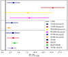 |
Fig. 7. Dipole amplitudes with 3σ uncertainties compared to the amplitude expected from the CMB from this work and to results from Siewert et al. (2021) and Secrest et al. (2022). The results from the different works are separated by horizontal dashed lines, showing the results from this work at the bottom. |
6.1. The Poisson solution
Though we show results here that are both internally consistent and consistent with other dipole estimates, the choice of a Poisson estimator might seem like an unnecessary constraint on the data; after all, the quadratic estimator shows an adequate performance and does not suffer any loss in precision compared to the Poisson estimator. Table 3 lists the χ2 values for the obtained results, defined by Eqs. (8) and (15) for the quadratic and Poisson estimators, respectively. As the quadratic estimator is minimised for a Gaussian distribution with mean equal to the variance, the quadratic and basic Poisson estimators are expected to provide similar values. This is indeed the case for the results in Table 3, both in the estimated parameters and χ2 values.
The value of the Poisson assumption becomes readily apparent when extending the parameter space, as we do when taking into account the rms power-law relation. The main feature of a Poisson distribution is that one parameter is necessary to describe it, λ, which is both the mean and variance of the distribution. This is a strict requirement on a distribution, allowing more freedom in other parameters which would otherwise be degenerate with the parameters of the distribution. This means that fitting the rms power law does not work with a quadratic estimator for example; indeed, this latter, though minimised by a distribution with mean equal to the variance, still allows for a wider Gaussian distribution. As seen in Fig. 8, the distribution of number counts without any flux density cut applied resembles a Gaussian distribution, which is much wider than a Poisson distribution with the same mean. However, the quadratic estimator does allow such a wide distribution, and therefore will not converge on a solution that transforms this distribution to a Poisson distribution. Herein lies the power of the Poisson estimator, which makes modelling and fitting of systematic effects in the data a viable alternative to cutting and masking data. Nevertheless, one drawback is that it is imposing a Poisson distribution on the data, which can lead to spurious results if improperly applied.
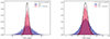 |
Fig. 8. Cell count distribution for Nside = 32 (left) and Nside = 64 (right) RACS maps without any flux density cuts applied. Raw counts are shown (blue histogram) alongside the counts corrected for the power-law fit (red histogram). A Poisson distribution with a λ equivalent to the estimated monopole amplitude is also shown (black histogram). |
Table 3 lists the χ2/d.o.f. values of the Poisson rms estimator after correction for the derived power law. The difference in distributions can be appreciated in Fig. 8, which shows the distributions of the cell counts of RACS without any flux density cut applied, along with the same distribution corrected for the rms power law that has been fit to the data. The uncorrected counts have a much wider distribution, which is clearly not Poisson, with χ2/d.o.f. = 13.28 for the Nside = 32 map and χ2/d.o.f. = 4.49 for the Nside = 64 map. The corrected counts resemble a Poisson distribution more closely, with χ2/d.o.f. = 2.03 for the Nside = 32 map and χ2/d.o.f. = 1.49 for the Nside = 64 map, but χ2/d.o.f. values indicate variance is still too large for a Poisson distribution, signifying that some residual effect has not been modelled by the estimator.
As such, the performance of the Poisson-rms estimator still leaves some questions to be answered. The assumption that source counts are related to sensitivity via a power law might carry a flaw, though there can be a number of possible reasons for this: (i) the median rms is not the best representation of the sensitivity of the survey in a given cell; (ii) the sensitivity only properly represents source counts down to some limit; and (iii) not all systematic effects equally impact source counts as well as sensitivity. These factors require further examination in the future, but remarkable already are the results when compared to the other RACS results. It is clear that this Poisson-rms estimator shows promise even in its basic form, and can be used as an additional test of the data for any survey that has information on the local rms. Furthermore, due to its flexibility, additional effects once characterised can easily be modelled and taken into account by the estimator.
6.2. Residual anisotropies in the data
In dipole measurements and other statistical studies that require large amounts of data to retrieve a statistically significant measure, it can be difficult to visually assess whether any one fit adequately describes the data. After all, we impose a model on the data to which the fit is restricted. For a rudimentary visual verification of whether or not the data follow the expected relations, we employ the hemisphere method used by Singal (2021). This method assumes that the direction of the dipole is already known, leaving the dipole amplitude as a function of angular distance from the dipole direction, 𝒟θ = 𝒟cos θ, as the only free parameter. To reach statistically significant number counts, the sky is divided into two hemispheres: hemisphere N1 with all sources between θ and θ + π/2, and hemisphere N2 with all sources between θ + π/2 and θ + π. The dipole amplitude as a function of θ is then written as
![$$ \begin{aligned} \mathcal{D} _{\theta } = \frac{N_1(\theta ) - N_2(\theta )}{\frac{1}{2}[N_1(\theta ) + N_2(\theta )]}\cdot \end{aligned} $$](/articles/aa/full_html/2023/07/aa46210-23/aa46210-23-eq27.gif)
We determine and plot the hemisphere results for NVSS and RACS assuming the results obtained from the Poisson estimators for the individual catalogues. The hemisphere relation for NVSS is presented in Fig. 9, which shows the data following the expected dipole curve except for the hemispheres closest to the dipole direction; these data reveal an increased anisotropy. This is more pronounced in the Nside = 64 map, where both θ = 0° and θ = 10° hemispheres show significantly increased counts compared to the expectation from the dipole model. In the Nside = 32 map, only the θ = 0° hemisphere shows increased counts, with all other points following the dipole model within uncertainties. This points to a residual anisotropy left in the data that has not influenced the overall fit.
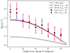 |
Fig. 9. Dipole amplitude of NVSS as a function of angular distance to the dipole direction, assuming a best-fit dipole direction from the basic Poisson estimator, for both Nside = 32 (blue) and Nside = 64 (red) maps. Alongside the data, the corresponding models are plotted (solid lines), as well as the expected model from the CMB dipole (black dashed line). |
For RACS, the hemisphere relations for both the basic Poisson estimator and the rms Poisson estimator are shown in Fig. 10. There is a residual anisotropy in RACS at 40° −60° from the dipole direction for both Nside = 32 and Nside = 64 maps that stands out immediately, especially in the results for the basic Poisson estimator. In the case of the basic Poisson estimator, as with NVSS, the fit is unaffected. However, this anisotropy might have had a significant impact on the rms Poisson estimator for the Nside = 64 map, as the dipole direction estimated from that map is 47° offset from the direction of the basic Poisson estimator, coinciding perfectly with the anisotropy seen at that angle. Indeed, the data for both Nside = 32 and Nside = 64 maps for the rms Poisson estimate agree well with the exception of the points closest to the dipole direction, which in the case of the Nside = 64 map are dominating the fit.
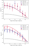 |
Fig. 10. Dipole amplitude of RACS as a function of angular distance to the dipole direction, assuming a best-fit dipole direction from the basic Poisson estimator (top) and Poisson rms estimator (bottom). Results for both Nside = 32 (blue) and Nside = 64 (red) maps are shown. Alongside the data, the corresponding models are plotted (solid lines), as well as the expected model from the CMB dipole (black dashed line). |
Finally, we investigate the possibility that residual systematic effects are present due to Galactic synchrotron. Secrest et al. (2022) use the de-striped and source-subtracted Haslam et al. (1982) 408 MHz all-sky map from Remazeilles et al. (2015) to mask pixels bright in Galactic synchrotron. To investigate if our results are impacted by Galactic synchrotron, we cross-correlate our number count maps with the Remazeilles et al. (2015) map. In all cases, no significant correlation is found (|ρ|< 0.05), showing that Galactic synchrotron is not present as a residual systematic effect in the data.
6.3. Combining and splitting catalogues
As shown in Sect. 5.3, combining catalogues as independent tracers of the dipole can provide a more robust measurement of the dipole, and in the case of NVSS and RACS, result in a dipole that matches the direction of the CMB dipole remarkably well, with a dipole amplitude of 2.5 times the CMB expectation. The justification for this approach is that radio data are a complex product and are sufficiently difficult to homogenise over a full survey internally, not to mention between surveys. Field of view, frequency, array configuration, calibration, imaging and source finding are all factors to consider when assessing the source counts in a given survey. For a key example of how these factors can influence source counts, we need to look no further than NVSS, which has been observed with two different array configurations at certain declination ranges. This is a systematic effect that produces different source densities depending on the configuration, something that can be plainly seen in the left plot of Fig. 1.
To demonstrate the potential of the Multi-Poisson estimator beyond combining independent catalogues, we repeated the dipole estimates for NVSS, lowering the minimum flux density in several steps. We then split the NVSS D and DnC configurations into separate catalogues, and repeated the experiment. The results are shown in Table 4 and Fig. 11, showing the effect of splitting the configuration on the dipole estimates. Immediately, we can see that, though the dipole estimate in both cases remains consistent in terms of right ascension, the separation of the catalogue produces wildly different results for flux density cuts below 15 mJy, both in terms of dipole amplitude and declination of the dipole direction. This result is expected to some degree, as the difference in source density between the D and DnC configurations is expected to produce an anisotropy in the north–south direction, which is largely alleviated (although not entirely) with the split in configurations. This is not only reflected in the declination of the dipole direction, but in the dipole amplitude as well, which is seen to decrease with more samples in the case of split configurations. Though the anisotropy in the declination is alleviated by this, another anisotropy in right ascension seems to start dominating at lower flux densities, dragging the dipole direction 43° from the CMB dipole direction.
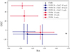 |
Fig. 11. Best-fit dipole directions with 1σ uncertainties for the complete NVSS (red) and split NVSS D + DnC (blue) catalogues, for lower flux density thresholds of 5, 10, and 15 mJy. The CMB dipole direction is indicated with a black star. |
Dipole estimates for NVSS using different flux density cuts, separating D and DnC configurations.
Though it seems that the different NVSS configurations produce an anisotropy that is on a similar level to other anisotropies related to incompleteness of the catalogue, and cannot therefore be reliably used to completely account for the systematic effects in the survey that appear when employing lower flux density thresholds, these results show that were such systematic effects to dominate the catalogue, restructuring the problem to consider these as multiple independent catalogues can produce sensible results. Our analysis is furthermore a useful test of the chosen flux density threshold, as for an appropriately chosen flux density threshold the results between the full catalogue and split catalogue should be consistent. The results here show that a flux density threshold of 15 mJy is indeed appropriate for the NVSS. Such an approach might become particularly relevant given that VLASS also uses different array configurations, which can be taken into account when estimating a dipole in the same manner as we have done for NVSS. Even for RACS, a prominent feature is a dependence of source counts on declination; though the exact mechanism is unclear, one possibility is related to the point spread function, as the UV-coverage of the array evolves with declination.
6.4. Combining catalogues and cosmological considerations
The combined dipole estimate of RACS and NVSS makes a compelling case for combining more probes of the cosmic dipole to increase sensitivity. The approach used here ostensibly carries less caveats than previous works, foregoing source matching, frequency scaling, subsampling, and weighting schemes, which can all introduce additional uncertainties. This carries with it a reduction in formal uncertainty, though there remain some factors regarding the nature of the dipole that can limit the approach. As the nature of the excess amplitude of the radio dipole is currently unknown, the approach of combining catalogues, even if done perfectly, carries an additional uncertainty. In Sect. 4, the expected kinematic dipole amplitudes for both NVSS and RACS are computed and are found to be nearly identical. This in large part justifies the obtention of a combined estimate of the catalogues; however, if we were to combine catalogues where the expected dipole amplitudes differed (e.g. when combining catalogues from multiple wavelengths), the approach would not be able to produce a reliable result without knowing the nature of the radio dipole. As it stands, we have a kinematic expectation of the radio dipole derived from the CMB. Given the velocity of the observer, this dipole is determined by the spectral index and flux distribution of the ensemble of sources. However, because of the measurement method used here, the excess dipole has an unknown origin, be it either kinetic or due to some entirely different effect.
Given the results obtained so far in this work and the literature, one could also assume an effect that somehow boosts the observed dipole with respect to the CMB dipole, or an additional anisotropy that is simply added to the kinematic dipole. Therefore, should we wish to combine for example the sample of WISE AGN, which has an expected dipole amplitude of 𝒟 = 7.3 × 10⁻³ (Secrest et al. 2022), with for example NVSS, a combined estimate would have to assume one of these models. Secrest et al. (2022) find that after removing the CMB dipole, assuming it is purely kinematic, the residual dipoles between NVSS and WISE agree with each other, favouring the interpretation of an intrinsic dipole anisotropy in the CMB rest frame. The results we obtain for NVSS and RACS also support this interpretation, the residual dipole amplitudes being 𝒟 = (0.97 ± 0.30)×10−2 and 𝒟 = (0.99 ± 0.24)×10−2, respectively. However, the expected dipoles of the catalogues are too similar to rule out other interpretations.
Furthermore, depending on which of the models presented above is the most accurate, survey design can have a profound impact on the measured cosmic radio dipole. The largest impact will be in the detected source populations and their redshift distributions. Naturally, going to optical or infrared wavelengths will yield different source populations that possibly trace the dipole differently, but even amongst radio surveys the detected source population will depend on the survey details. Radio surveys must be designed with a balance of depth and sky coverage, and so we imagine a scenario where the number of sources detected will stay constant over the survey due to this balance, leaving the significance of a dipole measurement unchanged. A shallow but large-sky-coverage radio survey will mostly detect AGN with a peaked redshift distribution, whereas a deep radio survey with limited sky coverage will probe most of the AGN population over all redshifts, as well as star-forming galaxies, which have a different redshift distribution from AGN altogether. Most surveys that have been used for dipole estimates fall into the first category, as proper coverage along the dipole axis is necessary. However, a survey falling into the second category would have the potential to differentiate between the possible models of the radio dipole we have laid out. The MeerKAT Absorption Line Survey (Gupta et al. 2016), consisting of sparsely spaced deep pointings homogeneously distributed across the sky, provides a good candidate for a survey falling into this second category, and therefore might provide more insight into the processes driving the anomalous amplitude of the radio dipole.
7. Conclusion
In this work, we present a set of novel Bayesian estimators for the purpose of measuring the cosmic radio dipole with the NVSS and RACS catalogues. Based on the assumption that counts-in-cell of radio sources follow a Poisson distribution, we construct estimators for the cosmic radio dipole based on Poisson statistics. To provide a means of for comparison, we include a quadratic estimator, which has been used in a number of previous dipole studies. We furthermore construct two extensions of the basic Poisson estimator to attempt to account for systematic effects in the respective catalogues. Firstly, we consider that if sensitivity information is present in the catalogue, this can be directly related to the local number density, assuming that systematic effects merely modify the local sensitivity of the catalogue. The local sensitivity and number counts are assumed to be related by a power law, the parameters of which can be estimated. We extend the Poisson estimator to address this. Secondly, we construct an extension to the Poisson estimator that can be given multiple separate catalogues –assuming that the catalogues trace the same dipole– and produces a combined estimate.
We obtain best-fit parameters for the cosmic radio dipole using χ2 minimisation for the quadratic estimator and using maximum likelihood estimation for the Poisson estimators. To discretise the sky, we use HEALP IX, producing maps with both Nside = 32 and Nside = 64. We verify that the quadratic estimator and basic Poisson estimator yield similar results, and that furthermore results between the pixel scales are consistent. We use the Poisson rms estimator on RACS while not using any cut in flux density to estimate the dipole parameters along with the parameters for the rms power law. The increased number counts greatly increase the precision of the estimate, but the results somewhat diverge from the dipole estimates produced by the basic estimators. Whether this difference is a genuine product of the data or a flaw in (assumptions of) the estimator is not perfectly understood, but the initial results are still promising given that the entire catalogue of sources is used. We finally use a Poisson estimator for multiple catalogues on NVSS and RACS and obtain a dipole estimate that perfectly aligns with the CMB dipole in terms of direction, but has an amplitude that is three times as large with a significance of 4.8σ. Given the dipole estimates obtained from the individual catalogues, this result is in line with expectations for a combination of the two catalogues, and can therefore be seen as the most reliable and significant result obtained here.
We explore the possibility of splitting up a catalogue and using the Poisson estimator for multiple catalogues to estimate the dipole as if on two independent catalogues. We use this method on the NVSS, which has been observed with two different array configurations, introducing an artifical north–south anisotropy in the catalogue. We treat these array configurations as separate catalogues and repeat the dipole estimate, and go down to lower flux density limits than with the basic Poisson estimator. We see that while using the whole NVSS, a north–south anisotropy starts to dominate the estimate at lower flux densities; separating the configuration largely mitigates this effect. As a result, this allows us to lower the flux density cut, increasing number counts and thus increasing the significance of the dipole estimates. This approach may work well on catalogues such as VLASS, which also uses different array configurations in different parts of the sky. The presented estimator may provide the potential to combine a larger variety of catalogues, but the extent to which this can be done depends in large part on the nature of the excess dipole. With an increasing array of probes at various wavelengths, sky coverage, and depth, reaching the necessary sensitivity to detect the dipole, the nature of this dipole may well soon be discovered, given the different populations of sources that can be probed.
Peebles (1980) uses this measure as a clustering statistic of the large-scale structure, and specifically to define the number of objects per cluster.
Acknowledgments
We thank the anonymous referee for their useful comments and feedback on the text. J.D.W. acknowledges the support from the International Max Planck Research School (IMPRS) for Astronomy and Astrophysics at the Universities of Bonn and Cologne. Some of the results in this paper have been derived using the healpy (Zonca et al. 2019) and HEALP IX (Górski et al. 2005) packages. This research has made use of TOPCAT (Taylor 2005), LMFIT (Newville et al. 2016), BILBY (Ashton et al. 2019), and EMCEE (Foreman-Mackey et al. 2013).
References
- Aghanim, N., Akrami, Y., Arroja, F., et al. 2020, A&A, 641, A1 [NASA ADS] [CrossRef] [EDP Sciences] [Google Scholar]
- Ashton, G., Hübner, M., Lasky, P. D., et al. 2019, ApJS, 241, 27 [NASA ADS] [CrossRef] [Google Scholar]
- Blake, C., & Wall, J. 2002, Nature, 416, 150 [NASA ADS] [CrossRef] [Google Scholar]
- Böhme, L., Schwarz, D. J., de Gasperin, F., Röttgering, H. J. A., & Williams, W. L. 2023, A&A, 674, A189 [NASA ADS] [CrossRef] [EDP Sciences] [Google Scholar]
- Colin, J., Mohayaee, R., Rameez, M., & Sarkar, S. 2017, MNRAS, 471, 1045 [Google Scholar]
- Condon, J. J. 1992, ARA&A, 30, 575 [Google Scholar]
- Condon, J. J., & Ransom, S. M. 2016, Essential Radio Astronomy (Princeton: Princeton University Press) [Google Scholar]
- Condon, J. J., Cotton, W. D., Greisen, E. W., et al. 1998, AJ, 115, 1693 [Google Scholar]
- Dalang, C., & Bonvin, C. 2022, MNRAS, 512, 3895 [NASA ADS] [CrossRef] [Google Scholar]
- Dam, L., Lewis, G. F., & Brewer, B. J. 2022, ArXiv e-prints [arXiv:2212.07733] [Google Scholar]
- Darling, J. 2022, ApJ, 931, L14 [NASA ADS] [CrossRef] [Google Scholar]
- Ellis, G. F. R., & Baldwin, J. E. 1984, MNRAS, 206, 377 [NASA ADS] [CrossRef] [Google Scholar]
- Foreman-Mackey, D., Hogg, D. W., Lang, D., & Goodman, J. 2013, PASP, 125, 306 [Google Scholar]
- Górski, K. M., Hivon, E., Banday, A. J., et al. 2005, ApJ, 622, 759 [Google Scholar]
- Guandalin, C., Piat, J., Clarkson, C., & Maartens, R. 2022, ArXiv e-prints [arXiv:2212.04925] [Google Scholar]
- Gupta, N., Srianand, R., Baan, W., et al. 2016, Proceedings of MeerKAT Science: On the Pathway to the SKA, 25–27 May, 2016 Stellenbosch, South Africa (MeerKAT2016), 14 [Google Scholar]
- Hale, C. L., McConnell, D., Thomson, A. J. M., et al. 2021, PASA, 38, e058 [NASA ADS] [CrossRef] [Google Scholar]
- Haslam, C. G. T., Salter, C. J., Stoffel, H., & Wilson, W. E. 1982, A&AS, 47, 1 [NASA ADS] [Google Scholar]
- Intema, H. T., Jagannathan, P., Mooley, K. P., & Frail, D. A. 2017, A&A, 598, A78 [NASA ADS] [CrossRef] [EDP Sciences] [Google Scholar]
- Lacy, M., Baum, S. A., Chandler, C. J., et al. 2020, PASP, 132, 035001 [Google Scholar]
- Mauch, T., Murphy, T., Buttery, H. J., et al. 2003, MNRAS, 342, 1117 [Google Scholar]
- McConnell, D., Hale, C. L., Lenc, E., et al. 2020, PASA, 37, e048 [Google Scholar]
- Mohan, N., & Rafferty, D. 2015, Astrophysics Source Code Library [record ascl:1502.007] [Google Scholar]
- Newville, M., Stensitzki, T., Allen, D. B., et al. 2016, Astrophysics Source Code Library [record ascl:1606.014] [Google Scholar]
- Peebles, P. J. E. 1980, The Large-Scale Structure of the Universe (Princeton: Princeton University Press) [Google Scholar]
- Remazeilles, M., Dickinson, C., Banday, A. J., Bigot-Sazy, M.-A., & Ghosh, T. 2015, MNRAS, 451, 4311 [Google Scholar]
- Rengelink, R. B., Tang, Y., de Bruyn, A. G., et al. 1997, A&AS, 124, 259 [NASA ADS] [CrossRef] [EDP Sciences] [Google Scholar]
- Rubart, M., & Schwarz, D. J. 2013, A&A, 555, A117 [NASA ADS] [CrossRef] [EDP Sciences] [Google Scholar]
- Secrest, N. J., von Hausegger, S., Rameez, M., et al. 2021, ApJ, 908, L51 [Google Scholar]
- Secrest, N. J., von Hausegger, S., Rameez, M., Mohayaee, R., & Sarkar, S. 2022, ApJ, 937, L31 [NASA ADS] [CrossRef] [Google Scholar]
- Shimwell, T. W., Tasse, C., Hardcastle, M. J., et al. 2019, A&A, 622, A1 [NASA ADS] [CrossRef] [EDP Sciences] [Google Scholar]
- Siewert, T. M., Hale, C., Bhardwaj, N., et al. 2020, A&A, 643, A100 [EDP Sciences] [Google Scholar]
- Siewert, T. M., Schmidt-Rubart, M., & Schwarz, D. J. 2021, A&A, 653, A9 [NASA ADS] [CrossRef] [EDP Sciences] [Google Scholar]
- Singal, A. K. 2011, ApJ, 742, L23 [NASA ADS] [CrossRef] [Google Scholar]
- Singal, A. K. 2021, Universe, 7, 107 [NASA ADS] [CrossRef] [Google Scholar]
- Taylor, M. B. 2005, ASP Conf. Ser., 347, 29 [Google Scholar]
- Wagenveld, J. 2023, https://doi.org/10.5281/zenodo.7962923 [Google Scholar]
- Wagenveld, J. D., Klöckner, H.-R., Gupta, N., et al. 2023, A&A, 673, A113 [NASA ADS] [CrossRef] [EDP Sciences] [Google Scholar]
- Wright, E. L., Eisenhardt, P. R., Mainzer, A. K., et al. 2010, AJ, 140, 1868 [Google Scholar]
- Zonca, A., Singer, L. P., Lenz, D., et al. 2019, J. Open Source Softw., 4, 1298 [NASA ADS] [CrossRef] [Google Scholar]
All Tables
Dipole estimates using the various estimators on the NVSS and RACS catalogues, including a combined estimate using both catalogues.
Dipole estimates for NVSS using different flux density cuts, separating D and DnC configurations.
All Figures
|
Fig. 1. Source density of NVSS (left) and RACS (right) as a function of declination for different flux density cuts. For the NVSS, we show the boundaries where different array configurations are used. In both cases, the catalogues can be seen to be inhomogeneous at low flux densities. |
| In the text | |
|
Fig. 2. Number counts for NVSS (left) and RACS (right) in equatorial coordinates, in Nside = 32 HEALP IX maps with masks and a flux density cut of 15 mJy applied. |
| In the text | |
|
Fig. 3. Best-fit dipole directions for the Poisson estimator of NVSS (blue), RACS (red), RACS with rms power law (green), and NVSS+RACS (purple) compared with the CMB dipole direction (black star). Different transparency levels represent 1σ, 2σ, and 3σ uncertainties. In all cases, results from the Nside = 32 HEALPix map are shown. |
| In the text | |
|
Fig. 4. Best-fit dipole amplitudes with 3σ uncertainties for the Poisson estimator of NVSS (blue), RACS (red), RACS with rms power law (green), and NVSS+RACS (purple), compared with an expected CMB dipole amplitude of 𝒟 = 4.5 × 10⁻³ (black line). Both results from the Nside = 32 and Nside = 64 HEALP IX maps are shown. |
| In the text | |
|
Fig. 5. Number counts (left) and median rms (right) for RACS in equatorial coordinates, in Nside = 32 HEALP IX maps, with no flux density cuts applied. |
| In the text | |
|
Fig. 6. Cell counts of the Nside = 32 (left) and Nside = 64 (right) HEALP IX maps with no flux density cuts applied, as a function of the median rms of the pixels, along with the best-fit power-law model (black solid line). The determined σ0 is indicated by the dashed vertical line; it intercepts the power law at the best-fit monopole value indicated by the horizontal dashed line. |
| In the text | |
|
Fig. 7. Dipole amplitudes with 3σ uncertainties compared to the amplitude expected from the CMB from this work and to results from Siewert et al. (2021) and Secrest et al. (2022). The results from the different works are separated by horizontal dashed lines, showing the results from this work at the bottom. |
| In the text | |
|
Fig. 8. Cell count distribution for Nside = 32 (left) and Nside = 64 (right) RACS maps without any flux density cuts applied. Raw counts are shown (blue histogram) alongside the counts corrected for the power-law fit (red histogram). A Poisson distribution with a λ equivalent to the estimated monopole amplitude is also shown (black histogram). |
| In the text | |
|
Fig. 9. Dipole amplitude of NVSS as a function of angular distance to the dipole direction, assuming a best-fit dipole direction from the basic Poisson estimator, for both Nside = 32 (blue) and Nside = 64 (red) maps. Alongside the data, the corresponding models are plotted (solid lines), as well as the expected model from the CMB dipole (black dashed line). |
| In the text | |
|
Fig. 10. Dipole amplitude of RACS as a function of angular distance to the dipole direction, assuming a best-fit dipole direction from the basic Poisson estimator (top) and Poisson rms estimator (bottom). Results for both Nside = 32 (blue) and Nside = 64 (red) maps are shown. Alongside the data, the corresponding models are plotted (solid lines), as well as the expected model from the CMB dipole (black dashed line). |
| In the text | |
|
Fig. 11. Best-fit dipole directions with 1σ uncertainties for the complete NVSS (red) and split NVSS D + DnC (blue) catalogues, for lower flux density thresholds of 5, 10, and 15 mJy. The CMB dipole direction is indicated with a black star. |
| In the text | |
Current usage metrics show cumulative count of Article Views (full-text article views including HTML views, PDF and ePub downloads, according to the available data) and Abstracts Views on Vision4Press platform.
Data correspond to usage on the plateform after 2015. The current usage metrics is available 48-96 hours after online publication and is updated daily on week days.
Initial download of the metrics may take a while.