| Issue |
A&A
Volume 697, May 2025
|
|
|---|---|---|
| Article Number | A112 | |
| Number of page(s) | 11 | |
| Section | Cosmology (including clusters of galaxies) | |
| DOI | https://doi.org/10.1051/0004-6361/202453397 | |
| Published online | 12 May 2025 | |
The kinematic contribution to the cosmic number count dipole
1
Max-Planck Institut fur Radioastronomie, Auf dem Hügel 69, 53121 Bonn, Germany
2
Department of Physics, University of Oxford, Parks Road, Oxford OX1 3PU, UK
3
Fakultät für Physik, Universität Bielefeld, Postfach 100131, 33501 Bielefeld, Germany
⋆ Corresponding author.
Received:
11
December
2024
Accepted:
1
March
2025
Abstract
Measurements of the number-count dipole with large surveys have shown amplitudes in tension with kinematic predictions based on the observed Doppler dipole of the cosmic microwave background (CMB). These observations seem to be in direct conflict with a homogeneous and isotropic universe as asserted by the cosmological principle, demanding further investigation into the origin of the tension. Here, we investigated whether the observed number-count dipoles are consistent with being fully kinematic, regardless of boost, or if there is any residual anisotropy contributing to the total observed dipole, independent of the kinematic part. To disentangle these contributions, we aim to leverage the fact that the kinematic matter dipole expected in a given galaxy catalogue scales with observed properties of the sample, and different catalogues used in the literature therefore have different kinematic dipole expectations. We performed joint dipole fits using the NRAO VLA Sky Survey (NVSS), the Rapid ASKAP Continuum Survey (RACS), and the active galactic nuclei (AGN) catalogue derived from the Wide-field Infrared Survey Explorer (CatWISE). The direction of the common dipole between these catalogues is offset from the CMB dipole direction by 23 ± 5 degrees. Assuming a common kinematic and non-kinematic dipole component between all catalogues, we find that a large residual, non-kinematic dipole anisotropy is detected, though a common direction between the two components is disfavoured by model selection. Freeing up both amplitude and direction for this residual dipole while fixing the kinematic dipole to the CMB dipole expectation, we recover a significant residual dipole with 𝒟resid = (0.81 ± 0.14)×10−2, which is offset from the CMB dipole direction by 39 ± 8 degrees. While these results cannot explain the origin of the unexpectedly large number-count dipoles, they offer a rephrasing of the anomaly in terms of kinematic and non-kinematic contributions, providing evidence for the existence of the latter within the models explored here. The present work provides a valuable first test of this concept, although its scrutinising power is limited by the currently employed catalogues. Larger catalogues, especially in radio, will be needed to further lift the degeneracy between the kinematic and residual dipole components.
Key words: galaxies: statistics / cosmology: observations / large-scale structure of Universe
© The Authors 2025
 Open Access article, published by EDP Sciences, under the terms of the Creative Commons Attribution License (https://creativecommons.org/licenses/by/4.0), which permits unrestricted use, distribution, and reproduction in any medium, provided the original work is properly cited.
This article is published in open access under the Subscribe to Open model.
Open Access funding provided by Max Planck Society.
1. Introduction
Modern cosmological models based on Friedmann-Lemaître-Robertson-Walker (FLRW) metrics, such as Λ-CDM, are built on the assumptions of the cosmological principle. As such, these models require homogeneity and isotropy on the largest scales. While the cosmic microwave background (CMB) is a remarkable example of this large scale isotropy, with fluctuations around the CMB monopole being as small as one part in 105, the CMB dipole appears to be an exception. A hundred times larger than the smaller scale fluctuations, the CMB dipole is conventionally considered to be the result of our movement with respect to the frame in which the CMB would have appeared isotropic, the so-called CMB rest frame. Under this interpretation, measurements of the CMB dipole translate a velocity of the Solar System with respect to the CMB of v = 369.82 ± 0.11 km s−1 (Planck Collaboration I 2020).
Our movement is also expected to result in an apparent dipole in the number counts of cosmologically distant sources, whose rest frame should agree with that of the CMB (Ellis & Baldwin 1984). Caused by the relativistic effects of aberration, Doppler boosting, and Doppler shifting of the observed source positions and spectra, the same physics is at play as that suspected at the root of the CMB dipole. This immediately places an expectation on the kinematic matter dipole: a dipole pointing in the same direction as the CMB dipole with an amplitude proportional to β = v/c, where c is the speed of light. To measure the expected 𝒪(10−3) number-count dipole, it was predicted that catalogues of extragalactic sources in excess of 106 were required to reach 3σ statistical significance (Crawford 2009). The earliest statistically significant measurements were performed with a catalogue of radio sources from the National Radio Astronomy Observatory (NRAO) Very Large Array (VLA) Sky Survey (NVSS, Condon et al. 1998), where the measured dipole consistently had a larger amplitude than expected (e.g. Blake & Wall 2002; Singal 2011; Rubart & Schwarz 2013; Siewert et al. 2021; Secrest et al. 2022; Wagenveld et al. 2023), while being broadly consistent with the CMB dipole in terms of direction. Other radio catalogues have since been used for this measurement with varying levels of success, yielding similar results; however, without independent measurements at other wavelengths it was difficult to exclude common systematic effects as the cause of the dipole.
An important breakthrough in the credibility of these measurements was the recent addition of a measurement of the number-count dipole with infrared active galactic nuclei (AGN, Secrest et al. 2021, 2022; Dam et al. 2023). This measurement was performed with a catalogue of sources observed by the Wide-field Infrared Survey Explorer (WISE, Wright et al. 2010). As WISE is a space-based telescope, it is not influenced by any of the potential systematic effects that would affect ground-based radio observations. Furthermore, the sample of sources was entirely independent of NVSS and other radio catalogues. This measurement yielded a dipole amplitude that was two times larger than the kinematic expectation, with a significance level of 4.9σ. As a consequence, these measurements are in serious tension with the cosmological principle. Since this measurement with infrared AGN, additional measurements of the dipole with quasars selected in a composition of optical and infrared measurements (Mittal et al. 2024b,a) have also shown a higher amplitude than expected, although to a less significant degree; this is due to lower source counts. An excess dipole has now been confirmed at different wavelengths, with different instruments, and in different independent source samples.
With such pronounced excess dipoles measured in these catalogues, the question arises as to whether the measured dipole is purely caused by the velocity of the observer, as is assumed in Ellis & Baldwin (1984). Rather than a purely kinematic “Ellis & Baldwin dipole”, some other (residual) component could be contributing to the total observed dipole, that does not scale with β. Such a question lies at the core of studies employing a range of methods to scrutinise the kinematic dipole signals detected (and suspected) thus far. For instance, the CMB Doppler dipole is expected to be accompanied by aberration of the CMB anisotropies, and though corresponding measurements indeed report consistency (Planck Collaboration XXVII 2014; Saha et al. 2021; Ferreira & Quartin 2021), it has not been conclusively shown that the CMB dipole is entirely kinematic. For the number-count dipole, methods to measure kinematic and non-kinematic components separately have been proposed (e.g. Nadolny et al. 2021; Tiwari et al. 2015), although these require a great deal more data than what is currently available. Only recently, Ferreira & Marra (2024) and Tiwari et al. (2024) attempted to measure the kinematic dipole directly using redshifts from the Sloan Digital Sky Survey (SDSS). While there is an indication for consistency with the CMB dipole, large uncertainties remain. Separate measures of the Solar System velocity, for example with SNIa (e.g. Horstmann et al. 2022), seem to be consistent with the velocity obtained from the CMB dipole as well. However, an explicit separation of kinematic and non-kinematic dipoles has not been made, and these components have so far not been independently and simultaneously measured.
We here implement an alternative method for isolating the kinematic dipole, as expected from Ellis & Baldwin (1984), from a potential non-kinematic residual dipole, by using multiple catalogues at the same time. We aim to achieve this by utilising the dipole estimator from Wagenveld et al. (2023), which is able to fit a common dipole signal from a set of catalogues. This avoids the problems that stem from attempting to combine the catalogues due to differences in frequency, angular resolution, and flux density limit (e.g. Colin et al. 2017; Darling 2022). Previously, this procedure has allowed a combined dipole estimate of NVSS and the Rapid Australian Square Kilometre Array Pathfinder (ASKAP) Continuum Survey (RACS-low, Hale et al. 2021). This measurement was possible because the predicted (kinematic) dipole amplitude of both catalogues was the same. While true for the case of NVSS, RACS-low, and other radio catalogues, this is not the case in general. For instance, for CatWISE the expected dipole amplitude is nearly twice that of NVSS and RACS-low. Under certain assumptions, chief of which is that any residual non-kinematic dipole component is common between the catalogues, using catalogues with different expected kinematic dipole amplitudes allows a combined estimate to be used to separate these components.
In this work, we use the NVSS, RACS-low and CatWISE AGN catalogues and their different expected kinematic dipole amplitudes to isolate the kinematic component of the number-count dipole. The paper is organised as follows. In Sect. 2 we describe the estimators, and in Sect. 3 we describe the data we used to perform this measurement. The results are presented in Sect. 4 and discussed in Sect. 5. We conclude in Sect. 6.
2. The cosmic number-count dipole
As a result of Doppler boost, Doppler shift, and relativistic aberration induced by our velocity with respect to background sources, we see a dipole in the observed number counts of extragalactic background sources. The amplitude of this kinematic number-count dipole, caused by the velocity of the observer β = v/c, is given by (Ellis & Baldwin 1984)
![Mathematical equation: $$ \begin{aligned} \mathcal{D} _{kin} = [2 + x(1+\alpha )]\beta \end{aligned} $$](/articles/aa/full_html/2025/05/aa53397-24/aa53397-24-eq1.gif) (1)
(1)
and depends on the spectral index of the sources, α1, and the power-law index of the flux density distribution, x. These parameters in general differ per catalogue and survey, and as such the expected kinematic dipole amplitude for a given β can also differ. Given the fact that the measured dipole amplitude has in many cases been larger than the expected kinematic dipole amplitude, the possibility arises that the excess dipole amplitude is not kinematic, but is caused by a different phenomenon altogether. In this case (assuming that both components point in the same direction), we can hypothesise that the total dipole amplitude can be broken down as
 (2)
(2)
where 𝒟kin is the Ellis & Baldwin (1984) prediction from Eq. (1), and 𝒟resid represents the contribution of a residual, non-kinematic dipole component. While the fact that the total dipole we measure is relatively close to the CMB dipole in terms of direction indicates that any residual dipole might also point in a similar direction, it is unlikely that the separate components point in the exact same direction. We distinguish corresponding considerations following Eq. (8).
2.1. Dipole estimation
For dipole estimation, we expanded upon the existing Bayesian estimators introduced in Wagenveld et al. (2023). These estimators are based on the fact that the counts-in-cells distribution of sources isotropically distributed across the sky follows a Poisson distribution:
 (3)
(3)
where n is the number of sources in a cell and λ represents the mean and variance of the distribution. The most basic Poisson estimator assumes only a dipole and monopole, which affect λ as
 (4)
(4)
Here, ℳ represents the monopole, and d represents the dipole vector, the amplitude of which is 𝒟. In order to estimate the dipole parameters, we maximise the likelihood given by
 (5)
(5)
over all cells i. In Wagenveld et al. (2023), this likelihood was found to produce similar results to quadratic estimators and outperforms them in the limit of low, counts where the assumption of Gaussian noise no longer holds. It was also shown that this basic estimator can be extended in several ways to increase the number of usable sources for a dipole measurement while accounting for systematics. One such extension of the basic Poisson estimator was used in Wagenveld et al. (2024) to fit an additional linear relation between a specific parameter y and the source density
, \end{aligned} $$](/articles/aa/full_html/2025/05/aa53397-24/aa53397-24-eq6.gif) (6)
(6)
where ε is defined as the slope of the linear relation. Below, we use this estimator to fit the observed change in source density as a function of absolute ecliptic latitude seen in CatWISE (Secrest et al. 2021), similarly to what was done in Dam et al. (2023). As demonstrated in Dam et al. (2023), not including the ecliptic latitude effect is heavily disfavoured by model selection and yields an even higher dipole amplitude than if it is included.
2.2. Joint-dipole estimation
Another extension of the basic Poisson estimator is the multi-Poisson estimator, which can incorporate multiple catalogues and perform a joint-dipole estimation. This estimator assumes a common dipole but a different monopole for each catalogue, thereby allowing the fitting of a common dipole signal. The likelihood of this estimator is defined as
![Mathematical equation: $$ \begin{aligned} \mathcal{L} (\boldsymbol{n}|\boldsymbol{d},\boldsymbol{\mathcal{M} }) = \prod _j \left[\prod _i \frac{\lambda (\mathcal{M} _j,\boldsymbol{d})^{n_{i,j}}e^{-\lambda (\mathcal{M} _j,\boldsymbol{d})}}{n_{i,j}!}\right], \end{aligned} $$](/articles/aa/full_html/2025/05/aa53397-24/aa53397-24-eq7.gif) (7)
(7)
taking the product over each cell, i, in each catalogue, j, and taking the product of all catalogues. The efficacy of this estimator is, however, predicated on the fact that the catalogues have the same dipole signal, whereas the amplitude of the kinematic dipole actually depends on the spectral indices and flux density distribution of the sources in the catalogue. As such, if we wish to combine catalogues with different expected kinematic dipole amplitudes, this presents an opportunity to (under certain assumptions) actually isolate the kinematic dipole from any other components contributing to the dipole, following Eq. (2). Based on this principle, we redefine the dipole vector d in Eq. (7) as
![Mathematical equation: $$ \begin{aligned} \boldsymbol{d}_j = [2 + x_j(1+\alpha _j)]\boldsymbol{\beta } + \boldsymbol{d}_{resid} \end{aligned} $$](/articles/aa/full_html/2025/05/aa53397-24/aa53397-24-eq8.gif) (8)
(8)
for catalogue j, where each catalogue has a different pair of x and α values. To achieve a better understanding of which model describes the data the best, we considered the different hypotheses listed below.
(0) The dipole consists of a single component, which is fully kinematic.
(i) The dipole consists of two components, one kinematic and one residual, which both point in the same direction.
(ii) The dipole consists of two components, one kinematic and one residual, which both point in different directions.
(iii) The dipole consists of two components, one kinematic and one residual, which both point in different directions. The kinematic component is fixed to what is expected from the CMB dipole in both amplitude and direction.
Here, hypothesis (0) is considered our ‘null’ hypothesis and seeks to explain the observed dipole purely by kinematics. In all other cases, we separate the kinematic contribution and residual dipole, described by β and dresid, respectively. If the direction of these components is the same, Eq. (8) simply becomes a linear equation with two unknowns, and it thus requires at least two measurements with significantly different outcomes to resolve. This is of course more complicated once we associate uncertainties with these measurements. In the two latter cases, we also allowed for separate directions for these two components. We stress here that the separation of dipole components as presented here assumes that different catalogues have the same dresid, even though the origin of this dipole component is not known. The validity of this assumption is discussed in Sect. 5.
2.3. Priors
To avoid biasing results, we aim to make priors as uninformed as possible. For the dipole, we fitted the right ascension and declination of the dipole direction, as well as the dipole amplitude, separately. We did not restrict or fix any particular direction (unless explicitly mentioned), so the priors on right ascension and declination of the dipole direction are the same for both the kinematic and residual dipoles. For individual catalogues, we were only able to fit for the total dipole amplitude 𝒟, while in the multi-Poisson estimator, we fitted for both β and 𝒟resid. We defined these priors such that the total dipole amplitude cannot exceed unity. Regardless of the estimator, we estimate the monopole ℳ for each catalogue separately, using the mean of all cell counts,  , as an initial estimate. We can summarise these general priors as follows:
![Mathematical equation: $$ \begin{aligned} \pi (\mathcal{D} )&\sim u \\ \pi (\mathcal{D} _{resid})&\sim 0.5\cdot u \\ \pi (\beta )&\sim 0.05\cdot u \\ \pi (\mathrm{RA} )&\sim 360\cdot u \\ \pi (\mathrm{Dec} )&\sim \sin ^{-1}[2u-1] \\ \pi (\mathcal{M} )&\sim 2\bar{n}\cdot u. \end{aligned} $$](/articles/aa/full_html/2025/05/aa53397-24/aa53397-24-eq10.gif)
Here, u = 𝒰[0, 1] represents a uniform distribution between 0 and 1. For the Poisson estimator implementing a linear fit described in Eq. (6), we fitted for an additional parameter ε. The only requirement for this parameter is that the resulting number counts should not be negative, making the prior dependent on the maximum value of y, such that π(ε)∼(2u − 1)/ymax.
All above-described estimators were implemented using the Bayesian inference library BILBY (Ashton et al. 2019). Through BILBY, we maximised the likelihood with MCMC sampling using EMCEE (Foreman-Mackey et al. 2013). After sampling, the best-fit parameters were obtained by taking the median of the posterior distribution, with the uncertainties represented by the 16% (lower) and 84% (upper) quantiles of the distribution. The scripts in which these were implemented are available on GitHub2, and an immutable copy is archived in Zenodo (Wagenveld 2025). For the purposes of model comparison, we used HARMONIC, which implements the learnt harmonic mean estimator (McEwen et al. 2021) to compute the marginal likelihood, 𝒵.
3. Data
For the purposes of testing these hypotheses, we combined several catalogues that have different expected kinematic dipole amplitudes. These catalogues should also provide reliable dipole measurements on their own, and thus be large enough to yield a significant dipole measurement individually. Furthermore, for combined measurements, we want to select catalogues that can easily be made statistically independent from each other. In a purely kinematic interpretation of the number-count dipole, the dipole signal is dominated by sources near the flux density limit. As such, covering an completely independent sample of sources is not necessary for a statistically independent measurement. If, however, an intrinsic dipole is thought to contribute to the overall dipole, then this signal can originate from the overall observed source population. This motivates the use of the RACS-low, NVSS, and CatWISE catalogues, which all have independently yielded robust and significant measurements of the number-count dipole. With NVSS and RACS-low covering the northern and southern hemisphere radio populations, respectively, and CatWISE covering the infrared quasar population, these catalogues mostly see different sources. As such, they are easily made completely statistically independent by removing shared sources, enabling joint dipole measurements to constrain the contribution of a residual dipole effect.
For all catalogues, in order to predict the kinematic dipole amplitude, we must determine the index of the power law, x, describing the integral flux density distribution of sources, and the (average) spectral index of sources, α. Because the dipole effect is dominated by sources near the lower flux density limit, these values should be measured in the vicinity of this limit (von Hausegger 2024). In all cases, these values are determined after the final data cuts described in Sect. 3.4. We note that as we are only determining the values here, they are not included as free parameters in the dipole estimation, as they would add a significant number of additional nuisance parameters. As such, though these values can be noisy, their variance is not included in the modelling, which can in principle lead to an underestimation of the overall uncertainty in the other (dipole) parameters. However, we expect this variance to be highly suppressed given the fact that they are measured for the entire catalogue (as seen in Secrest et al. 2022).
3.1. NVSS
The NVSS catalogue (Condon et al. 1998) was the first catalogue on which a significant dipole measurement could be performed (Blake & Wall 2002) and was also the first catalogue for which an excess dipole amplitude was claimed (Singal 2011). It covers the entire sky north of a declination of −40° at a frequency of 1.4 GHz and an angular resolution of 45″. The full catalogue, which includes the Galactic plane, contains 1 773 484 sources. To homogenise the catalogue for a dipole measurement, we made a flux density cut at 15 mJy. The flux density distribution around this cut is well fitted by a power law with an index of x = 0.74. While no spectral indices are available for NVSS, at a frequency of 1.4 GHz the mean spectral index is commonly found to be around 0.75 (e.g. Condon 1984). As such, we adopted α = 0.75 for NVSS, which sets the expectation for a purely kinematic dipole with a canonical velocity of β = 1.23 × 10⁻³ to 𝒟 = 0.41 × 10⁻².
3.2. RACS-low
The RACS project (McConnell et al. 2020) covers the sky south of a declination of +30° and is being released in several stages at different frequencies. The first of these data releases is RACS-low, which was first used for a dipole measurement in conjunction with the VLA Sky Survey (VLASS, Lacy et al. 2020) by Darling (2022); however, the first dipole measurement with only RACS-low was performed by Wagenveld et al. (2023). RACS-low has an angular resolution of 25″ and a central frequency of 887.5 MHz. The RACS-low catalogue, which does not include the Galactic plane, contains 2 123 638 sources. To homogenise the catalogue for a dipole measurement, we made the same flux density cut as for NVSS at 15 mJy. The flux density distribution around this cut is well fitted by a power law with an index of x = 0.72. flux density comparisons of RACS-low, NVSS, and RACS-mid indicate steeper spectral indices for these sources (Hale et al. 2021; Duchesne et al. 2023), as the lower frequency observations will detect more sources with steeper spectra. Thus, for RACS-low, we adopted α = 0.88 (the median α found in Duchesne et al. 2023), which translates to a kinematic dipole amplitude of 𝒟 = 0.41 × 10⁻² for our canonical velocity; this is identical to the expectation for NVSS.
3.3. CatWISE
The WISE telescope (Wright et al. 2010) is an infrared space-based telescope that has observed the whole sky. For a dipole measurement at infrared wavelengths, extragalactic sources must be reliably selected from the observations, which also contain stars and dusty galaxies. The CatWISE2020 catalogue, which contains more than a billion sources, is the largest and most recent catalogue compiled from these observations (Marocco et al. 2021). The AGN selected from this catalogue were used for the dipole measurement in Secrest et al. (2021), with an updated version of the catalogue, which we used here, being used for the dipole measurement in Secrest et al. (2022). In this present catalogue, AGN are selected with a W1 − W2 ≥ 0.8 cut, which leaves 4 145 046 sources in the catalogue, including the Galactic plane. To homogenise the catalogue, a cut of W1 < 16.5 was made, which corresponds to a flux density cut of 0.078 mJy. The flux density distribution of this WISE catalogue around this flux density cut is well fitted by a power law with an index of x = 1.90. Spectral indices are available for all the CatWISE sources; however, they do not follow a Gaussian distribution. Furthermore, spectral indices are generally lower for sources with lower flux densities. For sources below 0.08 mJy, the mean spectral index is α = 1.07, so that is the value we used for the WISE catalogue. Here, a purely kinematic dipole with the canonical velocity would have an amplitude of 𝒟 = 0.73 × 10⁻².
3.4. Masking and pixelisation
Though generally most sources in these catalogues are expected to be part of the extragalactic background, there is a possibility of nearby sources contaminating the signal. Oayda et al. (2024) showed that excluding sources in the NVSS and RACS-low catalogues that coincided with local sources in the 2MASS Redshift Survey (2MRS, Huchra et al. 2012) catalogue had an appreciable impact on the recovered dipole amplitude, indicating that local structure might positively contribute to the observed dipole amplitude (for earlier studies, see also Colin et al. 2017 and Rameez et al. 2018). As this is undesirable, we chose to exclude these sources as well. We did this by matching the sources of our selected catalogues with all sources at z < 0.02 in the 2MRS catalogue, using the angular resolution of each survey as a matching radius. This removes 4681 sources from NVSS, 4314 from RACS, and 66 from CatWISE. This is done before any flux density cuts. We chose to apply a redshift limit of z = 0.02, as beyond this the redshift distribution of 2MRS drops off significantly, indicating that it is no longer volume-complete. Furthermore, as the Ellis & Baldwin (1984) test assumes a redshift-integrated source distribution, redshift cuts lead to boundary effects that modify the expected dipole amplitude (von Hausegger & Dalang 2024). Since in this work we relied on accurate dipole amplitude expectations, these boundary terms are especially relevant here. While their accurate prediction requires good knowledge of the redshift distributions of these catalogues, we can estimate their impact for our specific case to be small3.
After applying the aforementioned flux density cuts for all of the catalogues, there are still undesired sources and areas with anomalous source counts. For all catalogues, sources associated with the Milky Way should be excluded, which is accomplished by masking low Galactic latitudes. For NVSS and RACS-low, we excluded |b|< 7°, and following Secrest et al. (2022) we excluded |b|< 30° in the CatWISE catalogue. While this is a significant area that is masked for CatWISE, it can be shown that Galactic latitude masks as large as ±30° do not produce any biased dipole estimates for source densities as large as those considered here (see e.g. Oayda et al. 2025). Additional masked areas for NVSS and RACS-low are the same as in Wagenveld et al. (2023), and for these catalogues sources within a radius of 0.3° of any source brighter than 2.5 Jy were masked. For CatWISE, the masked areas detailed in Secrest et al. (2022) were also masked here.
Following masking, the catalogues are pixelised using the Hierarchical Equal Area isoLatitude Pixelization (HEALP IX, Górski et al. 2005) scheme, which divides the sky into equal sized cells. The resolution of the sky map is determined by the Nside parameter, with the number of cells in the whole sky being Npix = 12 × Nside2. Here, we chose a resolution of Nside = 64, for which the cells are 55′ on one side. The value assigned to each cell is the number of sources contained within it. We masked all cells with zero sources in it, as well as all cells bordering a cell with zero sources to remove edge effects.
4. Results
Using the estimators described in Sect. 2, we performed dipole estimates on the NVSS, RACS-low, and CatWISE catalogues. The resulting best-fit dipole parameters for the individual catalogues are shown in Table 1. Where 2MRS sources have not been removed, as the masking and pixelisation are identical for RACS-low and NVSS, the resulting dipole parameters match those from Wagenveld et al. (2023). With 2MRS sources excluded, we see that for both NVSS and RACS-low the dipole amplitude is reduced, as was seen in Oayda et al. (2024). Since CatWISE only matched 66 sources with 2MRS, there is no appreciable change in the recovered dipole parameters. For CatWISE, there is a known linear trend in source counts as a function of absolute ecliptic latitude (Secrest et al. 2021), so we included a linear fit for this trend in the parameter estimation, following Dam et al. (2023). For later combined fits, we created a map of weights following the best-fit linear relation for the ecliptic latitude effect (shown in Table 1). Since this effect is independent of the other catalogues, this allowed us to account for it without having to fit for it separately in each hypothesis.
Best-fit dipole estimates on the individual NVSS, RACS, and CatWISE catalogues.
Figure 1 shows the resulting individual best-fit dipole directions, showing that the dipole direction of the CatWISE catalogue closely matches that of NVSS. Though the dipole result of RACS-low is roughly consistent with both other catalogues in terms of amplitude, it is offset from the NVSS and CatWISE dipole by Δθ ∼ 45°. Nevertheless, both the NVSS and RACS-low dipole directions match that of the CMB dipole within 3σ. Only the CatWISE catalogue yields small enough uncertainties to be significantly offset from the CMB dipole.
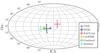 |
Fig. 1. Best-fit dipole directions for individual catalogues NVSS (blue), RACS-low (red), and CatWISE (orange). For the combined fits, the best-fit direction for the full dipole (hypothesis (0) and (i), green) and the residual dipole fixing the kinematic dipole to the CMB dipole (hypothesis (iii), turquoise) are also shown. In all cases, the error bars indicate the 1σ uncertainties. The direction of the CMB dipole is indicated by the black circle and dot. |
4.1. Combined dipole estimates
For a dipole estimate combining NVSS, RACS-low, and CatWISE, the same masks and flux density cuts were used as the estimates on the individual catalogues shown in Table 1. In addition, however, to ensure that these catalogues are statistically independent, we excluded all NVSS sources in the southern hemisphere and all RACS-low sources in the northern hemisphere, such that these catalogues had no overlap. We also cross-matched both NVSS and RACS-low with the CatWISE catalogue and removed sources that match within the angular resolution of the respective catalogues from CatWISE. We thus had three completely independent catalogues with which to perform joint dipole fits. Combining these three catalogues yields 2 035 541 sources, the largest sample used for a dipole estimate thus far. We used the multi-Poisson estimator described in Sect. 2 to obtain best-fit dipole parameters using Eq. (8). We again emphasise that our hypotheses are all based on the assumption that the only kinematic contribution to the combined dipole stems from Eq. (1); that is, no other dipole contributions that scale with β are considered. We discuss the implication of this assumption in Sect. 5.
The designated null hypothesis assumes that the observed dipole is entirely kinematic. This assumption yields a best-fit dipole direction shown by the green cross in Fig. 1. Since CatWISE is contributing more than half of the sources, the direction is closely aligned with the dipole direction of the CatWISE catalogue. The direction is offset from the CMB dipole direction by 23 ± 5 degrees, with a significance level of 4.6σ. As shown in Table 2, the best-fit value for the velocity is β = (2.62 ± 0.26)×10−3 or v = 786 ± 78 km/s, which is a factor of 2.1 larger than the canonical velocity obtained from the CMB dipole. Comparison with the results of the individual catalogues shows that this closely aligns with the possible boost of the CatWISE catalogue, but it differs from the boosts of the NVSS and RACS-low catalogues. Of course, these differences could (to an extent) be due to shot noise. To determine to what extent these latter catalogues disfavour a purely kinematic explanation, we must consider the hypotheses that fit for a non-kinematic component. As our null hypothesis, the marginal likelihood from this fit serves as a baseline against which to compare the other models. Thus, for each subsequent hypothesis we also present the Bayes factor in Table 2; this is defined as the difference between the natural logarithm of the marginal likelihood of that hypothesis and this null hypothesis: lnB = Δln𝒵.
Results and Bayes factors for the different tested hypotheses. Since the fit did not converge for hypothesis (ii), it is not included.
4.2. Separating dipole components
Fitting for hypothesis (i), the best-fit dipole direction is the same as before, shown by the green cross in Fig. 1. Now, in addition to β, the amplitude of a residual, non-kinematic dipole component is also included in the model (given by 𝒟resid). The left panel of Fig. 2 shows the posterior distribution of β and 𝒟resid for this estimate. There is a clear degeneracy between β and 𝒟resid, which is to be expected given that both parameters contribute to the overall dipole. Nevertheless, there is a region of higher likelihood that allows us to constrain the preferred values of β and 𝒟resid, as given in Table 2. The distribution of β is consistent with zero, with β < 2.34 × 10⁻³ at a 95% confidence level (CL). This is, however, also consistent with the canonical velocity from the CMB (β = 1.23 × 10⁻³, indicated by the red line in Fig. 2). At face value, the posterior thus indicates a preference for the kinematic contribution being consistent with or lower than the CMB velocity, rather than with a value of β ∼ 2.6 × 10⁻³, at which the common dipole is fully kinematic and 𝒟resid ∼ 0. Comparing this model to hypothesis (0) quantitatively requires us to account for the additional free parameter. The Bayes factor of lnBi, 0 = −3.0 indicates a preference for the fully kinematic model over this one. Nevertheless, the model itself shows a preference for a non-zero residual dipole, which motivated us to further investigate the possibility of this component being present.
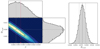 |
Fig. 2. Left: Hypothesis (i). Posterior distribution of β and 𝒟resid from the combined estimate using NVSS, RACS-low, and CatWISE. The 1-,2-, and 3-σ uncertainties are indicated by the black contours. The dotted lines indicate the maximum posterior values for these parameters. The canonical CMB velocity of β = 1.23 × 10⁻³ is indicated by the dotted red line, with the red dot indicating the kinematic dipole expected in the standard cosmology; this is assuming a negligible structure dipole (𝒟resid ≈ 0). Right: Hypothesis (iii). Posterior distribution of 𝒟resid, where the kinematic dipole is fixed to the CMB dipole. We note the respective evidence for and against these posteriors’ hypotheses in Table 2. |
For some additional checks, we performed the same hypothesis (i) fits for a number of different variations on the data sets, the results of which are shown in Appendix A. The top panels of Fig. A.1 show the results of combining each of the radio catalogues separately with CatWISE. Since we do not have to account for overlap between NVSS and RACS-low, we did not restrict each to their respective hemispheres here. These distributions generally favour higher values of β, with peak posteriors closer to the canonical CMB velocity. As such, the fully kinematic dipole is not as disfavoured, while the fully residual dipole is disfavoured. The difference with the result shown in Fig. 2 is likely caused by disagreement between the observed dipole directions of NVSS and RACS-low. Though they are expected to have very similar dipole amplitudes, the difference in the RACS-low and NVSS dipole directions causes the combination of them to have an overall lower dipole amplitude (as was also shown in Wagenveld et al. 2023 and Oayda et al. 2024), which also lowers the inferred value of β, as we see in Fig. 2 (left panel). In the lower panels of Fig. A.1, we again feature all catalogues, but we applied different flux density cuts to the data. The flux limits chosen here were optimised to avoid them being affected by systematics in the catalogue, while still maintaining a sufficient number of sources for the dipole estimate. Nonetheless, it is useful to see the behaviour of these fits for different flux cuts. The lower left panel shows the result if we increase the flux cut of all catalogues, to 20 mJy for NVSS and RACS-low, and 0.09 mJy (W1 < 16.4) for CatWISE (matching Secrest et al. 2021). With this cut, either through a genuine effect or because of shot noise induced by the decreased source density, both NVSS and RACS-low significantly increase in dipole amplitude, resulting in a lower estimate of β. This rather stark difference compared to our other results is surprising and highlights the need for deeper radio catalogues. With the current data, however, it is difficult to say what causes this difference. For completeness, the lower right panel of Fig. A.1 shows the results if sources matched to 2MRS sources at z < 0.1 are removed from all catalogues; though, as mentioned previously, 2MRS is volume-incomplete at redshifts beyond z ≳ 0.02. With the caveats that it is not likely that all z < 0.1 sources are removed and that boundary effects are not accounted for (as discussed in Sect. 3.4), the dipole amplitudes of NVSS and RACS-low are lowered, resulting in higher values of β being preferred in this fit.
If the dipole consists of different components, as Fig. 2 suggests, forcing these components to point in the same direction is potentially too constraining a model. Though generally it has been found that the directions of the overall dipole are consistent with the CMB dipole direction, CatWISE, which has the most discriminating power in a single catalogue, has a dipole direction that is inconsistent with the CMB dipole. Looking at the different dipole directions in Fig. 1, we see that there is a good agreement between the CatWISE and NVSS dipole directions, indicating that if the NVSS measurement were more precise, it might yield this result as well. The RACS-low dipole, however, is offset in a different direction, which makes the case less clear. Because NVSS and RACS-low do not agree in terms of direction, while NVSS and CatWISE agree, this provides little constraints on the directions of the separate dipole components. Freeing up both directions and amplitudes as in hypothesis (ii) thus does not yield a converging estimate. Instead, we reduced hypothesis (ii) to hypothesis (iii), fixing the kinematic dipole both in terms of direction as well as amplitude to the CMB expectation, while leaving the residual dipole completely free.
The resulting direction for the residual dipole is shown in turquoise in Fig. 1, and has an angular separation from the kinematic dipole of 39 ± 8 degrees, with a significance level of 4.6σ. To understand whether this offset could be due to a chance alignment, we can consider two interpretations of alignment and correlation between the dipole component directions. Firstly, we can simply consider the probability of finding two directions on a sphere with a distance of Δθ. For this case, the distance between the different directions can be between 0° (alignment) and 90° (anti-alignment), resulting in the probability of ![Mathematical equation: $ p = \frac{1}{2}[1-\cos(\Delta\theta)] $](/articles/aa/full_html/2025/05/aa53397-24/aa53397-24-eq11.gif) . For this result, the probability of the two directions being within Δθ = 40° of each other is p = 0.12. This, however, does not consider anti-alignment as ‘special’ as alignment, even though anti-alignment can be considered a correlation between the directions to the same degree that an alignment can. For this case, the probability is instead p = 1 − cos(Δθ), doubling the probability for our result to p = 0.24. Thus, with the current results, there is no conclusive evidence as to whether or not the directions of the two dipole components are correlated. However, if 𝒟resid signifies a true density fluctuation on the largest scales, it would not be hard to imagine that this density gradient could (partially) pull all matter along it, in which case an alignment between the kinematic and non-kinematic dipole component is entirely natural. For the amplitude of the residual dipole, the posterior distribution is shown in the right panel of Fig. 2. As also shown in Table 2, this indicates a best-fit 𝒟resid = (0.81 ± 0.14)×10−2, corresponding to a detection significance of 5.4σ. Not surprisingly, this amplitude is consistent with the residual dipole common to the CatWISE AGN and NVSS reported by Secrest et al. (2022). However, the present work also computes the corresponding posterior. Comparing this model to hypothesis (0), we obtain a Bayes factor of lnBiii, 0 = 3.5, indicating this model to be favoured in comparison. This shows that separating the kinematic and non-kinematic component both in terms of amplitude and direction is favourable; however, as mentioned before, converging fits can only be achieved if one component is fixed, which limits the utility of this approach until larger catalogues have been surveyed.
. For this result, the probability of the two directions being within Δθ = 40° of each other is p = 0.12. This, however, does not consider anti-alignment as ‘special’ as alignment, even though anti-alignment can be considered a correlation between the directions to the same degree that an alignment can. For this case, the probability is instead p = 1 − cos(Δθ), doubling the probability for our result to p = 0.24. Thus, with the current results, there is no conclusive evidence as to whether or not the directions of the two dipole components are correlated. However, if 𝒟resid signifies a true density fluctuation on the largest scales, it would not be hard to imagine that this density gradient could (partially) pull all matter along it, in which case an alignment between the kinematic and non-kinematic dipole component is entirely natural. For the amplitude of the residual dipole, the posterior distribution is shown in the right panel of Fig. 2. As also shown in Table 2, this indicates a best-fit 𝒟resid = (0.81 ± 0.14)×10−2, corresponding to a detection significance of 5.4σ. Not surprisingly, this amplitude is consistent with the residual dipole common to the CatWISE AGN and NVSS reported by Secrest et al. (2022). However, the present work also computes the corresponding posterior. Comparing this model to hypothesis (0), we obtain a Bayes factor of lnBiii, 0 = 3.5, indicating this model to be favoured in comparison. This shows that separating the kinematic and non-kinematic component both in terms of amplitude and direction is favourable; however, as mentioned before, converging fits can only be achieved if one component is fixed, which limits the utility of this approach until larger catalogues have been surveyed.
5. Discussion
The cosmic dipole anomaly, namely the unexpectedly large dipole amplitudes found in number counts of galaxies, raises the question of the origin and composition of the observed dipoles. In this work, we were specifically interested in distinguishing kinematic from non-kinematic contributions, or, as written here, 𝒟kin and 𝒟resid, respectively. To this effect, we assumed the Ellis & Baldwin (1984) dipole amplitude (Eq. (1)) to be the only kinematic contribution to the dipole amplitude observed in a given galaxy catalogue; its proportionality to the continuous parameter β allowed us to consider a fit to the observer velocity. Crucial to this work was the factor preceding β being fixed by the respective galaxy catalogue’s properties. Simultaneously, we assumed the residual dipole amplitude to be the same in each of the employed galaxy catalogues. In combination, these assumptions help break the degeneracy otherwise present between β and 𝒟resid (see Eq. (2), or alternatively Eq. (8), which allows individual directions of the constituent dipoles).
The idea of a common residual dipole in different catalogues was initially explored in Secrest et al. (2022), which simply compared the dipoles found in the NVSS and CatWISE samples before and after subtraction of the expected kinematic dipole. Assuming the canonical observer velocity taken from the CMB dipole yielded nearly matching values of 𝒟resid for both catalogues, sparking our hypothesis (iii). Our work essentially formalises this comparison, accounting for uncertainties in amplitudes and directions consistently. By including the RACS-low catalogue, we further extended this ansatz to more data, using the additional sky coverage and accompanying scrutinising power. And yet, with this compilation of data neither a purely kinematic nor a purely residual dipole can be conclusively excluded if the kinematic component is indeed entirely determined by Eq. (1). Nevertheless, we find that the most preferred model is one where the kinematic component of the number-count dipole is close to or lower than the purely kinematic interpretation of the CMB dipole (i.e. β ∼ 1.23 × 10⁻³). The remainder of the number-count dipole is correspondingly made up by the residual, non-kinematic dipole.
The general idea to separate kinematic- from non-kinematic matter dipole contributions is not unique to this work. A number of observables have been considered for this purpose in recent years. For example, weighted number counts can be constructed in a way to separate an intrinsic ‘clustering’ component from that expected due to the observer boost alone (Nadolny et al. 2021); these are yet to be applied to suitable data with redshift estimates. However, even utilising redshift measurements alone, without the collection of number counts, can provide a handle on the observer’s velocity as per the induced Doppler shifts on the redshifts. This was recently applied to data from the SDSS by Ferreira & Marra (2024) and, in an attempt to reproduce their results, by Tiwari et al. (2024). While some sub-samples deliver measurements of β in agreement with the value derived from the CMB dipole, other sub-samples do not provide similar constraints, and their methods do not yet appear to match the subtleties of the data. Lastly, the angular aberration induced by the observer boost that leads to the factor of two in Eq. (1) might also be considered in an isolated manner when studying source counts. This was worked out theoretically by Lacasa et al. (2024) with good prospects for upcoming surveys to constrain β and, therewith, our velocity with respect to the matter rest frame.
5.1. Assumptions on the present work
It is valuable to highlight what might violate the assumptions made for this analysis. Firstly, contributions to the expected dipole amplitudes that scale with β in addition to those of Eq. (1) would undermine the premise of our analysis. To date, no such contributions are known for galaxy catalogues as those investigated here. While it has recently been suggested that redshift evolution of the catalogues’ source populations might lead to effects beyond Eq. (1) and also proportional to β (e.g. Dalang & Bonvin 2022; Guandalin et al. 2023), these seemingly generalising effects have been shown (von Hausegger 2024) to already be fully included in the Ellis & Baldwin (1984) amplitude (Eq. (1)) used all along. Specifically, as the catalogues treated here are redshift-integrated, so are the aforementioned redshift-evolution effects, reducing any redshift evolving parameter (such as x or α) to a well-defined average, so long as this is measured at the corresponding flux limit of each catalogue. Central to this conclusion is the understanding that any luminosity function describing the sources in redshift must also describe the unique redshift-integrated source counts that are actually observed, which had not been considered in the proposition by Dalang & Bonvin (2022) and Guandalin et al. (2023). While additional, kinematic terms are expected in, for example, redshift tomographic measurements (von Hausegger & Dalang 2024), fully redshift-integrated catalogues such as those described here (barring the z < 0.02 cut, which we estimate to have a negligible effect) are again not known to require any corrections to Eq. (1), justifying our first defining assumption.
Our second assumption states that the residual dipole is present in all surveys with the same amplitude and direction. Of course, there is no way to know whether this assumption is accurate in light of the fact that we do not know what the residual dipole truly is or even if it exists. As mentioned above, this was motivated by the observation in Secrest et al. (2022). In this sense, it is not surprising that we recovered posteriors for β that appear to have peaked close to the canonical velocity. Assuming the residual dipole to be different per survey, for instance by considering it to originate from random shot noise that is not insubstantial for the given catalogue sizes, leads to our considered hypothesis (0). This hypothesis yields a recovered value for β that lies at around twice the canonical value. While the posteriors and Bayes factors comparing the models with and without a residual dipole favour the former option, the evidence is not strong enough to be considered conclusive. Also, a residual dipole that somehow varies per catalogue, for instance as a function of frequency (as suggested by Siewert et al. 2020), invalidates this assumption, although this would still require a non-kinematic component to be present. Clearly, the natural degeneracy of 𝒟kin and 𝒟resid is only broken if an additional assumption on the stability of 𝒟resid is made. However, should future theoretical investigations predict a common, non-kinematic contribution to the matter dipoles across samples, then our work offers a prediction of just this.
5.2. The multi-wavelength dipole
In this work, we used catalogues gathered at different wavelengths to constrain the dipole and its components. With this choice of catalogues, we implicitly combined different objects: Quasars at mid-IR frequencies and predominantly AGN at the radio frequencies. Though they are observationally distinct, these source samples are all part of the active galaxies class and therefore have similar redshift distributions, with a median of z ∼ 1 (e.g. Secrest et al. 2021; Tiwari & Nusser 2016). Going forward, however, when fainter sources (especially in the radio) are included in these studies, SFGs will begin to dominate the radio samples. These will present a wholly different source population, for which a residual dipole might deviate to a significant degree (for a recent example, see Wagenveld et al. 2024). One might thus attempt to interpret 𝒟resid as a clustering dipole, making studies of galaxy bias paramount (see Peebles 2022) in light of the diversity of galaxy types inherent to the different samples.
Nonetheless, this difference in frequency consequently means that instrumental systematics do not offer a plausible explanation for these dipoles, not only due to the vastly different experimental details of NVSS, RACS-low, and CatWISE, respectively, but also the range in frequencies by which the radio and mid-IR measurements differ. The residual dipole entertained here is not to be interpreted as systematic. Rather, it is a reframing of the upheld cosmic dipole anomaly in a quest to understand its cosmological origin. Independent of the decomposition of the observed dipoles into kinematic and residual contributions, the conclusion that 𝒟obs is too large to be reconcilable with the cosmological principle remains.
5.3. Theoretical context
If the kinematic dipole is that expected from the kinematic interpretation of the CMB dipole, as is hinted at by our analysis, the corresponding residual dipole is too large to be explained within the linear perturbations expected in the standard cosmological model. In other words, the clustering contributions to the number-count dipole in the high-redshift samples investigated here, as predicted within Λ-CDM, are smaller than the inferred residual dipole seen by a factor of a few tens (depending on the galaxy bias b(z); Gibelyou & Huterer 2012; Secrest et al. 2021).
Thus, the question as to which phenomenon would produce a non-kinematic 𝒟resid still stands. To understand the difference between CMB dipole and the corresponding expected dipole in galaxy number counts, one may consider the presence of large horizon-sized density perturbations. It is known that an adiabatic mode of such a scale does not alter the CMB dipole, compared with what is expected due to our currently understood observer velocity (e.g. Grishchuk & Zeldovich 1978; Erickcek et al. 2008). Instead, this sparked studies into iso-curvature modes (e.g. Gunn 1988; Turner 1991, 1992; Langlois & Piran 1996; Erickcek et al. 2009), which do cause a sought-after difference by adding a non-vanishing, intrinsic dipole component to that of the CMB. Regarding the number-count dipole, however, Domènech et al. (2022) find that neither adiabatic, nor iso-curvature perturbations can be associated with a number-count dipole as large as those observed, if β remains at its canonical value. One must therefore, if considering a substantial non-kinematic 𝒟resid, speculate about other phenomenology on large scales, such as non-Gaussianity or effects of non-linear growth.
5.4. Outlook
While awaiting larger cosmological surveys such as Rubin-LSST, Euclid, or SKA, we are currently in a situation where analyses of data sets in synergy offer the best attempt to understand the origin of the cosmic dipole anomaly. As such, it is worth noting here that the excess dipole is not the only potentially problematic anisotropy that has been observed so far. Particularly noteworthy in this context are the anisotropies seen in the scaling relations of X-ray clusters (Migkas & Reiprich 2018; Migkas et al. 2021), which are either linked to anisotropic Hubble expansion or bulk flows beyond the scale of what is expected in a homogeneous and isotropic universe. Excess bulk flows have also been seen in other data sets (Watkins et al. 2023). It is very possible that these anisotropies are connected to the ones mentioned here as well as other observed cosmological inconsistencies (see Aluri et al. 2023 for an overview). However, considering the results obtained here, especially the constraints on β obtained with hypothesis (i), a measured β below the canonical velocity is fully consistent with our constraints, and could be obtained if the observed source population is also moving with respect to the CMB rest frame. This would be in line with an excess bulk flow, although it would have to be sustained to much larger scales than the currently available velocity data.
In this work, we considered combinations of three data sets that to-date have delivered the most robust measurements on the number-count dipoles; in total, this adds up to about 2.3 million sources. Yet, even after having combined these current data sets, the width of the posteriors remained too broad to conclusively distinguish a kinematic from a non-kinematic origin of the observed matter dipoles. Nevertheless, we demonstrated the feasibility of this distinction exclusively with galaxy number counts by leveraging the sample-dependent kinematic matter dipole expectation, Eq. (1), and by considering different assumptions on an additional, non-kinematic, residual dipole component.
6. Conclusion
In this paper, we leveraged the differences between the expected kinematic dipole amplitudes of different catalogues to try to isolate the kinematic dipole from a possible residual dipole effect. To this effect, we assumed that the only kinematic contribution to the number-count dipole is given by the Ellis & Baldwin (1984) amplitude (Eq. (1)), which allowed us to separate kinematic from non-kinematic dipole contributions. Differences between the expectations for different catalogues are caused by different values of x and α in each catalogue. To this end, we used the radio catalogues of NVSS and RACS-low and the infrared CatWISE catalogue. These catalogues have previously yielded robust measurements of the cosmic number-count dipole individually, and therefore formed our primary selection of data sets, whereas other data sets individually delivered less significant dipole measurements. Furthermore, with some minor cuts, the catalogues cover the whole sky twice over while being entirely independent. With this, the different catalogues could be combined for a joint dipole estimation as previously defined in Wagenveld et al. (2023).
Using the different expected kinematic dipole amplitudes for the catalogues, we fitted for the kinematic and residual dipoles separately. Although freeing up both amplitudes and directions of these dipoles did not yield a converging estimate, letting the different dipole components have a common direction but different amplitudes did. The resulting posterior indicated a preference for a lower kinematic dipole component with β < 2.35 × 10⁻³ (95% CL), which is consistent with the canonical velocity taken from the CMB dipole. Consequently, as per Eq. (2), the remaining excess dipole amplitude was found to be in the form of a residual dipole, the origin of which is not known. Freeing up the parameters of the residual dipole while fixing those of the kinematic dipole to the CMB values, we found a residual dipole offset from the CMB direction by 39 ± 8 degrees, with an amplitude of 𝒟resid = (0.81 ± 0.14)×10−2, deviating from a non-existent residual dipole by 5.5σ. Evidently, this significance level simply reflects a rephrasing of the notorious dipole anomaly. Furthermore, this interpretation appeared to be more favourable than the other hypotheses according to the computed Bayesian evidence.
It is enticing to have found a preference for the interpretation that the observed number-count dipole in different radio, infrared, and optical surveys consists of a kinematic component that matches the velocity derived from the CMB dipole along with a residual, non-kinematic dipole. The catalogues employed here do not have the sensitivity required to fully break the degeneracy between the different dipole components, calling for a repeat measurement with a future set of deeper – but still independent – catalogues. Deeper radio catalogues, both in the northern and southern hemispheres, would be particularly useful, as here CatWISE dominates the estimates, especially in terms of direction.
Here, we use the spectral index convention S ∝ ν−α.
We can estimate that, for a catalogue such as NVSS, the removal of sources with redshifts of z < 0.02 leads to a reduction of the expected dipole amplitude of 𝒪(1%), whereas when z < 0.1 the reduction is 𝒪(10%).
Acknowledgments
We thank the anonymous referee for their insightful comments and feedback. Some of the results in this paper have been derived using the HEALPY (Zonca et al. 2019) and HEALP IX (Górski et al. 2005) packages. This research has made use of TOPCAT (Taylor 2005), BILBY (Ashton et al. 2019), EMCEE (Foreman-Mackey et al. 2013), and HARMONIC (McEwen et al. 2021).
References
- Aluri, P., Cea, P., Chingangbam, P., et al. 2023, CQG, 40, 094001 [NASA ADS] [CrossRef] [Google Scholar]
- Ashton, G., Hübner, M., Lasky, P. D., et al. 2019, ApJS, 241, 27 [NASA ADS] [CrossRef] [Google Scholar]
- Blake, C., & Wall, J. 2002, Nature, 416, 150 [NASA ADS] [CrossRef] [Google Scholar]
- Colin, J., Mohayaee, R., Rameez, M., & Sarkar, S. 2017, MNRAS, 471, 1045 [Google Scholar]
- Condon, J. J. 1984, ApJ, 287, 461 [Google Scholar]
- Condon, J. J., Cotton, W. D., Greisen, E. W., et al. 1998, AJ, 115, 1693 [Google Scholar]
- Crawford, F. 2009, ApJ, 692, 887 [NASA ADS] [CrossRef] [Google Scholar]
- Dalang, C., & Bonvin, C. 2022, MNRAS, 512, 3895 [NASA ADS] [CrossRef] [Google Scholar]
- Dam, L., Lewis, G. F., & Brewer, B. J. 2023, MNRAS, 525, 231 [NASA ADS] [CrossRef] [Google Scholar]
- Darling, J. 2022, ApJ, 931, L14 [NASA ADS] [CrossRef] [Google Scholar]
- Domènech, G., Mohayaee, R., Patil, S. P., & Sarkar, S. 2022, JCAP, 2022, 019 [CrossRef] [Google Scholar]
- Duchesne, S. W., Thomson, A. J. M., Pritchard, J., et al. 2023, PASA, 40, e034 [NASA ADS] [CrossRef] [Google Scholar]
- Ellis, G. F. R., & Baldwin, J. E. 1984, MNRAS, 206, 377 [NASA ADS] [CrossRef] [Google Scholar]
- Erickcek, A. L., Carroll, S. M., & Kamionkowski, M. 2008, Phys. Rev. D, 78, 083012 [Google Scholar]
- Erickcek, A. L., Hirata, C. M., & Kamionkowski, M. 2009, Phys. Rev. D, 80, 083507 [Google Scholar]
- Ferreira, P. d. S., & Marra, V. 2024, JCAP, 077, 2024 [Google Scholar]
- Ferreira, P. d. S., & Quartin, M. 2021, Phys. Rev. Lett., 127, 101301 [NASA ADS] [CrossRef] [Google Scholar]
- Foreman-Mackey, D., Hogg, D. W., Lang, D., & Goodman, J. 2013, PASP, 125, 306 [Google Scholar]
- Gibelyou, C., & Huterer, D. 2012, MNRAS, 427, 1994 [NASA ADS] [CrossRef] [Google Scholar]
- Górski, K. M., Hivon, E., Banday, A. J., et al. 2005, ApJ, 622, 759 [Google Scholar]
- Grishchuk, L. P., Zeldovich, I. A. B., 1978, Soviet Ast., 22, 125 [Google Scholar]
- Guandalin, C., Piat, J., Clarkson, C., & Maartens, R. 2023, ApJ, 953, 144 [Google Scholar]
- Gunn, J. E. 1988, ASP Conf. Ser., 4, 344 [NASA ADS] [Google Scholar]
- Hale, C. L., McConnell, D., Thomson, A. J. M., et al. 2021, PASA, 38, e058 [NASA ADS] [CrossRef] [Google Scholar]
- Horstmann, N., Pietschke, Y., & Schwarz, D. J. 2022, A&A, 668, A34 [NASA ADS] [CrossRef] [EDP Sciences] [Google Scholar]
- Huchra, J. P., Macri, L. M., Masters, K. L., et al. 2012, ApJS, 199, 26 [Google Scholar]
- Lacasa, F., Bonvin, C., Dalang, C., & Durrer, R. 2024, JCAP, 2024, 045 [CrossRef] [Google Scholar]
- Lacy, M., Baum, S. A., Chandler, C. J., et al. 2020, PASP, 132, 035001 [Google Scholar]
- Langlois, D., & Piran, T. 1996, Phys. Rev. D, 53, 2908 [Google Scholar]
- Marocco, F., Eisenhardt, P. R. M., Fowler, J. W., et al. 2021, ApJS, 253, 8 [Google Scholar]
- McConnell, D., Hale, C. L., Lenc, E., et al. 2020, PASA, 37, e048 [Google Scholar]
- McEwen, J. D., Wallis, C. G. R., Price, M. A., & Spurio Mancini, A. 2021, arXiv e-prints [arXiv:2111.12720] [Google Scholar]
- Migkas, K., & Reiprich, T. H. 2018, A&A, 611, A50 [NASA ADS] [CrossRef] [EDP Sciences] [Google Scholar]
- Migkas, K., Pacaud, F., Schellenberger, G., et al. 2021, A&A, 649, A151 [NASA ADS] [CrossRef] [EDP Sciences] [Google Scholar]
- Mittal, V., Oayda, O. T., & Lewis, G. F. 2024a, MNRAS, 530, 4763 [NASA ADS] [CrossRef] [Google Scholar]
- Mittal, V., Oayda, O. T., & Lewis, G. F. 2024b, MNRAS, 527, 8497 [Google Scholar]
- Nadolny, T., Durrer, R., Kunz, M., & Padmanabhan, H. 2021, JCAP, 2021, 009 [CrossRef] [Google Scholar]
- Oayda, O. T., Mittal, V., Lewis, G. F., & Murphy, T. 2024, MNRAS, 531, 4545 [NASA ADS] [CrossRef] [Google Scholar]
- Oayda, O. T., Mittal, V., & Lewis, G. F. 2025, MNRAS, 537, 1 [NASA ADS] [Google Scholar]
- Peebles, P. J. E. 2022, Ann. Phys., 447, 169159 [NASA ADS] [CrossRef] [Google Scholar]
- Planck Collaboration XXVII. 2014, A&A, 571, A27 [NASA ADS] [CrossRef] [EDP Sciences] [Google Scholar]
- Planck Collaboration I. 2020, A&A, 641, A1 [NASA ADS] [CrossRef] [EDP Sciences] [Google Scholar]
- Rameez, M., Mohayaee, R., Sarkar, S., & Colin, J. 2018, MNRAS, 477, 1772 [Google Scholar]
- Rubart, M., & Schwarz, D. J. 2013, A&A, 555, A117 [NASA ADS] [CrossRef] [EDP Sciences] [Google Scholar]
- Saha, S., Shaikh, S., Mukherjee, S., Souradeep, T., & Wandelt, B. D. 2021, JCAP, 2021, 072 [CrossRef] [Google Scholar]
- Secrest, N. J., von Hausegger, S., Rameez, M., et al. 2021, ApJ, 908, L51 [Google Scholar]
- Secrest, N. J., von Hausegger, S., Rameez, M., Mohayaee, R., & Sarkar, S. 2022, ApJ, 937, L31 [NASA ADS] [CrossRef] [Google Scholar]
- Siewert, T. M., Hale, C., Bhardwaj, N., et al. 2020, A&A, 643, A100 [EDP Sciences] [Google Scholar]
- Siewert, T. M., Schmidt-Rubart, M., & Schwarz, D. J. 2021, A&A, 653, A9 [NASA ADS] [CrossRef] [EDP Sciences] [Google Scholar]
- Singal, A. K. 2011, ApJ, 742, L23 [NASA ADS] [CrossRef] [Google Scholar]
- Taylor, M. B. 2005, ASP Conf. Ser., 347, 29 [Google Scholar]
- Tiwari, P., & Nusser, A. 2016, JCAP, 2016, 062 [Google Scholar]
- Tiwari, P., Kothari, R., Naskar, A., Nadkarni-Ghosh, S., & Jain, P. 2015, Astropart. Phys., 61, 1 [Google Scholar]
- Tiwari, P., Schwarz, D. J., Zhao, G.-B., et al. 2024, ApJ, 975, 279 [Google Scholar]
- Turner, M. S. 1991, Phys. Rev. D, 44, 3737 [NASA ADS] [CrossRef] [Google Scholar]
- Turner, M. S. 1992, Gen. Rel. Grav., 24, 1 [Google Scholar]
- von Hausegger, S. 2024, MNRAS, 535, L49 [Google Scholar]
- von Hausegger, S., & Dalang, C. 2024, arXiv e-prints [arXiv:2412.13162] [Google Scholar]
- Wagenveld, J. 2025, https://doi.org/10.5281/zenodo.14965453 [Google Scholar]
- Wagenveld, J. D., Klöckner, H.-R., & Schwarz, D. J. 2023, A&A, 675, A72 [NASA ADS] [CrossRef] [EDP Sciences] [Google Scholar]
- Wagenveld, J. D., Klöckner, H. R., Gupta, N., et al. 2024, A&A, 690, A163 [NASA ADS] [CrossRef] [EDP Sciences] [Google Scholar]
- Watkins, R., Allen, T., Bradford, C. J., et al. 2023, MNRAS, 524, 1885 [NASA ADS] [CrossRef] [Google Scholar]
- Wright, E. L., Eisenhardt, P. R., Mainzer, A. K., et al. 2010, AJ, 140, 1868 [Google Scholar]
- Zonca, A., Singer, L. P., Lenz, D., et al. 2019, J. Open Source Software, 4, 1298 [NASA ADS] [CrossRef] [Google Scholar]
Appendix A: Additional combined dipole estimates
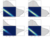 |
Fig. A.1. Posterior distributions of β and 𝒟resid. Top left: Using only NVSS and CatWISE. Top right: Using only RACS-low and CatWISE. Bottom left: With higher flux density cuts applied, 20 mJy for NVSS and RACS-low, and 0.09 mJy (W1 < 16.4) for CatWISE. Bottom right: With sources at z < 0.1 in 2MRS removed from all catalogues. The 1,2, and 3σ uncertainties are indicated by the black contours. The dotted line indicates the maximum posterior values for these parameters. The canonical CMB velocity of β = 1.23 × 10⁻³ is indicated by the dotted red line, the red dot indicating the kinematic dipole expected in the standard cosmology, assuming a negligible structure dipole (𝒟resid ≈ 0) |
Best-fit dipole estimates for different data combinations and cuts. When catalogues are combined, only hypothesis (i) is tested, with results shown in Fig. A.1.
All Tables
Results and Bayes factors for the different tested hypotheses. Since the fit did not converge for hypothesis (ii), it is not included.
Best-fit dipole estimates for different data combinations and cuts. When catalogues are combined, only hypothesis (i) is tested, with results shown in Fig. A.1.
All Figures
|
Fig. 1. Best-fit dipole directions for individual catalogues NVSS (blue), RACS-low (red), and CatWISE (orange). For the combined fits, the best-fit direction for the full dipole (hypothesis (0) and (i), green) and the residual dipole fixing the kinematic dipole to the CMB dipole (hypothesis (iii), turquoise) are also shown. In all cases, the error bars indicate the 1σ uncertainties. The direction of the CMB dipole is indicated by the black circle and dot. |
| In the text | |
|
Fig. 2. Left: Hypothesis (i). Posterior distribution of β and 𝒟resid from the combined estimate using NVSS, RACS-low, and CatWISE. The 1-,2-, and 3-σ uncertainties are indicated by the black contours. The dotted lines indicate the maximum posterior values for these parameters. The canonical CMB velocity of β = 1.23 × 10⁻³ is indicated by the dotted red line, with the red dot indicating the kinematic dipole expected in the standard cosmology; this is assuming a negligible structure dipole (𝒟resid ≈ 0). Right: Hypothesis (iii). Posterior distribution of 𝒟resid, where the kinematic dipole is fixed to the CMB dipole. We note the respective evidence for and against these posteriors’ hypotheses in Table 2. |
| In the text | |
|
Fig. A.1. Posterior distributions of β and 𝒟resid. Top left: Using only NVSS and CatWISE. Top right: Using only RACS-low and CatWISE. Bottom left: With higher flux density cuts applied, 20 mJy for NVSS and RACS-low, and 0.09 mJy (W1 < 16.4) for CatWISE. Bottom right: With sources at z < 0.1 in 2MRS removed from all catalogues. The 1,2, and 3σ uncertainties are indicated by the black contours. The dotted line indicates the maximum posterior values for these parameters. The canonical CMB velocity of β = 1.23 × 10⁻³ is indicated by the dotted red line, the red dot indicating the kinematic dipole expected in the standard cosmology, assuming a negligible structure dipole (𝒟resid ≈ 0) |
| In the text | |
Current usage metrics show cumulative count of Article Views (full-text article views including HTML views, PDF and ePub downloads, according to the available data) and Abstracts Views on Vision4Press platform.
Data correspond to usage on the plateform after 2015. The current usage metrics is available 48-96 hours after online publication and is updated daily on week days.
Initial download of the metrics may take a while.