| Issue |
A&A
Volume 675, July 2023
|
|
|---|---|---|
| Article Number | A140 | |
| Number of page(s) | 9 | |
| Section | Stellar structure and evolution | |
| DOI | https://doi.org/10.1051/0004-6361/202345935 | |
| Published online | 11 July 2023 | |
Recurrent mini-outbursts and a magnetic white dwarf in the symbiotic system FN Sgr
1
Advanced Technologies Research Institute, Faculty of Materials Science and Technology in Trnava, Slovak University of Technology in Bratislava, Bottova 25, 917 24 Trnava, Slovakia
e-mail: This email address is being protected from spambots. You need JavaScript enabled to view it.
2
Department of Astronomy, University of Wisconsin, 475 N. Charter Str., Madison, WI 53706, USA
3
INAF – Astronomical Observatory Padova, Vicolo dell’Osservatorio 5, 35122 Padova, Italy
4
Nicolaus Copernicus Astronomical Center, Polish Academy of Sciences, Bartycka 18, 00-716 Warsaw, Poland
5
Kleinkaroo Observatory, Calitzdorp, Western Cape, South Africa
6
Department of Physics and Kavli Institute for Astrophysics and Space Research, Massachusetts Institute of Technology, 77 Massachusetts Avenue, Cambridge, MA 02139, USA
Received:
18
January
2023
Accepted:
31
May
2023
Abstract
Aims. We investigated the optical variability of the symbiotic binary FN Sgr with photometric monitoring over a period of ≃55 years and with a high-cadence Kepler light curve lasting 81 days.
Methods. The data obtained in the V and I bands were reduced with standard photometric methods. The Kepler data were divided into subsamples and were analysed with the Lomb-Scargle algorithm.
Results. The V and I band light curves show a phenomenon never before observed with such recurrence in any symbiotic system, namely short outbursts starting between orbital phases 0.3 and 0.5 and lasting about 1 month, with a fast rise, a slower decline, and amplitudes of 0.5–1 mag. In the Kepler light curve, we discovered three frequencies with sidebands. We attribute a stable frequency of 127.5 d−1 (corresponding to a period of 11.3 min) to the white dwarf rotation. We suggest that this detection probably implies that the white dwarf accretes through a magnetic stream, as in intermediate polars. The small outbursts may be ascribed to the stream–disc interaction. Another possibility is that they are due to localised thermonuclear burning, perhaps confined by the magnetic field, such as those recently inferred in intermediate polars, albeit on different timescales. We also measured a second frequency around 116.9 d−1 (corresponding to about 137 min), which is much less stable and has a drift. This latter may be due to rocky detritus around the white dwarf, but is more likely caused by an inhomogeneity in the accretion disc. Finally, there is a third frequency close to the first one that appears to correspond to the beating between the rotation and the second frequency.
Key words: accretion, accretion disks / binaries: symbiotic / stars: individual: FN Sgr
© The Authors 2023
 Open Access article, published by EDP Sciences, under the terms of the Creative Commons Attribution License (https://creativecommons.org/licenses/by/4.0), which permits unrestricted use, distribution, and reproduction in any medium, provided the original work is properly cited.
This article is published in open access under the Subscribe to Open model. This email address is being protected from spambots. You need JavaScript enabled to view it. to support open access publication.
1. Introduction
Symbiotic stars are binary systems and are usually comprised of a white dwarf (WD), main sequence, or neutron star, and an evolved companion, namely a red giant (S-type systems), an asymptotic giant branch star, or a Mira variable (D-type systems). The matter from the companion is accreted by the compact object via a stellar wind or Roche lobe overflow, in many cases creating an accretion disc. The orbital periods are ∼200–1000 days for S-type systems and ≳50 years for D-type systems (Mikołajewska 2012).
FN Sgr has mainly been studied spectroscopically (Barba et al. 1992; Munari & Buson 1994; Brandi et al. 2005). Munari & Buson (1994) found some evidence that this WD may be steadily burning accreted hydrogen near its surface. Brandi et al. (2005) presented over 30 years of long-term photometric data and derived an orbital period of 568.3 days, which is supported by a spectroscopic analysis. As we discuss below, we were able to slightly revise this period. Brandi et al. (2005) determined the interstellar extinction (E(B − V) = 0.2 ± 0.1), a distance of about 7 kpc – assuming that the giant fills or almost fills the Roche lobe–, and an orbital inclination of 80°. These latter authors found that FN Sgr is an S-type symbiotic star composed of an M 5-type giant of 1.5 M⊙ with a radius of 140 R⊙ and a hot WD of 0.7 M⊙ with binary separation of 1.6 AU. Brandi et al. (2005) also concluded that the mass-transfer process is most likely caused by the Roche lobe overflow of the red giant. An accretion disc is likely to be present and is most likely the source of the spectral features. Brandi et al. (2005) discuss the double-temperature structure of the hot component – as already observed in other symbiotic stars – as possibly due to a geometrically and optically thick accretion disc. Brandi et al. (2005) discovered a 1996 optical outburst with a 2.5 mag amplitude that lasted until early 2001. Although outbursts are not unusual in symbiotic stars, the temperature and luminosity evolution of the hot component during this outburst were found to be inconsistent with an accretion-disc instability and were difficult to explain (Brandi et al. 2005).
As the only high-time-resolution light curve available – which lasts only 2.8 h (Sokoloski & Bildsten 1999) – is not suitable for a detailed timing analysis, we obtained a high-cadence Kepler light curve, which was measured over 81 days, between 2015 October and December, in Kepler K2 field 7.
2. Observations
The optical data in Fig. 1 include data from Brandi et al. (2005) and the All-Sky-Automated Survey (ASAS, see Gromadzki et al. 2013), and we obtained new photometry with the 35 cm Meade RCX400 telescope at the Kleinkaroo Observatory using a SBIG ST8-XME CCD camera and V and Ic filters. The new V light curve we obtained starts at MJD1 53308, but the Ic data cover a shorter period starting at MJD 56233. Each observation was the result of several individual exposures that were calibrated (dark-subtraction and flat-fielding) and stacked. The magnitudes were derived from differential photometry with nearby reference stars using the single-image mode of the AIP4 image-processing software. The photometric accuracy of the derived magnitudes is better than 0.1 mag.
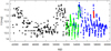 |
Fig. 1. Optical light curve of FN Sgr. Data from (Brandi et al. 2005) are shown in black, the ASAS data in green, and our new data in blue. The Kepler light curve is also shown in red, offset vertically by 12 mag for comparison with the V-band data. |
The Kepler light curve was measured on 5 October 2015 (EPIC 218331937) and is shown in red in Fig. 2. Before flux normalization, systematic corrections were applied following Vanderburg & Johnson (2014) and Vanderburg et al. (2016)2, namely background and barycentric correction. We transformed the flux to magnitudes using the equation: m = −2.5log(f/f0), where f corresponds to the flux value and f0 was set to 1 (not the standardised Kepler response function). A vertical offset of 12 was used to compare the Kepler and V magnitudes.
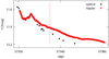 |
Fig. 2. Kepler light curve (red points) with optical data from Fig. 1. The red dashed line shows the superior conjunction of the red giant. |
3. Long-term light curve
The optical V light curve shown in Fig. 1 – with all the data we could gather at this stage – covers almost 55 years. The minima represent the inferior spectroscopic conjunction of the red giant (Brandi et al. 2005). We used all available photometric measurements, including the additional data shown in Fig. 2 (Gromadzki et al. 2013) and revised the ephemeris of the minimum as follows:

where E is the number of orbital cycles, implying that the orbital period is one day shorter than calculated earlier, that is, 567.3 days. The blue dashed lines in Fig. 3 show the minima with a reference minimum determined using a sixth-order polynomial (indicated as a blue thick line). The corresponding superior conjunctions are indicated by red dashed lines.
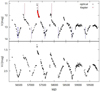 |
Fig. 3. Selected time interval of V light curve from Fig. 1, and corresponding V − I index. The blue and red dashed lines correspond to the inferior and superior conjunction of the red giant, respectively. The blue thick dashed line is the reference optical minimum determined by polynomial fitting. |
In Fig. 1 and in the selected interval in Fig. 3, it is clear that small-amplitude flares, that is those of amplitudes of 0.5–1 mag – which we refer to here as mini-outbursts to differentiate them from major ones such as the 1997–1998 event – occurred between 2001 and 2019 and seem to have ceased in 2020–2021. The ASAS light curve (Gromadzki et al. 2013) indicates that the mini-outbursts occurred since 2001.
Figure 3 shows that these outbursts have a sharp rise (∼10 days) and slower decline, and seem to be orbitally phase-locked. The rise usually starts near phase 0.3 and never after phase 0.5. The bottom panel of Fig. 3 shows that the peak wavelength during the mini-outbursts was shifted towards higher energies, as V − I clearly decreases in magnitude in the flares.
Since 2019, the mini-outburst activity has ceased, and the light curves in addition to the deep eclipses show secondary minima, which are most likely due to ellipsoidal variability. This is particularly evident in the I light curve, in which the red giant significantly contributes to the continuum and confirms the conclusion by Brandi et al. (2005) that the red giant fills (or almost fills) its Roche lobe, as these latter authors inferred from the analysis of the shape and duration of the well-defined eclipses during the large outburst in 1996–2001. If the Roche lobe is filled, a persistent accretion disc should be present in this system.
4. Timing analysis of the Kepler light curve
Our Kepler light curve was observed over 81 days with a cadence of almost 1 min. Such a high-quality and long light curve is ideal for period analysis. The 81 day Kepler run shown in detail in Fig. 2 occurred during the decay from a mini-outburst, as shown in Figs. 1 and 3. Therefore, in addition to orbital variability, a decay after the flare is observed, with a few outlier points due to cosmic rays. To eliminate these effects, first the Hampel filter3 was used to detect and remove outliers. By specifying the size of the window as 61 (30 points on each side + 1 central point), the central point inside this window was replaced by the median value of the window if it differed by more than 5σ from this latter. Next, in order to detrend the light curve, we used a moving window median4 with a window size of 201 (100 points on each side + 1 central point) because a polynomial detrend performed poorly for such a long observation. The window slides over the entire light curve point by point, where the central point is replaced with a median value calculated over the window. Subsequently, we applied the Lomb-Scargle (LS) method by Scargle (1982) to the processed light curve5.
The resulting periodogram shows several peaks above the 90% confidence level (Fig. 4). We show in Fig. 5 that by zooming onto the most significant frequencies, namely 10.5 d−1 (f0), 116.9 d−1 (f1), and 127.5 d−1 (f2), we observe a multi-peak pattern for f0 and f1. Such a drift in frequency is typical for a quasi-periodic signal, and therefore these frequencies may not be stable. On the contrary, f2 exhibits only a single dominant peak, suggesting a stable frequency.
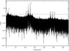 |
Fig. 4. LS periodogram with power in logarithmic scale. The red dashed line indicates the 90% confidence level. |
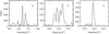 |
Fig. 5. Peak pattern of the f0, f1, and f2 frequencies given by the LS periodogram. |
To determine the origin and the exact behaviour of these frequencies, we split the corrected light curve into 20 portions; 2 equally large parts between days 0 and 10, and 18 equally large parts observed between days 10 and 80. This selection was made in order to distinguish the U-shaped trend at the beginning of the light curve. Subsequently, LS periodograms were created for each portion. First, we inspected the f0, f1, and f2 frequencies. By fitting a Gaussian (or multiple Gaussians where needed), we estimated the frequencies and their uncertainties, which are given in Table 1. The missing values in the f0 column indicate that the peak confidence fell below 90%. On the contrary, two values are instead listed if two close frequencies above 90% confidence were present (double-peak). We then calculated the mean (with the whole light curve) of the two main frequencies f1 and f2. By subtracting f2 from f1 we found the difference Δ(f)≈10.66 d−1, which is very close to the f0 peak. The LS periodogram for each portion of the light curve, with mean frequencies indicated by vertical lines, is shown for f1 and f2 in Fig. 6, and the Δ value for f0 is also indicated.
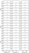 |
Fig. 6. LS periodogram per portion, obtained by dividing the Kepler light curve into 20 equally spaced sub-samples. The first column represents f0, the second f1, and the third f2. The vertical lines indicate the mean value of f1 and f2, or Δ when f0 was computed as the difference between the two frequencies. |
Gaussian frequencies fit.
By examining Table 1 and Fig. 6, we observe the trends of the frequencies. The lower frequency f0 exhibits a visible drift around the Δ value. Moreover, the frequency disappeared at certain times, as its power fell below the 90% confidence level. A similar behaviour is observed for f1, where the peaks drift around the mean value. On the other side, we can see an obvious decline in power in the second half of the light curve, although it is still above the selected confidence level. Only the f2 frequency appears to be stable; its drift around the mean is minimal, and so is the decrease in power. In Sect. 5, we discuss the interpretation of the results in more detail.
To confirm that the detrending using a median filter did not suppress any hidden variability within the light curve, we performed a polynomial detrend for each portion of the light curve. A polynomial fitted the short subsamples much better than it fitted the whole light curve. Comparing the results with the previous ones, no significant differences were noted.
By inspecting the higher frequencies around 250 d−1, we realize that they may represent higher harmonics. To evaluate this premise, we calculated the higher harmonics as: 2f1 ≈ 234 d−1 and 2f2 ≈ 255 d−1. We subtracted the Δ value from 2f2 (or added it to 2f1) and obtained a value of 244.5 d−1. By plotting the frequencies together with the calculated values (shown with the red vertical lines; see Fig. 7), we observe that these values match the peaks, supporting our assumption.
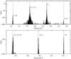 |
Fig. 7. LS periodograms. The main frequency f2 and its sidebands are shown in the top panel, and the higher harmonic frequency 2f2 and its sidebands are shown in the bottom panel. |
Figure 8 shows changes in modulation during the observation. The empty blocks for f0 correspond to portions of the light curve in which the double peak in the LS periodogram was present and an exact measurement was not possible, or the confidence of the peak is below 90% (see Table 1).
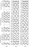 |
Fig. 8. Folded light curves of each portion. The first column is folded with frequency f0, the second with f1, and the third with f2. The empty plots for f0 refer to portions with a double peak, or to portions with a peak with a confidence level of < 90% (see Table 1). |
5. Discussion
The mini-outbursts occurred semi-regularly during the orbital period and for more than 16 years. These flares were peculiar in that they occur once per orbital period, at about the same orbital phase, and kept on recurring. This phenomenon is quite different from other bursting activity of larger amplitude observed in symbiotic stars (e.g., Gromadzki et al. 2013), which does not occur with such clear periodicity. We note that only AG Dra has flares with characteristics that are somewhat similar to those of FN Sgr (Gális et al. 2019), and in that case the flares recur with a typical period that is close to the pulsation of the red giant. However we do not have high-quality radial velocity data for FN Sgr with which we can detect such a pulsation.
The timescale and amplitude are similar to the first flaring event observed in the symbiotic system Z And, with an amplitude of 1.5 mag, a sharp rise, and a decay over ≈300 days (Sokoloski & Bildsten 1999). However, in Z And and other systems with repeated flares (e.g., AX Per, CI Cyg, BF Cyg), the recurrence times were always shorter than the orbital period, usually by about 10%–20% (see e.g., discussion in Mikolajewska 1996, 2002). A new outburst in Z And had a larger amplitude (2 mag) and lasted longer, and three separate flare episodes were observed over almost 3 years. Sokoloski et al. (2006) attributed this phenomenon outburst to a ‘combination nova’, namely nuclear shell burning triggered by a disc instability (Sokoloski et al. 2006). Another interesting finding is that the secondary period of ≃355 days found in the radial velocity data of the giant in Z And – which was attributed to the rotation of the giant (Gális et al. 1999; Friedjung et al. 2003) – is close to the recurrence semi-period of the outburst. A combination nova has also been invoked to explain the unusual recent outburst of a CV-like system, V1047 Cen (Aydi et al. 2022). We also note that, in Z And, a stable oscillation with a 28 min period was detected before and during the flare, which Sokoloski & Bildsten (1999) attributed to the rotation of a magnetic WD (with B ≥ 105 Gauss).
The high-cadence Kepler light curve of FN Sgr over 81 days at the end of 2015 offers new clues but also new ‘puzzles’. We find a complex periodogram with a low frequency f0, and a group of higher frequencies (f1, f2 and other sidebands), which are reminiscent of the short-orbital-period WD binaries classified as intermediate polars (IPs), where the lower frequency is the orbital frequency of the binary, and the higher frequencies are mainly due to the WD spin and the beating between the spin and the orbital frequency (see e.g., Ferrario & Wickramasinghe 1999). Other sidebands with higher harmonics can also be present in IPs. By analogy, we suggest that the f2 frequency, which is stable, is likely to be due to the WD rotation. The WD spin frequency in IPs is observable because the polar caps are heated by magnetic accretion funneled to the poles by the magnetic field. Even if an accretion disc is formed, it is disrupted at the magnetospheric radius.
Sokoloski & Bildsten (1999) analysed the high-resolution photometry taken in 1998 of the FN Sgr and detected a possible variability in the frequency range of 25.5 − 900 d−1. Even if the uncertainty is very large, our frequency f1 agrees with this detection, indicating that the spin rotation was also observable in 1998.
While in IPs there is often a third frequency corresponding to the beat between the orbital and the rotational period, for FN Sgr, the f1 frequency is the beat between the proposed rotation frequency and the f0 frequency, which is generated by a structure that is not synchronised with the orbital motion. This structure is likely to be around the WD and to be illuminated by the WD as it rotates. Both f0 and f1 are unstable frequencies, and this is consistent with f1 being the beat, because if f0 is unstable, the beating must be unstable too.
The non-stability or quasi-periodicity of f0 is an important characteristic when studying a physical model. In the periodograms of IPs, either the WD spin frequency or the beating frequency is dominant (Ferrario & Wickramasinghe 1999). The beat is usually detected when there is an accretion disc, even if it is disrupted at a certain radius, namely in IPs and not in polars. Moreover, the WD rotation in polars, which accrete directly via the magnetic stream, tends to be synchronized. We propose two possible explanations for the f0 frequency, both of which imply the presence of a ‘structure’ or a denser element in the accretion disc. If this element has negligible mass compared with the WD, and orbits a WD of 0.7 M⊙ (Brandi et al. 2005) with Keplerian angular velocity derived from the period associated with f0 (≈135.5 min), it must be localised in the very inner disc at ≃0.76 R⊙ from the centre.
One scenario is that the structure in the disc is not fixed, but is due to rocky detritus captured in the accretion disc around the WD. This would of course explain why the period is not perfectly stable. Rocky detritus has so far only been detected in 1 out of 3000 WDs, and is therefore a relatively rare phenomenon (see Vanderburg et al. 2020). We also examined the possibility of a ‘dark spot’, as in Kilic et al. (2015), although the event observed by these latter authors was recurrent with the period of the WD rotation.
Another possibility is that there is a vertical thickening of the accretion disc causing variable irradiation and inhomogeneities in the disc itself. In dwarf novae, the observed quasi-periodic oscillations (QPOs) may be caused by a vertical thickening of the disc, which moves as a travelling wave near the inner edge of the disc, alternately obscuring and reflecting radiation from the disc (Woudt & Warner 2002; Warner & Woudt 2002). Applied to FN Sgr, this model means that irradiation by the rotating WD would cause the QPO with beat frequency f1. However, the QPOs in dwarf novae have semi-periods of hundreds of seconds (e.g., Woudt & Warner 2003) and in FN Sgr the much longer period would imply inhomogeneities considerably farther from the disc centre compared to dwarf novae. In the model by Warner & Woudt (2002), the winding up and reconnection of magnetic field lines causes inhomogeneities. The magnetic field responsible for the phenomenon may be either that of the WD or that of an equatorial belt on the WD surface (low-inertia magnetic accretor model, Warner & Woudt 2002). As the inner disc radius where the inhomogeneities form depends on the magnetic field strength, the magnetic field of the WD in FN Sgr would be stronger than those of dwarf novae. This is consistent with magnetically channelled accretion, which allows detection of the rotation period.
5.1. The possibility of rocky bodies around the WD
Recent Kepler photometry has revealed that WDs display periodic optical variations that are very similar to the detected 2.2 h periodicity found in FN Sgr. Maoz et al. (2015) analysed Kepler light curves of 14 hot WDs and detected periodic variations with periodicities from 2 h to 10 days. Possible explanations include transits of objects of ∼50–200 km in dimension. The periodicity may arise from UV metal-line opacity due to the accretion of rocky material, such as debris from former planetary systems, a phenomenon observed in many WDs (e.g., Jura 2003; Zuckerman et al. 2003, 2010; Vanderburg et al. 2015; Xu et al. 2018; Vanderbosch et al. 2021). WD 2359−434, for instance, shows variability with a period of 2.7 h (Gary et al. 2013).
Some of the characteristics observed for rocky detritus so far differ significantly from what we detected in FN Sgr:
-
The quasi-periodic signals change in shape and amplitude quite significantly over the course of tens of days, while in FN Sgr the changes in amplitude and phase observed over 81 days were much smaller.
-
The shape of the dip is very sharp and asymmetric. We also note that, in WD 1145+017 b, for example, the small exoplanet orbiting the WD causes a very sharp feature in the light curve (Vanderburg et al. 2015; Gänsicke et al. 2016).
-
There are multiple periodic signals with similar periods.
-
The typical timescales of the features observed in the light curves are around 1 min only.
Therefore, the dips in luminosity caused by the detritus seem to always be sharp, short in duration, and variable; and often there are multiple periods. Looking at these characteristics, we conclude that our observations do not match the rocky detritus scenario, and that this possibility is relatively unlikely.
5.2. Interpretation as inhomogeneity in the accretion disc
Disc inhomogeneities can be generated by the stream–disc overflow, causing vertical disc thickening, as in GU Mus (Peris et al. 2015). These inhomogeneities may liberate blobs of matter rotating with Keplerian angular velocity at the radius where the vertical thickening occurs. However, in GU Mus the stream overflow generates the thickening at the circularisation radius6, which in FN Sgr is approximately 35.2 R⊙, while we infer a distance of only 0.76 R⊙ from the centre.
Lubow & Shu (1975) estimated the minimum distance of the stream from the centre to be
 (1)
(1)
where a is the binary separation and q is the binary mass ratio (donor mass divided by the WD). The minimum distance in FN Sgr is therefore 11.8 R⊙.
These estimates are based on the assumption of a Keplerian disc, but Brandi et al. (2005) suggested that the disc around the WD is geometrically thick. This may suggest that in FN Sgr there is a sub-Keplerian advection-dominated disc, meaning that the radial velocity of the matter is much larger than in a thin disc (Narayan & Yi 1994). The frequency f0 in thick discs is defined as η/(2π) ΩK, where η is the sub-Keplerian factor between approximately 0.2 and 1 (middle panel of Fig. 1 in Narayan & Yi 1994). The structure or inhomogeneity therefore does not need to be located as far from the WD as in the Keplerian, thin disc case.
While the spin and beat modulations have almost sinusoidal shapes, the QPOs with frequency f0 have a steep rise and slow dissipation (Fig. 8). Such asymmetry can be understood as rapid generation of the inhomogeneity, followed by its slow dissipation while orbiting the WD.
We note that, while f2 is clearly detected in almost all subsamples, the beating frequency f1 is only strong in the first half of the light curve (Fig. 6). If the beat is caused by a body rotating around the WD, the weak power implies that this body is not well irradiated by the rotating WD in the second half of the light curve, or that the irradiated surface is no longer clearly visible, supporting the idea that this body forms and dissipates slowly during the rotation around the WD.
As the duration of the light curve is 81 days, the angle of view changed by 0.1428 of the orbital cycle (51.4 deg). The clear visibility of the f1 frequency during the first half of the light curve suggests that a change of 0.0714 of the orbital cycle (25.7 deg) modifies the angle of view in such a way that the beating region no longer clearly shows the irradiated part. Our Kepler observation started approximately 29 days before the superior conjunction of the red giant (Fig. 2), which is 0.0511 of the orbital cycle (≈18.4 deg). After half of the observation (25.7 deg), f1 becomes weaker. Figure 9 shows a model of this configuration. The line with angle −18.4° represents the viewing angle at the start of the Kepler observation, while 7.3° is half of the observation, where f1 becomes significantly weaker.
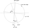 |
Fig. 9. Schematic illustration of the angle of view during the Kepler observation. The line marked with angle 0° points towards the giant or L1. The other angles represent the beginning (−18.4°) and the middle (7.3°) in the Kepler observation. The inner disc edge is marked as a circle with an arrow showing the sense of rotation. The small circle represents the region where the inhomogeneity blobs may be originating (see text for details). ϕ denotes the orbital phase and corresponding viewing angle. |
The f1 variability starts to decline at the viewing angle of 7.3°. Therefore, if we suppose that there are inhomogeneous blobs visible up to 90° from the viewing direction, the small circle in Fig. 9 shows the regions where these blobs are generated. After sweeping this region, the blobs are not visible enough or dissipate slowly and become too small to generate a strong beat. Following Lubow & Shu (1975, 1976), the region of blob generation can be associated with the stream–disc overflow or simply with the trajectory from the L1 point. Stream–disc overflow requires a thin-disc geometry, while if the disc is geometrically thick, there is not an actual overflow of the accretion stream, but from the point L1, the stream may impinge the disc, penetrate it, and generate blobs at its inner edge.
5.3. The mini-outbursts
As the outbursts seem to be almost phase-locked, an episodic mass-accretion rate would be a plausible interpretation. An eccentric orbit could cause mass-accretion events when the secondary approaches the primary WD. However, Brandi et al. (2005) concluded that the orbit is almost circular.
An alternative explanation, based on a phased-locked behaviour, is that a bright region appears at specific viewing angles. Figure 9 shows the viewing angles of phases 0.3 and 0.5. The mini-outburst ends at approximately phase 0.5, which is very close to the viewing angle where the f1 frequency starts to disappear. This implies a related physical origin of the two events, and the mini-outburst should be connected to the stream–disc overflow or to the stream–disc impact region.
Although the stream–disc scenario appears to be a plausible explanation, we investigated several other possibilities. An explanation in terms of thermonuclear runaway (a recurrent ‘non-ejecting nova’ as in Yaron et al. (2005) implies an accretion rate of the order of 10−6 M⊙ yr−1 and a recurrence time that would decrease from ≃10 years to ≃2 years for increasing WD mass from 0.65 to 1 M⊙ (Yaron et al. 2005). However, such an outburst would cause an increase by ≃4 mag in V.
A third possibility is that the outbursts are related to the magnetic field. In the old nova and IP GK Per, with an orbital period of almost 2 days and a subgiant K2 secondary, dwarf-nova-like-outbursts with a recurrence time of 400±40 days and amplitude of 1–3 mag have been observed for decades (see Zemko et al. 2017, and references therein). Although the exact mechanism powering these outbursts is a matter of debate, it seems certain that the maximum temperature of the disc and therefore its inner radius decrease in outburst, and more matter is suddenly accreted (Zemko et al. 2017). The timescale of the FN Sgr mini-flares is similar, although the much higher luminosity of the system and the larger orbit make it difficult to draw a comparison.
Assuming that the WD is strongly magnetised (B ≥ 105 Gauss), as indicated by our Kepler timing analysis, there are two further, alternative explanations. The magnetosphere may cause ‘magnetically gated accretion’ (Scaringi et al. 2017): unstable, magnetically regulated accretion causing quasi-periodic bursts. In this model, the disc material builds up around the magnetospheric boundary and, reaching a critical amount, the matter accretes onto the WD, causing an optical flare. Scaringi et al. (2017) studied this phenomenon in the cataclysmic variable MV Lyr, where quasi-periodic bursts of ∼30 min appeared every ∼2 h. The main question is how the timescale would vary in a symbiotic star, that is, a binary with a much longer orbital period.
The recurrence time of these bursts is typically close to the viscous timescale tvisc in the region where the instability occurs (inner disc):
 (2)
(2)
where rin is the inner disc radius and ν is a viscosity parameter. Assuming that the magnetospheric radius is 0.76 R⊙ (derived in the previous section), and with the viscosity parameter expressed in terms of dimensionless α parameter following Shakura & Sunyaev (1973),
 (3)
(3)
where h/r is the ratio of the scale height h of the disc at radial distance r, G is the gravitational constant, and mWD is the WD mass. The mini-outbursts seem to be almost phase locked, and therefore tvisc would have to be close to the orbital period of 567.3 days. If the disc is geometrically thick, with h/r = 0.1, the observed recurrence time of FN Sgr is obtained only with α = 0.0026. However, we know that a realistic value of 0.1 for α in advective discs (Narayan & Yi 1994) yields a much larger magnetospheric radius, namely 8.7 R⊙. Moreover, the h/r ratio may even be as high as 0.4 (e.g., Godon 1996), shortening tvisc considerably. On the basis of these considerations, we rule this model out.
An interesting possibility that we would like to consider is that of a localised thermonuclear runaway (LTNR), namely a thermonuclear runaway that does not spread over the entire surface, as in helium burning on neutron stars. Shara (1982) proposed that dwarf-nova-like, ‘volcanic’ eruptions of small amplitude occur on the surface of massive WDs and may recur on timescales of months due to LTNRs. In the model proposed by these latter authors, the eruption causes a sort of volcano to reach the WDs surface, without mass ejection. Orio & Shaviv (1993) modelled the LTNR with the formalism used for helium burning on neutron stars and calculated that temperature differences as small as 104–105 K at the bottom of the envelope accreted by a WD can lead to a LTNR that remains confined and is extinguished before spreading over the entire surface. If accretion funneled by the magnetic field to the WD poles produces such a temperature gradient, a LTNR may occur. The higher the WD mass and the larger the mass-accretion rate, the more likely it is that a LTNR will occur. The LTNR may remain confined only for a certain time; if it is not extinguished, it will later spread over the entire surface, causing a classical nova with a slow rise (a day or more).
The LTNR scenario has recently been revisited. A LTNR model involving the magnetic field was studied for highly magnetised WDs, B > 106 G, in order to explain very small-amplitude flashes recently observed in CVs, referred to as micronovae by the authors (Scaringi et al. 2022a,b). Such flashes cause luminosity increases of a few to ≃30 times occurring within hours and recurring on timescales of months. The strength of the magnetic field that allows accretion to be confined to a region at the poles is estimated assuming the inner radius of an accretion disc truncated by the magnetosphere because of magnetic pressure balancing the ram pressure of the accretion flow. This defines a magnetospheric radius (see e.g., Frank et al. 1992)
 (4)
(4)
where ṁacc is the mass-accretion rate, m1 is the WD mass, and  is the magnetic moment of the WD.
Figure 10 shows B values calculated for various mass-accretion rates. We assumed 0.76 R⊙ for the truncation radius rm. The most likely radius of the 0.7 M⊙ WD is R1 = 0.013 R⊙ (from the mass–radius relation by Nauenberg 1972). The WD radius may be larger if the WD atmosphere is inflated, but this usually occurs because of hydrogen burning over the entire surface (see Starrfield et al. 2012). We take into account the possibility of a larger WD radius in Fig. 10. However, we note two issues: (a) an apparent typo in Brandi et al. (2005), as from the values in their Table 5, namely a hot, hydrogen-burning WD with Teff = 150 000–180 000 K and L ≃ 1000–2000 L⊙ should have a radius of around R2 ≃ 0.02 R⊙ instead of 0.2 R⊙; and (b) if nuclear burning is localised, the large UV luminosity should be ascribed to the accretion disc and not to the WD. In any case, we take into account the possibility of a larger WD radius in Fig. 10.
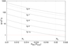 |
Fig. 10. WD magnetic field calculated using Eq. (4) for different values of the mass-accretion rate. The solid lines trace the solution with the magnetospheric radius of 0.76 R⊙, and mass-accretion rates from 10−6 to 10−10 M⊙ yr−1 (marked as labels). The dashed line represents the solution with a magnetospheric radius of 0.6 R⊙ and a mass-accretion rate of 10−6 M⊙ yr−1. The horizontal red line is traced at the magnetic field of B = 106 G. The vertical dotted lines represent two WD radii: R1 = 0.013 R⊙ and R2 = 0.02 R⊙ (see text for details). |
Allowing for a radius of R2 ≃ 0.02 R⊙, the micronova scenario is acceptable with a magnetic field higher than a few megaGauss and with ṁ of a few 10−10 M⊙ yr−1. However, for values of ṁ that are closer to what has been inferred in many symbiotic stars, the magnetic field should be of at least the order of hundreds of megaGauss, which is unusual for WDs. If the matter orbits more slowly than the Keplerian velocity because of the geometrically thick disc, the inner disc radius can be smaller, but this would only slightly affect the result, as shown by the dashed line in Fig. 10.
A detection in supersoft X-rays would be extremely useful, and would allow us to understand whether or not the WD atmospheric temperature and bolometric luminosity are as high as those derived by Brandi et al. (2005); if they are, the burning is unlikely to be localised. However, highly stringent upper limits on the bolometric luminosity may be difficult to obtain given the distance and the possible large intrinsic absorption in the symbiotic nebula.
6. Summary and conclusions
The V and I light curves observed over decades reveal that for many years, from before 2001 until 2019, the symbiotic system FN Sgr underwent recurrent optical flares with amplitudes of 0.5–1 mag, at orbital phases 0.3–0.5, with a sharp rise over 10 days and a decay lasting many weeks. The amplitude and timescales of the outbursts cannot be explained with a disc instability triggered by a burst of mass transfer, with a non-ejecting thermonuclear flash, nor with a combination nova. Given the detection of a likely rotation period in the Kepler light curve, we find that the WD is likely to have a strong magnetic field, ≥105 Gauss. We examined two alternatives recently proposed for small-amplitude flares of magnetic cataclysmic variables, and how they may be relevant for a symbiotic system with a magnetic WD. A thermonuclear runaway in a ‘non-ejecting nova’ would occult with a higher luminosity amplitude than observed in FN Sgr. We find that localised thermonuclear burning confined by the magnetic field may explain the observed phenomena with B ≥ 106 Gauss and an accretion rate of ≥10−10 M⊙ yr−1. However, localised burning is difficult to reconcile with the high bolometric luminosity and temperature of the ionising source inferred from the UV range and from the flux of the He II λ 4686 emission line by Brandi et al. (2005). If the WD is indeed the ionising source, as suggested by the above authors, it is so hot and luminous that thermonuclear burning must be ongoing over the entire surface.
An interesting comparison can be made with the periodic outbursts of the IP and old nova GK Per. However, the difference in luminosity and spatial dimensions make a rigorous comparison very difficult.
The most promising interpretation is based on the phase-locked appearance of the mini-outbursts. This points to the visibility of the stream–disc overflow, which also coincides with conclusions derived from our detailed timing analysis.
The Kepler timing analysis revealed three dominant frequencies with sidebands. The lowest frequency f0 is unstable and probably represents an inhomogeneity generated at the inner disc edge. The higher frequency f2 (11.3 min periodicity) is very stable and we attribute it to a magnetic rotating WD. We also measured a frequency f1, corresponding to the beating between f1 and f2.
The f0 and f2 frequencies are present during the whole light curve, suggesting permanent visibility of the corresponding sources. The stability of f2 is consistent with the idea that it is the frequency generated by the rotating WD. We interpret f0 as a frequency generated by an inner disc inhomogeneity, indicating the presence of blobs or rigid bodies during the whole orbital period. The shape of the folded light curve implies that these may be blobs that form and dissipate slowly. The beat frequency f1 is only strong during the first half of the observation. This is consistent with the region of strongest irradiation of the blobs being associated with the trajectory of an accretion stream from the point L1, impinging the geometrically thick disc of FN Sgr, penetrating it, and generating inhomogeneity blobs at the inner disc edge.
We examined an alternative explanation for the f1 frequency, namely rocky detritus around the WD, but the characteristics of the modulation are very different from what has been observed so far in nearby WDs.
MJD = JD – 2400000.
The Kepler team evaluates the contribution of scattered background light and subtracts it at the pixel level. The background is a large source of photon noise. For faint stars, where the background is much larger than the star flux, the estimated brightness may be negative.
Python hampel library https://github.com/MichaelisTrofficus/hampelfilter
SciPy Python’s package https://scipy.org/
Astropy Python’s package https://docs.astropy.org/en/stable/index.html was calculated with normalization set to “standard”.
The circularisation radius is the distance from the centre where angular momentum from the L1 point is equal to the local specific angular momentum of a Keplerian disc.
Acknowledgments
JMag, AD, and PB were supported by the European Regional Development Fund, project No. ITMS2014+: 313011W085. JMik was supported by the Polish National Science Centre (NCN) grant OPUS 2017/27/B/ST9/01940.
References
- Aydi, E., Sokolovsky, K. V., Bright, J. S., et al. 2022, ApJ, 939, 6 [NASA ADS] [CrossRef] [Google Scholar]
- Barba, R., Brandi, E., Garcia, L., & Ferrer, O. 1992, PASP, 104, 330 [NASA ADS] [CrossRef] [Google Scholar]
- Brandi, E., Mikołajewska, J., Quiroga, C., et al. 2005, A&A, 440, 239 [NASA ADS] [CrossRef] [EDP Sciences] [Google Scholar]
- Ferrario, L., & Wickramasinghe, D. T. 1999, MNRAS, 309, 517 [NASA ADS] [CrossRef] [Google Scholar]
- Frank, J., King, A., & Raine, D. 1992, Accretion Power in Astrophysics (Cambridge: Cambridge University Press), 21 [Google Scholar]
- Friedjung, M., Gális, R., Hric, L., & Petrík, K. 2003, A&A, 400, 595 [NASA ADS] [CrossRef] [EDP Sciences] [Google Scholar]
- Gális, R., Hric, L., Friedjung, M., & Petrík, K. 1999, A&A, 348, 533 [Google Scholar]
- Gális, R., Merc, J., Leedjärv, L., Vrašťák, M., & Karpov, S. 2019, Open Eur. J. Variable Stars, 197, 15 [Google Scholar]
- Gänsicke, B. T., Aungwerojwit, A., Marsh, T. R., et al. 2016, ApJ, 818, L7 [CrossRef] [Google Scholar]
- Gary, B. L., Tan, T. G., Curtis, I., Tristram, P. J., & Fukui, A. 2013, Soc. Astron. Sci. Ann. Symp., 32, 71 [NASA ADS] [Google Scholar]
- Godon, P. 1996, ApJ, 462, 456 [NASA ADS] [CrossRef] [Google Scholar]
- Gromadzki, M., Mikołajewska, J., & Soszyński, I. 2013, Acta Astron., 63, 405 [NASA ADS] [Google Scholar]
- Jura, M. 2003, ApJ, 584, L91 [Google Scholar]
- Kilic, M., Gianninas, A., Bell, K. J., et al. 2015, ApJ, 814, L31 [NASA ADS] [CrossRef] [Google Scholar]
- Lubow, S. H., & Shu, F. H. 1975, ApJ, 198, 383 [NASA ADS] [CrossRef] [Google Scholar]
- Lubow, S. H., & Shu, F. H. 1976, ApJ, 207, L53 [NASA ADS] [CrossRef] [Google Scholar]
- Maoz, D., Mazeh, T., & McQuillan, A. 2015, MNRAS, 447, 1749 [NASA ADS] [CrossRef] [Google Scholar]
- Mikolajewska, J. 1996, in IAU Colloq. 158: Cataclysmic Variables and Related Objects, eds. A. Evans, & J. H. Wood, Astrophys. Space Sci. Lib., 208, 335 [NASA ADS] [CrossRef] [Google Scholar]
- Mikolajewska, J. 2002, A&A, 392, 197 [NASA ADS] [CrossRef] [EDP Sciences] [Google Scholar]
- Mikołajewska, J. 2012, Balt. Astron., 21, 5 [NASA ADS] [Google Scholar]
- Munari, U., & Buson, L. M. 1994, A&A, 287, 87 [NASA ADS] [Google Scholar]
- Narayan, R., & Yi, I. 1994, ApJ, 428, L13 [Google Scholar]
- Nauenberg, M. 1972, ApJ, 175, 417 [NASA ADS] [CrossRef] [Google Scholar]
- Orio, M., & Shaviv, G. 1993, Ap&SS, 202, 273 [NASA ADS] [CrossRef] [Google Scholar]
- Peris, C. S., Vrtilek, S. D., Steiner, J. F., et al. 2015, MNRAS, 449, 1584 [CrossRef] [Google Scholar]
- Scargle, J. D. 1982, ApJ, 263, 835 [Google Scholar]
- Scaringi, S., Maccarone, T. J., D’Angelo, C., Knigge, C., & Groot, P. J. 2017, Nature, 552, 210 [NASA ADS] [CrossRef] [Google Scholar]
- Scaringi, S., Groot, P. J., Knigge, C., et al. 2022a, Nature, 604, 447 [NASA ADS] [CrossRef] [Google Scholar]
- Scaringi, S., Groot, P. J., Knigge, C., et al. 2022b, MNRAS, 514, L11 [NASA ADS] [CrossRef] [Google Scholar]
- Shakura, N. I., & Sunyaev, R. A. 1973, A&A, 24, 337 [NASA ADS] [Google Scholar]
- Shara, M. M. 1982, ApJ, 261, 649 [NASA ADS] [CrossRef] [Google Scholar]
- Sokoloski, J. L., & Bildsten, L. 1999, ApJ, 517, 919 [NASA ADS] [CrossRef] [Google Scholar]
- Sokoloski, J. L., Kenyon, S. J., Espey, B. R., et al. 2006, ApJ, 636, 1002 [NASA ADS] [CrossRef] [Google Scholar]
- Starrfield, S., Iliadis, C., Timmes, F. X., et al. 2012, Bull. Astron. Soc. India, 40, 419 [NASA ADS] [Google Scholar]
- Vanderbosch, Z. P., Rappaport, S., Guidry, J. A., et al. 2021, ApJ, 917, 41 [NASA ADS] [CrossRef] [Google Scholar]
- Vanderburg, A., & Johnson, J. A. 2014, PASP, 126, 948 [Google Scholar]
- Vanderburg, A., Johnson, J. A., Rappaport, S., et al. 2015, Nature, 526, 546 [Google Scholar]
- Vanderburg, A., Latham, D. W., Buchhave, L. A., et al. 2016, ApJS, 222, 14 [Google Scholar]
- Vanderburg, A., Rappaport, S. A., Xu, S., et al. 2020, Nature, 585, 363 [Google Scholar]
- Warner, B., & Woudt, P. A. 2002, MNRAS, 335, 84 [NASA ADS] [CrossRef] [Google Scholar]
- Woudt, P. A., & Warner, B. 2002, MNRAS, 333, 411 [NASA ADS] [CrossRef] [Google Scholar]
- Woudt, P. A., & Warner, B. 2003, MNRAS, 340, 1011 [NASA ADS] [CrossRef] [Google Scholar]
- Xu, S., Rappaport, S., van Lieshout, R., et al. 2018, MNRAS, 474, 4795 [Google Scholar]
- Yaron, O., Prialnik, D., Shara, M. M., & Kovetz, A. 2005, ApJ, 623, 398 [Google Scholar]
- Zemko, P., Orio, M., Luna, G. J. M., et al. 2017, MNRAS, 469, 476 [NASA ADS] [CrossRef] [Google Scholar]
- Zuckerman, B., Koester, D., Reid, I. N., & Hünsch, M. 2003, ApJ, 596, 477 [Google Scholar]
- Zuckerman, B., Melis, C., Klein, B., Koester, D., & Jura, M. 2010, ApJ, 722, 725 [Google Scholar]
All Tables
All Figures
|
Fig. 1. Optical light curve of FN Sgr. Data from (Brandi et al. 2005) are shown in black, the ASAS data in green, and our new data in blue. The Kepler light curve is also shown in red, offset vertically by 12 mag for comparison with the V-band data. |
| In the text | |
|
Fig. 2. Kepler light curve (red points) with optical data from Fig. 1. The red dashed line shows the superior conjunction of the red giant. |
| In the text | |
|
Fig. 3. Selected time interval of V light curve from Fig. 1, and corresponding V − I index. The blue and red dashed lines correspond to the inferior and superior conjunction of the red giant, respectively. The blue thick dashed line is the reference optical minimum determined by polynomial fitting. |
| In the text | |
|
Fig. 4. LS periodogram with power in logarithmic scale. The red dashed line indicates the 90% confidence level. |
| In the text | |
|
Fig. 5. Peak pattern of the f0, f1, and f2 frequencies given by the LS periodogram. |
| In the text | |
|
Fig. 6. LS periodogram per portion, obtained by dividing the Kepler light curve into 20 equally spaced sub-samples. The first column represents f0, the second f1, and the third f2. The vertical lines indicate the mean value of f1 and f2, or Δ when f0 was computed as the difference between the two frequencies. |
| In the text | |
|
Fig. 7. LS periodograms. The main frequency f2 and its sidebands are shown in the top panel, and the higher harmonic frequency 2f2 and its sidebands are shown in the bottom panel. |
| In the text | |
|
Fig. 8. Folded light curves of each portion. The first column is folded with frequency f0, the second with f1, and the third with f2. The empty plots for f0 refer to portions with a double peak, or to portions with a peak with a confidence level of < 90% (see Table 1). |
| In the text | |
|
Fig. 9. Schematic illustration of the angle of view during the Kepler observation. The line marked with angle 0° points towards the giant or L1. The other angles represent the beginning (−18.4°) and the middle (7.3°) in the Kepler observation. The inner disc edge is marked as a circle with an arrow showing the sense of rotation. The small circle represents the region where the inhomogeneity blobs may be originating (see text for details). ϕ denotes the orbital phase and corresponding viewing angle. |
| In the text | |
|
Fig. 10. WD magnetic field calculated using Eq. (4) for different values of the mass-accretion rate. The solid lines trace the solution with the magnetospheric radius of 0.76 R⊙, and mass-accretion rates from 10−6 to 10−10 M⊙ yr−1 (marked as labels). The dashed line represents the solution with a magnetospheric radius of 0.6 R⊙ and a mass-accretion rate of 10−6 M⊙ yr−1. The horizontal red line is traced at the magnetic field of B = 106 G. The vertical dotted lines represent two WD radii: R1 = 0.013 R⊙ and R2 = 0.02 R⊙ (see text for details). |
| In the text | |
Current usage metrics show cumulative count of Article Views (full-text article views including HTML views, PDF and ePub downloads, according to the available data) and Abstracts Views on Vision4Press platform.
Data correspond to usage on the plateform after 2015. The current usage metrics is available 48-96 hours after online publication and is updated daily on week days.
Initial download of the metrics may take a while.