| Issue |
A&A
Volume 675, July 2023
|
|
|---|---|---|
| Article Number | A55 | |
| Number of page(s) | 14 | |
| Section | The Sun and the Heliosphere | |
| DOI | https://doi.org/10.1051/0004-6361/202245611 | |
| Published online | 30 June 2023 | |
Interchange reconnection dynamics in a solar coronal pseudo-streamer⋆
1
Sorbonne Université, École polytechnique, Institut Polytechnique de Paris, Université Paris Saclay, Observatoire de Paris, Université PSL, CNRS, Laboratoire de Physique des Plasmas (LPP), Paris, France
e-mail: This email address is being protected from spambots. You need JavaScript enabled to view it.
2
Observatoire Radioastronomique de Nançay, Observatoire de Paris, CNRS, PSL, Université d’Orléans, Nançay, France
3
Department of Mathematical Sciences, Durham University, Durham, DH1 3LE
UK
4
Heliophysics Science Division, NASA Goddard Space Flight Center, Greenbelt, MD 20771
USA
Received:
2
December
2022
Accepted:
25
April
2023
Abstract
Context. The generation of the slow solar wind remains an open problem in heliophysics. One of the current theories among those aimed at explaining the injection of coronal plasma in the interplanetary medium is based on interchange reconnection. It assumes that the exchange of magnetic connectivity between closed and open fields allows the injection of coronal plasma in the interplanetary medium to travel along the newly reconnected open field. However, the exact mechanism underlying this effect is still poorly understood.
Aims. Our objective is to study this scenario in a particular magnetic structure of the solar corona: a pseudo-streamer. This topological structure lies at the interface between open and closed magnetic field and is thought to be involved in the generation of the slow solar wind.
Methods. We performed innovative 3D magnetohydrodynamic (MHD) simulations of the solar corona with a pseudo-streamer, using the Adaptively Refined MHD Solver (ARMS). By perturbing the quasi-steady ambient state with a simple photospheric, large-scale velocity flow, we were able to generate a complex dynamics of the open-and-closed boundary of the pseudo-streamer. We studied the evolution of the connectivity of numerous field lines to understand its precise dynamics.
Results. We witnessed different scenarios of opening of the magnetic field initially closed under the pseudo-streamer: one-step interchange reconnection dynamics, along with more complex scenarios, including a coupling between pseudo-streamer and helmet streamer, as well as back-and-forth reconnections between open and closed connectivity domains. Finally, our analysis revealed large-scale motions of a newly opened magnetic field high in the corona that may be explained by slipping reconnection.
Conclusions. By introducing a new analysis method for the magnetic connectivity evolution based on distinct closed-field domains, this study provides an understanding of the precise dynamics underway during the opening of a closed field, which enables the injection of closed-field, coronal plasma in the interplanetary medium. Further studies shall provide synthetic observations for these diverse outgoing flows, which could be measured by Parker Solar Probe and Solar Orbiter.
Key words: magnetic fields / Sun: corona / magnetohydrodynamics (MHD) / magnetic reconnection / solar wind
Movies associated to Figs. 9–13 are available at https://www.aanda.org.
© The Authors 2023
 Open Access article, published by EDP Sciences, under the terms of the Creative Commons Attribution License (https://creativecommons.org/licenses/by/4.0), which permits unrestricted use, distribution, and reproduction in any medium, provided the original work is properly cited.
This article is published in open access under the Subscribe to Open model. This email address is being protected from spambots. You need JavaScript enabled to view it. to support open access publication.
1. Introduction
As is the case for many stars, the Sun generates a plasma flow, known as the solar wind, that constitutes its heliosphere. It is generally acknowledged that during solar minimum, the solar wind has two regimes: a fast wind coming from the pole and a slow wind originating from low latitude regions (roughly 60° wide around the Sun’s equatorial plane; Wang 2000; McComas et al. 2008). In addition to its mean velocity, the slow solar wind differs from the fast solar wind by its composition, a higher heavy-ion ionization state, and a higher first ionization potential bias in elemental abundances, as well as a greater temporal variability (see reviews by Schwenn 2006; Geiss et al. 1995; von Steiger et al. 2000; von Steiger & Zurbuchen 2011).
While coronal holes (CHs) are widely accepted as the source region of the fast wind, the source of the slow wind is still a matter of intense debate (see review by Abbo et al. 2016). Several coronal models have been proposed to explain the slow solar wind properties. The expansion factor model provides an empirical relation between the speed of the wind and the expansion factor of the open magnetic field in coronal holes (Wang & Sheeley 1990). Assuming that the heating rate depends on the local magnitude of the coronal hole magnetic field, when the magnetic field diverges rapidly with height, most of the energy is deposited in the low corona (Wang et al. 2009). There is less energy available for the plasma flow on the edges of the coronal holes where the field is diverging faster than in their core. Thus, slow wind originates from the CH edge (large expansion factor), while the fast wind comes from the CH core (small expansion factor). Pinto et al. (2016) tested this model using numerical magnetohydrodynamics (MHD) simulation and highlighted that the expansion factor strongly depends on the topology of the magnetic field. A major issue related to the expansion factor model lies in its inability to explain the slow-wind composition and variability measured in the heliosphere.
In order to explain the slow solar wind variability, dynamical models have been developed, such as the streamer blob model and the interchange reconnection model. The streamer blob model (see Sheeley et al. 1997; Higginson & Lynch 2018; Lynch 2020) relies on the creation of magnetic flux ropes by magnetic reconnection at the apex of the helmet streamer and may account for the slow wind speed and density variability (Viall & Vourlidas 2015). A flux rope can be formed by magnetic reconnection either between closed-closed field that have been extended by the solar wind and pinched at the top of the streamer (Higginson & Lynch 2018; Réville et al. 2020, 2022) or between open-open field on each side of the heliospheric current sheet (HCS). Independently of the reconnection type, the plasma blobs are released in the HCS localized around the Sun’s equator and cannot directly explain the presence of slow wind as much as 60° in latitude away from the ecliptic plane.
The interchange reconnection model proposed by Fisk et al. (1998) is aimed at explaining the variability of the slow wind by the release of hot plasma flows from closed-coronal loops that reconnect with the nearby open field (Del Zanna et al. 2011). Diverse topologies of the magnetic field are favorable to the development of interchange reconnection. Single 3D magnetic null point appears when a parasitic polarity is embedded in an opposite sign polarity which creates a (quasi-)circular polarity inversion line (PIL). When magnetic field surrounding the parasitic polarity is open, the fan separatrix surface of the null point presents a dome shape, which encloses a domain of closed magnetic field that is topologically separated from the surrounding open field. Two singular field lines originate from the null point on each side of the fan surface. One spine is anchored inside the parasitic polarity and the other one is open in the corona. Magnetic null points with open spines are widely known to serve as the playground for coronal jets injecting coronal plasma and energetic particles along the open field that is newly reconnected through interchange reconnection (Pariat et al. 2009; Rosdahl & Galsgaard 2010; Raouafi et al. 2016; Pallister et al. 2021). In order to have an open spine, the fan does not have to be entirely surrounded by open field, but the open field region has to be continuous; namely, the fan can be partially inserted into the open field region (Edmondson et al. 2010).
More recently, Titov et al. (2011) defined a more complex magnetic topology at the interface of open and closed fields in the corona, namely: pseudo-streamer (PS) topology. Pseudo-streamers were first identified as large-scale structures in EUV wavelengths (Wang & Sheeley 2007; Seaton et al. 2013). The underlying magnetic structure of a pseudo-streamer consists of a closed field embedded in uni-polar open field – unlike a helmet streamer, which is embedded in bipolar open field (Riley & Luhmann 2012; Rachmeler et al. 2014). Pseudo-streamers are usually located at higher latitudes than active regions and associated with decaying active regions (Rachmeler et al. 2014; Seaton et al. 2013). By analyzing the magnetic topology of the global coronal magnetic field, Titov et al. (2012) showed that multiple pseudo-streamers can be present concomitantly and that their topology altogether structures the large-scale corona. Similarly to null points with an open spine, pseudo-streamers are formed when a parasitic polarity is embedded in an opposite sign polarity, creating a quasi-circular PIL. However, the open field is distributed in two disconnected regions Scott et al. (2021). A pseudo-streamer topology displays a central null point with a vertical fan, which is called the separatrix curtain, and two spines that belong to the closed separatrix dome enclosing the parasitic polarity. The vertical fan is partially open. Its opened section delimits the two disconnected regions of open field, while two closed field sections are located on each side of the open section and belong to the closed field of the helmet streamer. The vertical fan intersects the two helmet streamer open-closed boundaries located on each side of the pseudo-streamer. We find open separators at those intersections. The closed separatrix dome of the pseudo-streamer is built by the two dome-shaped closed fans from two null points located on each side of the central null. Two spines of those secondary null points belong to the vertical fan of the central null. Also, the two null points can be located at the solar surface and thus form bald patches. We refer to Titov et al. (2011) for more details. The central null and the secondary nulls (or bald patches) are connected by separators formed at the intersection of the vertical fan and the closed-dome separatrix surfaces.
Magnetic reconnection happening at a separatrix surface leads to a change of magnetic connectivity domain of the reconnecting field. During the interchange reconnection, the closed field switch from the close connectivity domain below the closed separatrix surface toward the connectivity domain of open field. In the corona, a second type of topological element exists, namely, the quasi-separatrix layer or QSL. It defines a volume of strong gradient of magnetic connectivity: a magnetic flux highly concentrated at one footpoint strongly diverge and connect an extended and squashed area at its conjugate footpoint (Demoulin et al. 1996; Titov et al. 2002). QSLs are found in bipolar magnetic configuration (Demoulin et al. 1997; Mandrini 1997) and embed true separatrices (Masson et al. 2009; Pontin et al. 2016). Magnetic reconnection occurs in QSLs and leads to a continuous change of magnetic connectivity inside the QSLs (Aulanier et al. 2006). They are quantified by computing the squashing-factor Q which measures gradient of connectivity for each field line with respect to its neighboring field lines (Titov et al. 2002; Pariat & Démoulin 2012).
The separatrix-web model (S-Web) was proposed by Antiochos et al. (2011) and Linker et al. (2011) to explain the slow wind’s latitudinal extension away from the HCS, its variability, and its composition (charge-state and elemental). This model relies on the large-scale magnetic topology of the solar corona. By computing the squashing factor Q of the global coronal magnetic field between the solar surface and 10 R⊙, these authors showed that there is a connected network of high-Q arcs. This web extends up to 30° in latitude south and north of the HCS (see Fig. 7 Antiochos et al. 2011). Those high-Q arcs show the open-closed separatrices and the associated QSLs (Scott et al. 2018). The S-Web model proposes that interchange reconnection occurs along this network of separatrices and quasi-separatrix layers, allowing for the dynamical release of closed coronal plasma into the heliosphere. It is worth mentioning that the S-web itself shows many high-Q arcs connected to the HCS, thus highlighting the fact that pseudo-streamers and narrow corridor structures are ubiquitous in the corona (Scott et al. 2018).
In the corona, the arcs of high Q are of two types (see Scott et al. 2018). They can be the heliospheric trace of a narrow corridor of open field in the corona (Antiochos et al. 2011) or serve as a signature of a PS topology (Titov et al. 2011). Those two magnetic configuration are fundamentally different. The open-closed separatrix surface for a narrow corridor corresponds to the surface delimiting the streamer and the open field and no true magnetic null point is present. The Q arc consists solely of a quasi-separatrix layer, without an embedded separatrix inside. By forcing the open-closed boundary of such narrow corridor, Higginson et al. (2017a) showed that interchange reconnection occur and exchange the open and closed connectivity of the field at the narrow corridor boundaries.
The second type of magnetic configuration creating high-Q arcs is the PS topology. Such a magnetic topology provides key elements to trigger interchange reconnections. In a series of studies, Aslanyan et al. (2021, 2022) have studied the open-closed dynamics in a PS topology by forcing the system with super-granular photospheric flows applied at the open field boundaries and along the closed separatrix surface. They showed that on a global scale, magnetic reconnection occurs and that field rooted in the photospheric flows is able to reconnect and open into the heliosphere.
On the other hand, pseudo-streamers have multiples topological elements where interchange reconnection can happen. Therefore, magnetic reconnection at null points are not the only way by which the field can open. Masson et al. (2014) suggested that the field can open via at least two different scenarios: (1) a standard interchange reconnection at the null point between the closed field below the PS closed dome and the open field or (2) a two-step reconnection combining a closed-closed reconnection between the closed field below the PS closed dome and the closed field below the helmet streamer, followed by the opening of the field through interchange reconnection at the open separator between the helmet streamer closed field and the open field. However, those conclusion are only based on the topological analysis and no dynamical study has been carried out. Knowledge of the detailed dynamics of the field opening is critical to linking the in situ measurement with the remote observations (Parenti et al. 2021) and thereby understanding the source of the slow wind.
In this paper, we present a numerical study that is tailored to achieve a better understanding of the dynamics of the pseudo-streamer. In Sect. 2, we present our pseudo-streamer numerical model. In Sect. 3, we analyze the dynamics of the pseudo-streamer and determine the reconnection episodes leading to the opening or the closing of the magnetic field. Finally, in Sect. 4, we present our conclusions and discuss the heliospheric impact of the open-closed connectivity exchange in a pseudo-streamer.
2. Model description
In this section, we first present the MHD equations and the numerical domain (Sect. 2.1). Then, we detail the initial magnetic field (Sect. 2.2) and the pseudo-streamer topology at the initial time (Sect. 2.3). We also describe the atmosphere initialization and the relaxation phase required to reach a quasi-steady state (Sect. 2.4). Finally, we present the photospheric flow that forces and disturbs the system (Sect. 2.5).
2.1. MHD equations and the numerical domain
The simulations are performed using the Adaptively Refined Magneto-hydrodynamics Solver (ARMS; DeVore & Antiochos 2008) to solve the following ideal MHD equations in spherical coordinates:
 (1)
(1)
 (2)
(2)
 (3)
(3)
where ρ is the mass density, v the plasma velocity, μ the magnetic permeability in vacuum, B the magnetic field, P the pressure, and g = −G M⊙r/r3 the solar gravitational acceleration. We assume a fully ionized hydrogen plasma so that P = 2(ρ/mP)kBT with T the plasma temperature and mP as the proton mass. Because our concern is not to simulate the detailed thermodynamics of the heliospheric plasma, but the dynamics of the coronal magnetic field, we did not solve the energy equation and, instead, we imposed a constant, uniform temperature.
The ARMS code uses the PARAMESH toolkit (MacNeice et al. 2000) that provides parallel adaptive mesh refinement to adapt the grid throughout the computation to the evolving solution. Five levels of grid are allowed during this simulation. Each grid block consists of 8 × 8 × 8 grid points. Initially, the grid is equally spaced in Θ and Φ and stretched exponentially in radius (see Fig. 1 right). In order to resolve the flows and the gradients resulting from the photospheric forcing, we allowed the grid to reach the maximum level of refinement (level five) in the region that encompasses the studied magnetic structure. The maximum level is also reached in the regions of high electric current in the pseudo-streamer, around what we later call the closed-separator (see Sect. 2.3 for a description of magnetic topology and Sect. 3.1 about the intense current-sheet regions in the pseudo-streamer). Since we are not studying the heliospheric current-sheet (HCS) here, which carries strong electric current density and thus forces the algorithm to increase the refinement in these regions, we maintain a maximum level of three in these regions. Finally, we impose a much lower resolution to the regions located in Φ ∈ [90° ,270° ] where no specific dynamics is expected.
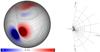 |
Fig. 1. Radial magnetic field distribution on the solar surface with a strong dipole at the equator and four weaker dipoles at higher latitudes in the northern hemisphere (left). The two thick black lines represent the equatorial and parasitic dipole polarity inversion lines. Longitudinal 2D Sections of the grid at Φ = −175° and 5° after the relaxation (right). For more details, see Sect. 2.4. In both panels, the simulation grid is represented with thin black lines. |
The code also uses a flux-corrected transport algorithm (DeVore 1991) that keeps the magnetic field divergence-free with respect to the machine accuracy. It also avoids non-physical results (such as negative mass densities) and minimizes numerical oscillations related to strong gradients that develop at the grid scale.
The numerical domain covers the volume Φ ∈ [ − 180° ,180° ] in longitude, Θ ∈ [ − 84.4° ,84.4° ] in latitude, and R ∈ [1, 33]R⊙, where R⊙ is the Sun’s radius. The domain is periodic in Φ. Along the Θ boundaries, the normal velocity flow and normal magnetic field are reflecting and the tangential components obey a zero-gradient conditions. At the radial inner boundary, we imposed a line-tying condition. At the radial outer boundary, the normal component of the velocity obeys a zero-gradient condition, while tangential components are settled as being zero-valued outside.
2.2. Initial magnetic field
The initial magnetic field is analytically defined, along with its potential. We set a classical Sun-centered dipole with |Br| = 10 G at the poles and at R = R⊙. To build a pseudo-streamer topology, we added two bipolar regions. First, a strong, equatorial dipole deforms the equatorial polarity inversion line between the two solar hemisphere. It stretches the northern coronal hole (region of open magnetic field) to the equator. Second, an extended bipolar region in the north hemisphere separate the equatorial open magnetic field region in two. This extended bipolar region is numerically generated by the combination of three dipoles, whose intensities are given in Table 1. The insertion of a bipolar region in the northern hemisphere generates an ellipsoidal polarity inversion line in addition to the equatorial inversion line and naturally generates a pseudo-streamer topology. In order to reduce the computing time of the relaxation phase that opens the large-scale solar magnetic field under the solar wind kinetic pressure (described in Sect. 2.4), we imposed the magnetic field to be purely radial beyond 2.5 R⊙ by using the potential field source surface model (PFSS; Schatten et al. 1969).
Positions and orientations of the magnetic dipoles as they are used in the ARMS code.
2.3. Pseudo-streamer topology at initial time
The initial magnetic topology of the solar corona, before any relaxation phase, is presented in Fig. 2. The top panel displays particular field lines that exhibit the magnetic topological structures of the modeled corona. Our coronal magnetic model is structured by two particular topological structures: the helmet streamer (HS) and the pseudo-streamer (PS). The helmet streamer is an equatorial structure formed by trans-equatorial closed loops (red and yellow field lines) bordered by open field (blue field lines). The pseudo-streamer topology studied in this paper lies above (since it is generated by) the northern parasitic polarity (Sect. 2.2). It consists of two sets of closed field (green field lines) that form a dome, bordered by both open field (dark blue field lines) and trans-equatorial closed field (yellow and red lines). Using the tri-linear method of Haynes & Parnell (2007) implemented in ARMS by Wyper et al. (2016), we find three magnetic null points in this configuration, denoted as NP1, NP2, and NP3. Two closed separators connect the null points along the apex of the PS closed dome. The two extreme null points (NP1 and NP3) are negative null points and the central one (NP2) is a positive null point. A negative null point is defined as a null point for which the fan magnetic field points toward the null point, and away from the null along the spines, and one eigenvalue is positive while the other two are negatives (or have negative real parts; Priest & Titov 1996; Parnell et al. 1996). Reciprocally, a positive null point has its fan magnetic field pointing away from the null and its spines pointing toward the null, with one negative eigenvalue and the two positives (or have positive real parts). The spines associated to these three null points are represented by violet lines in Fig. 2. In this paper, we use the nomenclature “spines” and “fans,” as defined in Priest & Titov (1996). The fan of a null point is the surface formed by the field lines having the same field direction that originates at the null point, in the plane of the eigenvectors of the matrix of the magnetic gradients at the null point, and whose eigenvalues have the same sign. A spine is the line that emanates from the null point along the remaining third eigenvector. The fans of NP1 and NP3 have dome-like shapes and their spines are radially oriented at the null point. The fan of NP2 is vertical, with partly open field forming a separatrix curtain (Titov et al. 2011) that extends beyond in the heliosphere, and partly closed field belonging to the trans-equatorial closed loops (including, e.g., red loops between NP1 and NP2). The spin of NP2 belongs to the PS closed dome. Although, at this stage, NP3 is bordered by open magnetic field, its fan is not vertical and part of this open field (part at the left of NP3 on Fig. 2 top) belongs to NP2’s fan.
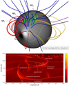 |
Fig. 2. Magnetic configuration of the corona before relaxation. Top: characteristic field lines that highlight the main magnetic topological structures and connectivity domains of the corona (see Sect. 2.4). Blue lines are open field lines, green lines are field lines closed under the pseudo-streamer dome, and red and yellow lines are trans-equatorial closed field lines. The purple lines show the spines from all three null points, which are labeled NP. Bottom: initial distribution of Q, the squashing factor, in logarithmic scale on the solar surface at initial time (see Sect. 2.4). |
This magnetic topology is identical to that of Aslanyan et al. (2021, 2022), and Wyper et al. (2021): two lobes forming a dome-like structure bordered by both open and trans-equatorial closed field, with three null points and a vertical fan emanating from the null point in the middle (NP2). The main difference lies in the dipoles configuration. Their initial magnetic configuration has two distinct bipolar parasitic regions in the northern hemisphere that generate a slightly longer and narrower pseudo-streamer with a larger null point separation.
The bottom panel in Fig. 2 represents the distribution of the squashing factor in logarithmic scale on the solar surface. The squashing factor, Q, is defined in Titov et al. (2002). If we consider two neighboring footpoints belonging to two different field lines, the squashing-factor Q is proportional to how much these field lines diverge from each other. It relates to the gradient of magnetic connectivity. We used the tri-linear method developed by Haynes & Parnell (2007) We computed the squashing factor Q using the method implemented by Wyper et al. (2021) in ARMS. Red regions represent low Q while yellow regions highlight high Q, (i.e, small and large region connectivity gradient respectively; Titov et al. 2002; Titov 2007; Pariat & Démoulin 2012). By definition, QSLs are regions with a squashing factor of Q ≫ 1, while surfaces with theoretically infinite-Q are called separatrices and they divide distinct connectivity domains. The fan surfaces are separatrices. In the bottom panel of Fig. 2, the intersection of the separatrices with the solar surface are embedded in high-Q regions, highlighted in yellow. The PS closed dome photospheric trace forms an ellipsoidal shape and the footpoints of the vertical fan are located along the intense yellow line enclosed in the ellipsoidal structure. We identified distinct connectivity domains. Two open magnetic field domains corresponding to the north and south coronal holes, located northward of the yellow line connecting [Θ, Φ] ≃ [70° , − 90° ] and [Θ, Φ]≃[30° ,90° ] and southward of the yellow line connecting [Θ, Φ]≃[−15° , − 90° ] and [Θ, Φ]≃[−45° ,90° ]. A third open-field region is located in the high-Q triangular shape centered at [Θ, Φ]=[15° , − 15° ]. The open field connectivity domain are shown by the blue field lines in Fig. 2 (top panel). A closed-field region is confined below the PS separatrix dome (green field lines), namely, their footpoints are anchored inside the ellipsoidal high-Q shape between Θ ≃ +10° and Θ ≃ +60°. Finally, trans-equatorial closed magnetic field connect the two solar hemisphere between −60° and +70° (red and yellow field lines).
Initially (t = 0), the northern and the equatorial coronal holes are linked by a narrow corridor, on the western part of the PS closed dome (positive longitudes), between the green and yellow field lines.
2.4. Atmosphere and relaxation phase
We initialized the atmosphere using the 1D Parker solution (Parker 1965) that describes an isothermal solar wind:
 (4)
(4)
where v(r) is the radial velocity,  is the isothermal sound speed, and rS = G M⊙mp/4kBT0 is the radius of the sonic point. We assumed a constant temperature T0 = 1 × 10⁶ K giving a sound speed cS = 129 km s−1 and rS = 5.8 R⊙. The inner-boundary mass density is a free-parameter that we set at ρ(R⊙) = 3.03 × 10⁻¹² kg m−3. This provides an isothermal atmosphere stratified in density with a radial plasma flow.
Because of the wind flow, the system is initially out of a force balance. The system needs to be relaxed to reach a quasi-steady state in which the magnetic forces and the kinetic pressure of the wind compensate for this insufficiency. As detailed in Sect. 2.2, we used a PFSS model to open some of the magnetic field initially. The position of the source surface implies an overestimation of the amount of open magnetic flux. We first ran the simulation without dynamically refining the grid and we let the system relax until the magnetic and kinetic energy became almost constant. The relaxation phase duration is 545τ = 5.45 × 10⁴ s. We note that τ = 100 s is the typical Alfvén time, calculated with vA ≃ 1500 km s−1, which is the typical Alfvén velocity below the two pseudo-streamer lobes of closed field and L ≃ 150 Mm the length between the two footpoints of the longest closed loop below the PS dome.
During this relaxation phase, part of the open field of the disconnected coronal hole closes down, connecting the two solar hemispheres. Figure 3 presents the squashing-factor map in logarithmic scale at the solar surface after the relaxation. In the rest of the paper, we define t = 0, the initial time when the relaxation phase ends. At the end of the relaxation, the size of the northern polar coronal hole and the disconnected coronal hole (see insert in Fig. 3) decreased significantly. Even though the size of the disconnected open field region decreased, our magnetic configuration keep its pseudo-streamer topology. It is worth mentioning that the right part of the disconnected coronal hole is slightly stretched to the west and forms a very narrow open-field corridor between both trans-equatorial and pseudo-streamer closed fields.
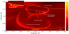 |
Fig. 3. Distribution of log Q after the relaxation. The yellow-colored separatrices delineate the connectivity domains: trans-equatorial streamer loops, pseudo-streamer loops (both closed field), and polar and equatorial coronal holes (open field). The size of the equatorial coronal hole (see inserted panel) is significantly reduced during the relaxation. |
The final pseudo-streamer topology after the relaxation is shown in Fig. 4. While the topological skeleton remains the same, we notice two specific changes in the magnetic configuration. Since some of the initially open field ends up closing, NP3 is no longer located in the open part of the vertical fan; instead, it belongs now to the trans-equatorial closed field located in the west. Therefore, the initially open spine of NP3 closes down during the relaxation and the thin open corridor initially connecting the northern polar CH and the open field south of the parasitic bipolar region disappears. The open field region south of the PS dome is now disconnected from the north polar coronal hole.
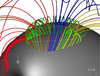 |
Fig. 4. Pseudo-streamer topology at the end of the relaxation phase. The magnetic field at the solar surface is colored in gray scale. The white lines draw the polarity inversion lines. The green loops materialize the PS closed dome separatrix, the dark blue lines show the open section of the vertical fan associated to NP2. The sections of the red and yellow lines above the PS dome (green lines) show the closed section of the vertical fan while the section of the red and yellow lines lying along the green field lines show the closed fan associated with the secondary null points (NP1 and NP3). |
On the squashing-factor map (Fig. 3), we identified four specific points located at the intersection of three high-Q segments. These four points: [Θ, Φ]=[12.4° , − 9.0° ], [Θ, Φ]=[52.1° ,18.5° ]; [Θ, Φ]=[−4.0° ,14.3° ]; and [Θ, Φ]=[49.1° ,28.0° ] are named the triple points. A triple point is the photospheric trace of the joining of two quasi-separatrix layers. It separates three different connectivity domains: a first one enclosed below the pseudo-streamer closed separatrix dome, a second one that is open in the disconnected open field region, and a third closed below the helmet streamer (see Fig. 2). The four triple points appeared with the closure of the open field corridor.
2.5. Photospheric forcing
In order to energize the system, we applied a sub-Alfvénic photospheric flow in the parasitic negative polarity. The photospheric forcing is applied inside the ellipsoidal PIL and forces the closed field confined below the PS dome. We chose to impose a smooth and large-scale rotational photospheric flow to coherently force the pseudo-streamer configuration and mimic the slow shear of the polarity inversion line. The spatial profile of the photospheric flow depends on the gradient of the radial magnetic field, Br, and is defined as:
![Mathematical equation: $$ \begin{aligned} \boldsymbol{v_S}(R_\odot , \Theta , \Phi ) = { v}_0 \sin \left[\pi \left( \frac{B_{\rm r}(R_\odot ,\Theta ,\Phi )-B_{\rm max}}{B_{\rm max}-B_{\rm min}}\right)\right] \left(\boldsymbol{e_r} \times \mathbf \nabla _t B_r (R_\odot ,\Theta ,\Phi )\right), \end{aligned} $$](/articles/aa/full_html/2023/07/aa45611-22/aa45611-22-eq6.gif) (5)
(5)
with v0 as the maximum velocity, Br as the radial component of the magnetic field, and Bmax and Bmin, respectively, as the minimum and maximum values of Br that define the region where the flow is applied. We chose a maximum velocity of 115 km s−1, which corresponds to a velocity of 7.67% of the mean Alfvén speed in the parasitic polarity. While it is faster than the observed photospheric flows at the solar surface, it remains consistent with sub-Alfvénic photospheric motions.
We chose Bmax = −4 G and Bmin = −16 G so that the elliptic profile is sufficiently thick to shear enough magnetic flux closed below the PS dome and that the flow is close to the PIL but zero-valued at the PIL itself (see Fig. 5). As described in Masson et al. (2019), such a spatial profile does not modify the radial component of the magnetic field. It only slightly perturbs the magnetic topology without making the pseudo-streamer structure disappear.
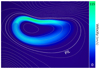 |
Fig. 5. Photospheric boundary forcing motion with a circular velocity flow. The white lines represent iso-contours of the radial magnetic field. The thick white line is the polarity inversion line. |
The velocity flow is gradually applied by adding a temporal ramp using the cosine function below:
![Mathematical equation: $$ \begin{aligned} a(t)=0.5 \left[1-\cos \left(2 \pi \frac{t-t_{\rm min}}{t_{\rm max}-t_{\rm min}}\right) \right], \end{aligned} $$](/articles/aa/full_html/2023/07/aa45611-22/aa45611-22-eq7.gif) (6)
(6)
with tmin = 0 and tmax = 45, respectively, as the initial and final time of application of the flow. The velocity profile reaches its maximum value at t = 22.5 τ = 2250 s.
3. Dynamics of the pseudo-streamer
In this section, we present the dynamics of the pseudo-streamer magnetic field. We first show the formation and global evolution of the electric currents in the pseudo-streamer topology (Sect. 3.1). We then highlight the impact of pseudo-streamer reconnection away from the Sun (Sect. 3.2). Then, we define the used method for the connectivity analysis (Sect. 3.3). Finally, we describe the dynamics of the pseudo-streamer magnetic field accordingly with respect to the associated topological elements (Sects. 3.4–3.6).
3.1. Formation and evolution of current sheets
The photospheric forcing applied inside the parasitic polarity (see Sect. 2.5) shears the magnetic flux closed below the separatrix dome. Figure 6 displays a 2D cut in the (r, Θ) plane at Φ = −5° of the electric current density that forms along the sheared magnetic loops and corresponds to the most intense arc lying just above the north section of the ellipsoidal polarity inversion line (PIL) at t = 16.5 τ and t = 29.5 τ.
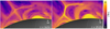 |
Fig. 6. Current density distribution on longitudinal Section, at times t = 16.5 and t = 29.5τ for longitude Φ = −5°. The white letter N and the associated arrow indicate the north direction. |
As a consequence of the photospheric flow, the forced closed loops inflate and push the overlying closed field toward the separatrix dome. This compression leads to the formation of electric current sheet along the separatrix surface (Galsgaard et al. 2000). In Fig. 6 (left panel), the 2D cut of the current density highlights the 2D geometry of the separatrix dome, with the two well defined lobes shown just as in a standard null-point topology (Masson et al. 2012). Initially, the angle at the intersection between the dome separatrix and the vertical fan is close to 90°, forming a X-point type current structure localized at the closed separator. As the system is forced, the growth of the sheared closed-loops compresses the separatrices (dome and vertical fan) leading to the shear of the separator current sheet as shown in Fig. 6, right panel (Parnell & Haynes 2010; Pontin et al. 2013). This deformation and the associated increase of electric current density strongly suggest that magnetic reconnection can develop between the magnetic flux below the northern lobe of the pseudo-streamer and the magnetic field located southward of the southern lobe.
3.2. Impact of pseudo-streamer reconnection at 5 R⊙
The photospheric forcing of the pseudo-streamer and the build-up of electric currents at the pseudo-streamer interface (cf. previous section) lead to substantial amount of interchange reconnection. In order to visualize the impact of such magnetic reconnections in the inner-heliosphere, Fig. 7 presents the location at 5 R⊙ which have been magnetically connected to a reconnecting field line during the course of the simulation. At this altitude, the magnetic field is open everywhere. The points displayed in this map can either be magnetically connected to the polar coronal holes or the equatorial coronal hole. Figure 7 outlines the heliospheric S-web (Higginson et al. 2017a) associated with the pseudo-streamer configuration. The black area delimits the connectivity region associated with the three different coronal holes. In particular, the central domain corresponds to the disconnected equatorial coronal hole. Such structure is classically observed in model of pseudo-streamers (Titov et al. 2011; Scott et al. 2018; Aslanyan et al. 2022). Even though the equatorial coronal hole has a limited extend on the solar surface, on the order of 2° in latitude and 4° in longitude at the beginning of the relaxation (see Fig. 3), its imprint in the inner heliosphere is far larger, spanning over a domain that extend over 15° in latitude and 20° in longitude at 5 R⊙. The connectivity domain of the disconnected equatorial coronal hole has a solid angle that is about one order of magnitude larger at 5 R⊙ than on the solar surface.
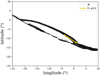 |
Fig. 7. Longitudinal-latitudinal connectivity map at 5 R⊙ displaying locations impacted by reconnection at the pseudo-streamer. The magnetic field lines connected to the black point in the figures have experienced at least one episode of magnetic reconnection during the course of the simulation. The yellow line traces the path of the intersection with the 5 R⊙ sphere of the magnetic field line n° 20, as it slip-reconnects (see Sect. 3.7). |
Black areas are locations where the passing magnetic field lines have had at least one episode of interchange reconnection, namely, they have, at one moment in time, reconnected with a closed coronal loop; hence, their footpoint at the solar surface has experienced a drastic change of position, going from one coronal hole to another. To plot this map, we generated 22 400 magnetic field lines homogeneously distributed across the S-web arcs region at R = 5 R⊙ and recorded their positions at the surface for each time step. Over the computation time, if a shift in the latitude of the photospheric footpoint is greater than 20° between two consecutive output time steps (25 s), we associate it with the interchange reconnection. The choice of 20° derives from the latitudinal extend of the pseudo-streamer. In the case of our pseudo-streamer, the equatorial coronal hole is separated by a latitudinal angle of the order of 30° (see Fig. 4). Interchange reconnection at the pseudo-streamer thus induces a change of at least 30° in latitude of the photospheric footpoint. We checked that changing the threshold angle in the interval [1° ,25° ] does not qualitatively change the resulting connectivity map.
While studying the impact of interchange reconnection at pseudo-streamer on the heliosphere, it is fundamental to understand the generation of the slow solar wind (e.g. Higginson et al. 2017b; Wyper et al. 2022), it is necessary to first carefully explore the topological evolution in the presence of a pseudo-streamer, which is the objective of this study.
3.3. Analysis method and global dynamics
In order to determine the dynamics of the magnetic field connectivity, we selected specific field lines and plotted them from fixed footpoints at the solar surface. Those field lines with fixed footpoints have been selected outside of any photospheric flows (Sect. 3.1). In addition, the line-tying condition at the inner boundary ensures that following the evolution of the conjugate footpoint for each selected field line allows us to determine the connectivity dynamics of our pseudo-streamer topology.
The time between two simulation outputs is 25 s = τ/4 (see Sect. 2.5). We limit the analysis to the time interval t ∈ [0, 29.25] τ. Indeed, after t = 29.25 τ, the photospheric flow starts to deform the inner part of the vertical fan. The sheared closed field starts to be more twisted than sheared as in Wyper et al. (2021), and the vertical fan photospheric trace, anchored in the parasitic polarity, displays a Z-shape at its two extremities located at [Θ, Φ]=[37.4° , − 26.5° ] and [Θ, Φ]=[18.8° ,25.2° ]. The aim of this study is to accurately determine the dynamics of the magnetic field during a gradual evolution of a pseudo-streamer as observed in the corona (Masson et al. 2014). Thus, by limiting our analysis in time we avoid including any specific dynamics due to an unrealistic forcing as it develops with time in our simulation.
In order to identify all reconnection episodes developing during the pseudo-streamer evolution, we selected 20 regions distributed along the separatrix dome in the inner and outer connectivity domains. All 20 regions are shown in Fig. 8. In each of those 20 regions, we selected a point on the separatrix at the solar surface and we plotted a group of ten field lines from fixed footpoints along a straight segment orthogonal to the photospheric trace of the separatrix dome. The distance between two neighboring footpoints is 0.001°, namely, 1.2 × 10⁻² Mm, in latitude or longitude, depending on the region. We defined a color code for the selected field line to describe the connectivity evolution. A color is associated with a specific connectivity evolution. The color code is described in the Fig. 8 caption. In the following sections, we selected particular field lines displaying a behavior typical of each of the 20 regions. For each fixed footpoint, we plot the magnetic field line and study its dynamics by following the conjugate footpoint connectivity with time. Figure 9 displays the global evolution of the magnetic field connectivity for each selected field line. The color code for the field lines is the same in Fig. 9 as it is in Figs. 8 and 10–12. For clarity, we also give a number to each field line that we use together with the color code.
 |
Fig. 8. Cartoon of the connectivity map at t = 0 summarizing the connectivity evolution of particular magnetic field lines during the forcing stage. The colors of the map behind the points represent all three connectivity domains at t = 0: green for magnetic field closed below the PS dome (P), blue for open field (O), and red for trans-equatorial closed field (T). The size of the equatorial coronal hole is voluntary magnified, for readability reasons. The fixed footpoints of the selected field lines are represented by circles whose color are the same as used in Fig. 9 and Figs. 10–12. The colors correspond to particular connectivity evolution detailed in Sects. 3.4–3.6, depending on the connectivity states that a given field line has among P, T, and O states. For example T → P means the field line was a trans-equatorial loop before the reconnection and a pseudo-streamer loop after the reconnection. |
From the global dynamics, we identified three types of sequential episode of magnetic reconnection depending on the location and the connectivity domain involved. For simplicity in the notation, we associate a letter to each of the three connectivity domains. The closed connectivity domain below the PS dome is denoted P for pseudo-streamer closed field, the connectivity domain closed below the streamer but outside of the PS dome is denoted T for trans-equatorial closed field, and O is for the open field domain either in the polar coronal hole (CH) or in the island of the open field at low latitude (see Fig. 8). In Fig. 9 and the associated animation, we observe several episodes of connectivity changes, highlighting that magnetic reconnection is occurring. Thus, we identified a closed-closed reconnection episode between the P and T closed field, and an interchange reconnection between either the P closed field or the T closed field and the open field O. In the next three sections, we present in detail those reconnection episodes.
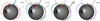 |
Fig. 9. Global evolution of the field lines connectivity in a pseudo-streamer topology. The color code is the same as in Fig. 9: it associates a color to a particular connectivity evolution. It is the same code as in Figs. 10–12. It is described in Sects. 3.4–3.6. The field lines presented here are characteristic of the nearby regions. An animation of this figure is available online. |
3.4. Closed-closed reconnection
We first analyze the connectivity evolution of the initially P closed loops and T closed loops far from the open field region, that is, on the east and west sides of the pseudo-streamer topology, corresponding to lines n° 1 to 11. Depending on the location and the initial connectivity of the field lines, we identified different types of magnetic reconnection episodes involving a closed magnetic field.
Figure 10 shows the field lines that change their connectivity only through closed-closed magnetic reconnection. The two magnetic fluxes that reconnect together and exchange their connectivity correspond to the magnetic flux anchored on each side of the elliposidal PIL (region colored in red on Fig. 8). For each northern and southern flux, we have two connectivity domains: the P closed loops enclosed below the PS closed dome separatrix and the T closed loops with trans-equatorial connections. In the following, we only use the connectivity types of P-type and T-type closed loops. We do not distinguish the magnetic field lines anchored south and north of the parasitic polarity.
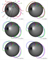 |
Fig. 10. Connectivity evolution of pseudo-streamer field lines in the closed-connectivity domain on the sides of the pseudo-streamer topology. The dynamics is a pure closed-closed dynamics between trans-equatorial loops and pseudo-streamer loops. An animation of this figure is available online. |
Red field lines (see Fig. 10, field lines n° 3, 7, and 8) are initially trans-equatorial loops. They reconnect with the P closed field only once in the simulation and thus exchange their connectivity, namely, the reconnection episode is T → P connectivity evolution. Blue field lines (n° 1, 2 and 5) display the opposite change of connectivity: P closed-loops reconnect with T closed loops which corresponds to P → T dynamics (see Fig. 8). Green and fuchsia field lines present two successive reconnection episodes. Green field lines (n° 4, 6, 9 and 11) are initially P closed loops. They first reconnect with the T closed loops and then reconnect back with P closed loops. This succession of magnetic reconnection episodes correspond to the P → T →P dynamics (see Fig. 8). The fuchsia field line n° 10 has the opposite evolution, corresponding to T → P → T dynamics.
This closed-closed reconnection mainly occurs at the east and west side of the pseudo-streamer topology, where only the two closed type (P and T) of connectivity domain are in contact along the PS separatrix dome. In each of those two specific regions, a null point with a closed outer spine line is present, with NP1 and NP3 on the east and the west, respectively. Moreover, a closed separator connects those two null points and the third one (NP2). Thus, the closed-closed reconnection can occur either at NP1, NP3 (Galsgaard et al. 2000) or at specific locations along the closed separator where the parallel electric field is strong enough (see Parnell & Haynes 2010).
3.5. Opening of the P closed field by a single episode of interchange reconnection
A second type of connectivity evolution is the opening of initially closed field (Sect. 2.2) through interchange reconnection. Such reconnection defines magnetic reconnection between an open and a closed field. In a pseudo-streamer topology, the closed field that reconnects with the open one can be initially closed below the PS dome (P) or closed below the streamer (T). The magnetic field involved should be near the section of the PS separatrix dome interfacing the open field (O) and the pseudo-streamer closed field (P). An interchange reconnection between the T closed loops and the open field is expected to occur along the open separator created by the intersection of the vertical fan and the streamer open-closed separatrix surface on each side of the pseudo-streamer.
For a given field line, the surrounding magnetic field in a region within a radius of 0.02° = 0.5 Mm has the same connectivity state and presents a similar connectivity evolution. This region of identical connectivity evolution is large compared to the distance between two adjacent plotted field line footpoints that is 0.001° = 2.5 × 10⁻² Mm and the highest grid resolution, which is 10−6 ° resolution (25 m) in the parasitic region.
Figure 11 illustrates the four different connectivity evolution for each of the four different regions, characterized by four field lines numbered from 12 to 16. The violet field line (n° 13) is initially open southward of the elliptic PIL and reconnects once during the simulation, by closing directly under the pseudo-streamer dome at t ∼ 16.25τ (O → P evolution). Bordering the northern coronal hole, the cyan open field line n°16 has two episodes of reconnection. It first closes under the PS dome between t ∼ 17 τ and 21 τ and then opens after t = 21.25 τ. It defines the O → P → O evolution (Fig. 8). The orange field lines (n°12 and 15) present the opposite evolution of connectivity, P → O → P. They start as initially P closed loops, then they open at early stage between t ∼ 2 τ and t ∼ 6 τ, and they close again later in the simulation between t ∼ 12 τ and t ∼ 16.75 τ.
 |
Fig. 11. Evolution of the field lines connectivity nearby the section of the PS dome separatrix surface delimiting open and PS closed fields. The north direction is indicated by the arrow and the letter N at the bottom left of the first figure. An animation of this figure is available online. |
The field lines n° 12, 13, 15, and 16 do not transition through a trans-equatorial loop before opening. We note that the olive field line n° 14 has a different dynamics that will be described in the Sect. 3.6. Our results show that interchange reconnection leads to the exchange of connectivity between open and closed magnetic field at the coronal hole boundary and at the isolated open field region disconnected from the CH by the parasitic polarity. This interchange reconnection is localised along the section of the PS dome separators connected to the central null point (NP2).
3.6. Successive episodes of magnetic reconnection
3.6.1. Multi-reconnection episodes in the open field thin corridor
While located inside the isolated open field region, the olive line (n°14, see Fig. 8) does not simply close below the PS dome through a single interchange reconnection episode but it closes through two successive reconnection episodes. First, it becomes a T closed loop at t = 5 τ. There are two explanations: there is either an interchange reconnection along the helmet streamer open-closed separatrix surface or a closure with another open field line at the apex of the helmet streamer as a consequence of the wind (see Sect. 2.4). Second, it reconnects with a P closed loop at t = 17 τ and closes below the PS dome. It thus goes through all three connectivity domains, successively.
As shown in the insert panel of Fig. 3 and schematically recalled in Fig. 8, the open magnetic domain south of the PS dome is locally stretched forming a thin open-field corridor elongated over few degrees of longitude. This thin open-field corridor is located between the trans-equatorial (south) and pseudo-streamer (north) closed field regions. The separatrix surfaces delimiting the P closed and open regions on one hand and the T closed and open regions on the other hand, are very close to each other. Thus, the proximity of these separatrix surfaces favors magnetic reconnection at either separatrix surface for the field anchored nearby.
3.6.2. Multi-reconnection episodes at the triple points
As described in Sect. 2.2, in our pseudo-streamer configuration, there are four triple points (see Sect. 2.2 for their definition) localized at the intersection of the P closed field, the T closed field and the open field from the isolated open field region and the coronal hole. Thus, it is in theory possible to have successive reconnection episodes combining closed-closed reconnection and interchange reconnection for the magnetic flux anchored in the vicinity of those four triple points.
In Fig. 12, we plotted field lines with fixed footpoints close to the triple points to determine the dynamics of magnetic reconnection. The brown line n° 17 and yellow line n° 20 reconnect several times and jump in the three connectivity domains intersecting at the triple point, successively. The brown field line n°17 has a P → O → T → P evolution: initially closed under the dome, it first opens by interchange reconnection at t = 13.50 τ then closes trans-equatorially at t = 13.75 τ and eventually reconnect back into a pseudo-streamer loop below the dome by a closed-closed reconnection at t = 14.00 τ. The yellow line n° 20 is also initially closed below the PS dome. At t = 12.75 τ it reconnects with the trans-equatorial field and becomes a T closed loop and at t = 13.50 τ the field opens through interchange reconnection. The khaki field line n° 19 has a O → T → O → P at early time: initially open, it first closes across the equator at t = 2.75 τ, then opens at t = 3 τ, and eventually closes below the PS dome at t = 6.5 τ.
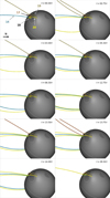 |
Fig. 12. Connectivity evolution of the four triple points, that are points where the three connectivity domains are in contact. In particular, the black and white field lines (n°18) are separated by 2.5 × 10⁻² Mm and highlight two particular dynamics. The north direction is indicated by the arrow and the letter N at the center right of the first figure. An animation of this figure is available online. |
Field lines n°18 regroup four field lines under the same number for readability but with different colors (yellow, black, grey, and white). They are only separated by a distance of 25 × 10−2 Mm. The yellow field line n° 18 has a P → T → O → T → P evolution scenario: first, it undergoes a closed-closed reconnection at the closed separator current sheet and becomes a T closed loop at t = 2.25 τ, then it opens by interchange reconnection at t = 5.50 τ and closes again below the helmet streamer (HS) at t = 6.00 τ. It finally reconnects one last time to close down below the PS dome t = 28.50 τ. The black, white, and grey field lines, undergo much more episodes of magnetic reconnection. An animation is available online, associated with Fig. 12. The white and grey lines have several back and forth reconnections during the simulations between the two closed field connectivity domains P and T. This back and forth reconnection is observed around five times for those two field lines (P → T or T → P). This dynamics is also observed for the black line, but to a much lesser extent. After the multiple closed-closed reconnections, the black, grey, and white field lines both open through interchange reconnection either from a T closed loop or a P closed loop state. Some back and forth reconnections were also noticed between the open and the closed connectivity states (e.g., for the white line P → O → P → T → O → P).
Because of the proximity of all three connectivity domains at the triple points, footpoints of two field lines separated by a small distance may present significant dissimilar behaviors. That is the case for the black, white, and grey field lines (lines n° 18). Even though they undergo multiple reconnection episodes between all three connectivity domains, the sequence of reconnection episodes is not the same for each of the three field lines. This dynamics create a more complex and exotic scenario based on multiple episodes of reconnection that open the magnetic field initially closed below the PS dome. Every field line (n° 18 to 21) go through all three connectivity domains, which highlight the coupling between pseudo-streamer and helmet streamer through magnetic reconnection. The back-and-forth behavior of field lines n° 18 is clearly more important than the other field lines anchored closed to the three other triple points. According to the dynamics of the field line n° 14 (see Sect. 3.6.1) located in the thin corridor of open field associated with the triple point close to the field lines n° 18, we suggest that the multiple back-and forth reconnection is a direct consequence of the combination of the thin elongated shape of the open field region and the presence of a triple point.
3.7. Slipping reconnection
Finally, we explored the behavior of the newly opened magnetic field. Figure 13 presents the field line evolution for two particular field lines studied in Sects. 3.5 and 3.6: n°16 (cyan) and n°20 (yellow). After opening, these field lines show an apparent slipping motion, moving toward lower longitudes. During this process, they remain open and do not undergo multiple interchange or closed-closed reconnection, unlike the field lines close to the triple point (see Sect. 3.6).
 |
Fig. 13. Temporal evolution of the field lines n° 16 (cyan) and 20 (yellow). An animation of this picture is available online showing such apparent slipping motion for both lines. |
To quantify those field lines displacement and their associated velocity we extracted their positions at a radial distance of R = 2 R⊙. At each time step, we extract the (Θ, Φ) position of all the points along the considered field line obtained from our tracing routine. In order to obtain the exact position of the line at 2 R⊙, we perform a linear interpolation at 2 R⊙ of the coordinate position (Θ, Φ) of the field line. Figure 14 top panel displays the time evolution of the longitude (Φ) and latitude (Θ) of the intersection of the 2 R⊙ sphere and the field lines n°16 (cyan) and n°20 (yellow). In both case, we observe a displacement of ΔΦ ∼ 2 − 3° in Φ and ΔΘ ∼ 1 − 2° in Θ, which corresponds to a global displacement of 29.9 Mm for the cyan field line and 40.3 Mm for the yellow field line. Both field lines move toward positive latitudes and negative longitudes. After t = 25 τ (the black, dashed line in Fig. 14), the displacement of field line n°16 (cyan) becomes smaller and it displays some oscillation along Φ.
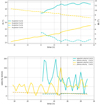 |
Fig. 14. Evolution of the Θ (latitude, solid line) and Φ (longitude, dashed line) components of the field lines n° 16 (cyan) and 20 (yellow) at 2 R⊙ (top). Tangential velocity of the field lines n° 16 (cyan) and 20 (yellow) calculated at 2 R⊙ between t = 17.75 τ and t = 29.25 τ (bottom). The cyan and yellow dashed lines display the tangential plasma velocities at 2 R⊙ at the location of the footpoints of the associated field lines. The vertical dashed back line indicates the end of the large, rather straight slipping motion for the cyan field line (n° 16) and the beginning of the oscillations. |
Such apparent slipping motion of open field lines suggests that slipping reconnection can be responsible for the dynamics of those field lines. If slipping reconnection is involved, the apparent velocity of the field lines should be higher than the local plasma velocity (Masson et al. 2012; Janvier et al. 2013). Thus, we computed the tangential velocity at 2 R⊙ of the yellow and cyan field lines and compared it with the plasma tangential velocity at the location of the field-line footpoints at the 2 R⊙ sphere. Figure 14, bottom panel, shows the tangential velocity for the selected field lines and the plasma. While the plasma velocity (colored dashed lines in Fig. 14 bottom panel) ranges from 0 to 20 km s−1, the field line velocities (colored solid lines in Fig. 14 bottom panel) ranges between 40 km s−1 and 200 km s−1, which is much higher than the plasma speed. The oscillations in the field line velocity show that the evolution is impulsive, while the plasma velocity remains stable throughout the simulation.
According to our velocity analysis, the apparent motion of field lines results from slipping reconnection and not from the advection of the field by plasma motions. Slipping reconnection consists of exchanging the connectivity between two neighboring field lines belonging to a quasi-separatrix layers (Aulanier et al. 2006; Masson et al. 2012; Janvier et al. 2013). In our simulation, the slipping open field lines belong to the quasi-separatrix layer embedding the pseudo-streamer vertical fan. Thus, in addition to the multiple reconnection episodes, once the field lines open, they can keep reconnecting across the QSL vertical fan in the open section of the vertical fan.
In order to have an insight into these slipping motions in the heliosphere, the path of the apparent motion of field line n° 20 at R = 5 R⊙ is traced in Fig. 7. The path of the motion of field line n° 16 is not represented since it is basically the same as the field line n° 20, for longitudes Φ ∈ [ − 5° ,0° ], but occurring at different time steps. The magnetic field lines slip over several degrees along the arc of open-closed connectivity changes described in Sect. 3.2.
4. Conclusion and discussion
In this paper, we provide a self-consistent model of the pseudo-streamer dynamics and study the connectivity evolution of a pseudo-streamer magnetic field. We modeled the solar corona, up to 30 R⊙, in a quasi-steady state, having an equatorial coronal hole disconnected from the polar coronal hole associated with a pseudo-streamer topology (see Sects. 2.3 and 2.4). The pseudo-streamer (PS) is associated with three null points, which is one of the simplest topology for a pseudo-streamer (Titov et al. 2011; Scott et al. 2019, 2021). Our magnetic configuration is consistent with pseudo-streamer configuration reconstructed from observed magnetograms (Masson et al. 2014; Titov et al. 2012). We forced the system by applying a large-scale slow photospheric velocity flow below the PS dome, without forcing the open-closed separatrix surfaces directly. We performed a fine analysis of the magnetic field dynamics. To do so, we selected field lines belonging to the pseudo-streamer configuration and plotted from a fixed footpoints at the photosphere and analyzed the connectivity of their conjugated footpoints. We identified several connectivity histories depending on the location of the magnetic field lines in the pseudo-streamer topology.
As described in Sect. 3.5, the pseudo-streamer field lines in the closed-connectivity domain on the sides of the pseudo-streamer topology change their connectivity only through closed-closed magnetic reconnection. During their evolution the field lines are closed either below the PS dome or in the trans-equatorial (helmet-streamer) loops. The opening of the pseudo-streamer field occurs by interchange reconnection in the closed-separators current sheet between the field enclosed below the PS dome and the open field from the coronal hole and the isolated open field region. This confirms that magnetic field in a pseudo-streamer can open following the standard one-step interchange reconnection (Aslanyan et al. 2021, 2022). However, we also discovered that this one-step interchange reconnection is not the only way to open or close the pseudo-streamer magnetic field and we identified more complex scenarios where successive reconnection episodes occur. Our results highlight that the pseudo-streamer closed field anchored in the vicinity of triple points goes through at least two reconnection episodes. First, it reconnects with the trans-equatorial closed loops and opens later at the open separator associated with the open-closed streamer separatrix surface (Sect. 3.6). This confirms the scenario proposed by Masson et al. (2014). Those reconnection episodes occur successively and several times producing a back-and-forth dynamics of the field lines anchored in the vicinity of the triple points. Moreover, the magnetic field initially open and anchored in the thin corridor of open field also experiences several reconnection episodes. First, it closes down below the helmet streamer (HS) by interchange reconnection at the open separator and reconnects a second time to close down below the PS dome (Sect. 3.6). Such dynamics indicate that the field can easily experienced several reconnection episodes when it is anchored in a narrow corridor of open field. It is worth mentioning that the field lines are going through more back-and-forth reconnection when they are anchored close to the triple point and in the thin open corridor. This suggest that the combination of the two may be a factor that increases the variability of the opening and closing of the field in a pseudo-streamer topology. Finally, the newly open field lines have an apparent slipping motions. By comparing the plasma velocities and the apparent velocity of those open field lines at R = 2 R⊙, we show that these apparent slipping motions are the signature of slipping reconnection (Aulanier et al. 2006; Masson et al. 2012; Janvier et al. 2013).
We performed a series of numerical studies to understand the open-closed dynamics in pseudo-streamer topology. By applying photospheric flows that emulate super-granular motion at the open-closed boundaries in a similar magnetic configuration than ours, Aslanyan et al. (2021) showed that open and closed field exchange their connectivity by interchange reconnection. Their analysis was designed to determine the connectivity state, open or closed, of each photospheric point near the open-closed separatrix surface. Therefore, they did not unambiguously conclude on the intrinsic dynamics of reconnected field lines. In our study, we applied our photospheric flow far from the separatrix surface footpoints. It allowed us to obtain the generic dynamics of the pseudo-streamer field without drastically modifying the open-closed boundaries. As suggested by Aslanyan et al. (2021), we showed that 1) interchange reconnection occurs at the PS closed separators current sheet and at the open-closed separatrix of the streamer; and 2) the field goes through several episodes of reconnection leading to a back-and forth evolution between the three connectivity domains.
By extending their analysis, Aslanyan et al. (2022) showed that interchange reconnection is more efficient at the PS dome separatrix than at the helmet-streamer open-closed boundary. In this paper, we improve on this result by highlighting that the dynamics of the field is more complex than an open-closed transition. We provide the whole dynamics of the reconnected magnetic field complex evolution depending on the location of the field with respect to the pseudo-streamer topological elements. Moreover, our results also confirm the coupling between the pseudo-streamer and the helmet-streamer closed field through closed-closed reconnection as first suggested by Masson et al. (2014). Such a coupling between pseudo-streamer and helmet-streamer field has been also found in numerical studies of flux-rope eruption (Wyper et al. 2021). This coupling is most likely to also be present in Aslanyan et al. (2021, 2022), but those studies considered only a single type of closed field and did not distinguish between the pseudo-streamer and the helmet-streamer closed field.
Our study has several implications on the processes of injection of plasma into the interplanetary medium, namely, on the generation of the slow wind. Our findings are as follows.
-
While studying individual field lines to understand the details of the pseudo-streamer dynamics, we also determined the heliospheric distribution of the magnetic flux which opened by one or more reconnection episodes (Sect. 3.6). The newly open flux extends over the whole heliospheric arc associated with the vertical fan and its surrounding QSL (Sect. 3.7). By opening the magnetic field all over the pseudo-streamer arc, our model strongly supports the S-web model (Antiochos et al. 2011; Linker et al. 2011) as a major contributor of the slow wind generation through interchange reconnection in pseudo-streamer topology.
-
Our model naturally leads to a diversity of plasma properties in the slow solar wind. The complex nature of the topology of the pseudo-streamer leads to different scenarios of opening of magnetic field lines (cf. Sects. 3.5 and 3.6). In each scenario, the newly formed open field lines result from reconnection between different connectivity domains with different plasma composition. Thus, our model should not generate an unique uniform plasma flow. However, it may inject plasma coming from different coronal regions with different compositions. It may thus explain some of the observed variability of the slow solar wind (von Steiger & Zurbuchen 2011; Burlaga & Lazarus 2000).
-
The back-and-forth reconnections of field lines close to the triple point or to the narrow corridor of open field (Sect. 3.6.1) may provide an explanation for the variability of the slow wind flows. Indeed, the back-and-forth reconnections identified in our model open and close the magnetic field and thus potentially release sequentially plasma flows into the heliosphere. This back-and forth reconnection does not require a specific photospheric flow, but it is derived from the intrinsic nature of the magnetic skeleton of the pseudo-streamer topology. An alternative and/or complementary mechanism that explains its variability, which also relies on interchange reconnection in a pseudo-streamer topology, is the formation of secondary flux ropes leading to a bursty-type reconnection. Both flux rope formation (Wyper et al. 2022) and bursty-type reconnection (Savage et al. 2012) are strong candidates for explaining some of the variability properties of the slow wind. Another well-documented viable explanation for the slow wind variability is the streamer blob model (Higginson & Lynch 2018; Réville et al. 2020, 2022): magnetic flux ropes are created at the apex of the helmet streamer and released in the heliospheric current sheet. However, streamer plasma blobs seem to be more adapted to explain the periodic density structures identified by Viall & Vourlidas (2015), which show a periodicity of 60 to 100 min.
-
The apparent slipping motions of the newly opened field lines, induced by slipping reconnection (cf. Sect. 3.7), implies that the plasma in these reconnected field lines can be injected over a wide volume of the QSL surrounding the vertical fan and extending in the heliosphere (Sect. 3.2). Thus, contrary to a standard interchange reconnection that only can inject the plasma over a small solid angle corresponding to the size of the newly reconnected flux tube, the slipping reconnection allows for the injection of plasma over a broad range of longitudes and latitudes in the heliosphere, as first described in Masson et al. (2012, 2019) for the escape of energetic particles. The apparent slipping motion of the field lines leads to formation of an extended corridor at high altitude in which slow solar wind plasma is injected. Hence, even the scenarios involving a limited domain at the solar surface (e.g. the triple point) can lead to the generation of a solar wind over a relatively extended volume. We emphasize the importance of taking the slipping motion in the corona into account for correctly tracking the route of the plasma from injection to its propagation heliosphere and coupling the corona and the heliosphere. Moreover, this slipping reconnection process occurs along the high-Q arcs forming the structure of the S-Web model (Antiochos et al. 2011). The injection of plasma over a broad area defined by the QSL arcs provides an additional argument that supports the S-Web model as the coronal source of the slow solar wind.
Our study is in agreement with several observational studies of the generation of the slow wind. First, it agrees with the existing models of slow solar wind based on the opening of magnetic field initially closed below the pseudo-streamer dome: the one-step interchange reconnection was introduced by Titov et al. (2011) and the two-step scenario by Masson et al. (2014). Recently, Chitta et al. (2023) identified outflows in the corona associated with the S-web coronal structures, bringing the first clear evidence of plasma flow injections from pseudo-streamer and streamer topologies. As with such models, the slow wind is localized in the vicinity of the open vertical fan and its surrounding QSL. Second, our model of slow wind generation by the different scenarios of connectivity change, based on interchange reconnection, may not be in contradiction with the expansion factor model (Wang & Sheeley 1990). As argued in Crooker et al. (2012), the slow wind is generated at the boundary between open and closed magnetic field. In these regions, the divergence of the magnetic field is the most important: the open magnetic field has the shape of the pseudo-streamer and helmet streamer structures (cf. Figs. 2 and 4). Finally, as explained in the previous paragraph, this work proposes interesting clues for explaining the variability of the slow wind. Further studies of the plasma dynamics and plasma flows injected in the interplanetary medium based on our model may explain the in situ measurements with Parker Solar Probe (Fox et al. 2016) and Solar Orbiter (Müller et al. 2020). Our model suggests that we expect a variety of plasma outflows depending on the reconnection history of the opening field. Those plasma flows may be observed and characterized using the SPICE instrument (Spice & Anderson 2020) on board Solar Orbiter which can provide composition diagnostics of the coronal plasma outflows. Combined with data from the Solar Wind Analyzer (Owen et al. 2020), those outflows can be linked to the in situ composition measurement of the solar wind. Finally, the Extreme Ultraviolet Imager (Rochus et al. 2020) and Metis coronograph (Romoli et al. 2021) on board Solar Orbiter provide EUV images of the low corona and white light images of the high corona, respectively. With both instruments, the plasma outflows in the corona can be identified, in a similar way as is presented in Chitta et al. (2023).
Movies
Movie 1 associated with Fig. 9 (slipping-motion) Access Supplementary Material
Movie 2 associated with Fig. 10 (global-dynamics) Access Supplementary Material
Movie 3 associated with Fig. 11 (PT-dynamics) Access Supplementary Material
Movie 4 associated with Fig. 12 (OF-dynamics) Access Supplementary Material
Movie 5 associated with Fig. 13 (CC-dynamics) Access Supplementary Material
Acknowledgments
T.P.F., S.M., and E.P. acknowledge the support of the APR program of CNES, focused on the Solar Orbiter mission. This work was also supported by the Programme National PNST of CNRS/INSU co-funded by CNES and CEA, and was granted access to the HPC resources of CINES under the allocations 2020 [A007046331] and 2021 [A009046331] made by GENCI. We thank the Alliance Hubert Curien Program funded by the Ministère de l’Europe et des Affaires Étrangères and the Ministère de l’Enseignement Supérieur et de la Recherche and managed by Campus France. P.F.W. was supported by STFC (UK) consortium grant ST/W00108X/1. C.R.D. was supported by NASA H-ISFM and H-SR research grants.
References
- Abbo, L., Ofman, L., Antiochos, S. K., et al. 2016, Space Sci. Rev., 201, 55 [NASA ADS] [CrossRef] [Google Scholar]
- Antiochos, S. K., Mikić, Z., Titov, V. S., Lionello, R., & Linker, J. A. 2011, ApJ, 731, 112 [Google Scholar]
- Aslanyan, V., Pontin, D. I., Wyper, P. F., et al. 2021, ApJ, 909, 10 [NASA ADS] [CrossRef] [Google Scholar]
- Aslanyan, V., Pontin, D. I., Higginson, A. K., et al. 2022, ApJ, 929, 185 [NASA ADS] [CrossRef] [Google Scholar]
- Aulanier, G., Pariat, E., Démoulin, P., & DeVore, C. R. 2006, Sol. Phys., 238, 347 [NASA ADS] [CrossRef] [Google Scholar]
- Burlaga, L. F., & Lazarus, A. J. 2000, J. Geophys. Res., 105, 2357 [NASA ADS] [CrossRef] [Google Scholar]
- Chitta, L. P., Seaton, D. B., Downs, C., DeForest, C. E., & Higginson, A. K. 2023, Nat. Astron., 7, 133 [NASA ADS] [Google Scholar]
- Crooker, N. U., Antiochos, S. K., Zhao, X., & Neugebauer, M. 2012, J. Geophys. Res., 117, A04104 [NASA ADS] [Google Scholar]
- Del Zanna, G., Aulanier, G., Klein, K. L., & Török, T. 2011, A&A, 526, A137 [NASA ADS] [CrossRef] [EDP Sciences] [Google Scholar]
- Demoulin, P., Henoux, J. C., Priest, E. R., & Mandrini, C. H. 1996, A&A, 308, 643 [NASA ADS] [Google Scholar]
- Demoulin, P., Bagala, L. G., Mandrini, C. H., Henoux, J. C., & Rovira, M. G. 1997, A&A, 325, 305 [NASA ADS] [Google Scholar]
- DeVore, C. R. 1991, J. Comput. Phys., 92, 142 [NASA ADS] [CrossRef] [Google Scholar]
- DeVore, C. R., & Antiochos, S. K. 2008, ApJ, 680, 740 [NASA ADS] [CrossRef] [Google Scholar]
- Edmondson, J. K., Antiochos, S. K., DeVore, C. R., & Zurbuchen, T. H. 2010, ApJ, 718, 72 [NASA ADS] [CrossRef] [Google Scholar]
- Fisk, L. A., Schwadron, N. A., & Zurbuchen, T. H. 1998, Space Sci. Rev., 86, 51 [Google Scholar]
- Fox, N. J., Velli, M. C., Bale, S. D., et al. 2016, Space Sci. Rev., 204, 7 [Google Scholar]
- Galsgaard, K., Priest, E. R., & Nordlund, Å. 2000, Sol. Phys., 193, 1 [NASA ADS] [CrossRef] [Google Scholar]
- Geiss, J., Gloeckler, G., & von Steiger, R. 1995, Space Sci. Rev., 72, 49 [NASA ADS] [CrossRef] [Google Scholar]
- Haynes, A. L., & Parnell, C. E. 2007, Phys. Plasmas, 14, 082107 [NASA ADS] [CrossRef] [Google Scholar]
- Higginson, A. K., & Lynch, B. J. 2018, ApJ, 859, 6 [Google Scholar]
- Higginson, A. K., Antiochos, S. K., DeVore, C. R., Wyper, P. F., & Zurbuchen, T. H. 2017a, ApJ, 837, 113 [Google Scholar]
- Higginson, A. K., Antiochos, S. K., DeVore, C. R., Wyper, P. F., & Zurbuchen, T. H. 2017b, ApJ, 840, L10 [NASA ADS] [CrossRef] [Google Scholar]
- Janvier, M., Aulanier, G., Pariat, E., & Démoulin, P. 2013, A&A, 555, A77 [NASA ADS] [CrossRef] [EDP Sciences] [Google Scholar]
- Linker, J. A., Lionello, R., Mikić, Z., Titov, V. S., & Antiochos, S. K. 2011, ApJ, 731, 110 [NASA ADS] [CrossRef] [Google Scholar]
- Lynch, B. J. 2020, ApJ, 905, 139 [NASA ADS] [CrossRef] [Google Scholar]
- MacNeice, P., Olson, K. M., Mobarry, C., de Fainchtein, R., & Packer, C. 2000, Comput. Phys. Commun., 126, 330 [NASA ADS] [CrossRef] [Google Scholar]
- Mandrini, C. H., DÉmoulin, P., BagalÁ, L. G., et al. 1997, Sol. Phys., 174, 229 [NASA ADS] [CrossRef] [Google Scholar]
- Masson, S., Pariat, E., Aulanier, G., & Schrijver, C. J. 2009, ApJ, 700, 559 [Google Scholar]
- Masson, S., Aulanier, G., Pariat, E., & Klein, K. L. 2012, Sol. Phys., 276, 199 [NASA ADS] [CrossRef] [Google Scholar]
- Masson, S., McCauley, P., Golub, L., Reeves, K. K., & DeLuca, E. E. 2014, ApJ, 787, 145 [Google Scholar]
- Masson, S., Antiochos, S. K., & DeVore, C. R. 2019, ApJ, 884, 143 [NASA ADS] [CrossRef] [Google Scholar]
- McComas, D. J., Ebert, R. W., Elliott, H. A., et al. 2008, Geophys. Res. Lett., 35, L18103 [NASA ADS] [CrossRef] [Google Scholar]
- Müller, D., St Cyr, O. C., Zouganelis, I., et al. 2020, A&A, 642, A1 [Google Scholar]
- Owen, C. J., Bruno, R., Livi, S., et al. 2020, A&A, 642, A16 [EDP Sciences] [Google Scholar]
- Pallister, R., Wyper, P. F., Pontin, D. I., DeVore, C. R., & Chiti, F. 2021, ApJ, 923, 163 [NASA ADS] [CrossRef] [Google Scholar]
- Parenti, S., Chifu, I., Del Zanna, G., et al. 2021, Space Sci. Rev., 217, 78 [NASA ADS] [CrossRef] [Google Scholar]
- Pariat, E., & Démoulin, P. 2012, A&A, 541, A78 [NASA ADS] [CrossRef] [EDP Sciences] [Google Scholar]
- Pariat, E., Antiochos, S. K., & DeVore, C. R. 2009, ApJ, 691, 61 [Google Scholar]
- Parker, E. N. 1965, Space Sci. Rev., 4, 666 [Google Scholar]
- Parnell, C. E., & Haynes, A. L. 2010, Astrophys. Space Sci. Proc., 19, 261 [NASA ADS] [CrossRef] [Google Scholar]
- Parnell, C. E., Smith, J. M., Neukirch, T., & Priest, E. R. 1996, Phys. Plasmas, 3, 759 [NASA ADS] [CrossRef] [Google Scholar]
- Pinto, R. F., Brun, A. S., & Rouillard, A. P. 2016, A&A, 592, A65 [NASA ADS] [CrossRef] [EDP Sciences] [Google Scholar]
- Pontin, D. I., Priest, E. R., & Galsgaard, K. 2013, ApJ, 774, 154 [Google Scholar]
- Pontin, D., Galsgaard, K., & Démoulin, P. 2016, Sol. Phys., 291, 1739 [Google Scholar]
- Priest, E. R., & Titov, V. S. 1996, Philos. Trans. R. Soc. London Ser. A, 354, 2951 [NASA ADS] [CrossRef] [Google Scholar]
- Rachmeler, L. A., Platten, S. J., Bethge, C., Seaton, D. B., & Yeates, A. R. 2014, ApJ, 787, L3 [NASA ADS] [CrossRef] [Google Scholar]
- Raouafi, N. E., Patsourakos, S., Pariat, E., et al. 2016, Space Sci. Rev., 201, 1 [Google Scholar]
- Réville, V., Velli, M., Panasenco, O., et al. 2020, ApJS, 246, 24 [Google Scholar]
- Réville, V., Fargette, N., Rouillard, A. P., et al. 2022, A&A, 659, A110 [CrossRef] [EDP Sciences] [Google Scholar]
- Riley, P., & Luhmann, J. G. 2012, Sol. Phys., 277, 355 [NASA ADS] [CrossRef] [Google Scholar]
- Rochus, P., Auchère, F., Berghmans, D., et al. 2020, A&A, 642, A8 [NASA ADS] [CrossRef] [EDP Sciences] [Google Scholar]
- Romoli, M., Antonucci, E., Andretta, V., et al. 2021, A&A, 656, A32 [NASA ADS] [CrossRef] [EDP Sciences] [Google Scholar]
- Rosdahl, K. J., & Galsgaard, K. 2010, A&A, 511, A73 [NASA ADS] [CrossRef] [EDP Sciences] [Google Scholar]
- Savage, S. L., McKenzie, D. E., & Reeves, K. K. 2012, ApJ, 747, L40 [NASA ADS] [CrossRef] [Google Scholar]
- Schatten, K. H., Wilcox, J. M., & Ness, N. F. 1969, Sol. Phys., 6, 442 [Google Scholar]
- Schwenn, R. 2006, Liv. Rev. Sol. Phys., 3, 2 [Google Scholar]
- Scott, R. B., Pontin, D. I., Yeates, A. R., Wyper, P. F., & Higginson, A. K. 2018, ApJ, 869, 60 [NASA ADS] [CrossRef] [Google Scholar]
- Scott, R. B., Pontin, D. I., & Wyper, P. F. 2019, ApJ, 882, 125 [NASA ADS] [CrossRef] [Google Scholar]
- Scott, R. B., Pontin, D. I., Antiochos, S. K., DeVore, C. R., & Wyper, P. F. 2021, ApJ, 913, 64 [NASA ADS] [CrossRef] [Google Scholar]
- Seaton, D. B., Berghmans, D., Nicula, B., et al. 2013, Sol. Phys., 286, 43 [NASA ADS] [CrossRef] [Google Scholar]
- Sheeley, N. R., Wang, Y. M., Hawley, S. H., et al. 1997, ApJ, 484, 472 [Google Scholar]
- Spice, C., Anderson, M., et al. 2020, A&A, 642, A14 [NASA ADS] [CrossRef] [EDP Sciences] [Google Scholar]
- Titov, V. S. 2007, ApJ, 660, 863 [Google Scholar]
- Titov, V. S., Hornig, G., & Démoulin, P. 2002, J. Geophys. Res., 107, 1164 [Google Scholar]
- Titov, V. S., Mikić, Z., Linker, J. A., Lionello, R., & Antiochos, S. K. 2011, ApJ, 731, 111 [NASA ADS] [CrossRef] [Google Scholar]
- Titov, V. S., Mikic, Z., Török, T., Linker, J. A., & Panasenco, O. 2012, ApJ, 759, 70 [NASA ADS] [CrossRef] [Google Scholar]
- Viall, N. M., & Vourlidas, A. 2015, ApJ, 807, 176 [Google Scholar]
- von Steiger, R., & Zurbuchen, T. H. 2011, J. Geophys. Res., 116, A01105 [NASA ADS] [Google Scholar]
- von Steiger, R., Schwadron, N. A., Fisk, L. A., et al. 2000, J. Geophys. Res., 105, 27217 [Google Scholar]
- Wang, Y. M. 2000, ApJ, 543, L89 [Google Scholar]
- Wang, Y. M., Sheeley, N. R. J., 1990, ApJ, 355, 726 [NASA ADS] [CrossRef] [Google Scholar]
- Wang, Y. M., Sheeley, N. R. J., & Rich, N. B., 2007, ApJ, 658, 1340 [CrossRef] [Google Scholar]
- Wang, Y. M., Ko, Y. K., & Grappin, R. 2009, ApJ, 691, 760 [NASA ADS] [CrossRef] [Google Scholar]
- Wyper, P. F., DeVore, C. R., Karpen, J. T., & Lynch, B. J. 2016, ApJ, 827, 4 [NASA ADS] [CrossRef] [Google Scholar]
- Wyper, P. F., Antiochos, S. K., DeVore, C. R., et al. 2021, ApJ, 909, 54 [NASA ADS] [CrossRef] [Google Scholar]
- Wyper, P. F., DeVore, C. R., Antiochos, S. K., et al. 2022, ApJ, 941, L29 [NASA ADS] [CrossRef] [Google Scholar]
All Tables
Positions and orientations of the magnetic dipoles as they are used in the ARMS code.
All Figures
|
Fig. 1. Radial magnetic field distribution on the solar surface with a strong dipole at the equator and four weaker dipoles at higher latitudes in the northern hemisphere (left). The two thick black lines represent the equatorial and parasitic dipole polarity inversion lines. Longitudinal 2D Sections of the grid at Φ = −175° and 5° after the relaxation (right). For more details, see Sect. 2.4. In both panels, the simulation grid is represented with thin black lines. |
| In the text | |
|
Fig. 2. Magnetic configuration of the corona before relaxation. Top: characteristic field lines that highlight the main magnetic topological structures and connectivity domains of the corona (see Sect. 2.4). Blue lines are open field lines, green lines are field lines closed under the pseudo-streamer dome, and red and yellow lines are trans-equatorial closed field lines. The purple lines show the spines from all three null points, which are labeled NP. Bottom: initial distribution of Q, the squashing factor, in logarithmic scale on the solar surface at initial time (see Sect. 2.4). |
| In the text | |
|
Fig. 3. Distribution of log Q after the relaxation. The yellow-colored separatrices delineate the connectivity domains: trans-equatorial streamer loops, pseudo-streamer loops (both closed field), and polar and equatorial coronal holes (open field). The size of the equatorial coronal hole (see inserted panel) is significantly reduced during the relaxation. |
| In the text | |
|
Fig. 4. Pseudo-streamer topology at the end of the relaxation phase. The magnetic field at the solar surface is colored in gray scale. The white lines draw the polarity inversion lines. The green loops materialize the PS closed dome separatrix, the dark blue lines show the open section of the vertical fan associated to NP2. The sections of the red and yellow lines above the PS dome (green lines) show the closed section of the vertical fan while the section of the red and yellow lines lying along the green field lines show the closed fan associated with the secondary null points (NP1 and NP3). |
| In the text | |
|
Fig. 5. Photospheric boundary forcing motion with a circular velocity flow. The white lines represent iso-contours of the radial magnetic field. The thick white line is the polarity inversion line. |
| In the text | |
|
Fig. 6. Current density distribution on longitudinal Section, at times t = 16.5 and t = 29.5τ for longitude Φ = −5°. The white letter N and the associated arrow indicate the north direction. |
| In the text | |
|
Fig. 7. Longitudinal-latitudinal connectivity map at 5 R⊙ displaying locations impacted by reconnection at the pseudo-streamer. The magnetic field lines connected to the black point in the figures have experienced at least one episode of magnetic reconnection during the course of the simulation. The yellow line traces the path of the intersection with the 5 R⊙ sphere of the magnetic field line n° 20, as it slip-reconnects (see Sect. 3.7). |
| In the text | |
|
Fig. 8. Cartoon of the connectivity map at t = 0 summarizing the connectivity evolution of particular magnetic field lines during the forcing stage. The colors of the map behind the points represent all three connectivity domains at t = 0: green for magnetic field closed below the PS dome (P), blue for open field (O), and red for trans-equatorial closed field (T). The size of the equatorial coronal hole is voluntary magnified, for readability reasons. The fixed footpoints of the selected field lines are represented by circles whose color are the same as used in Fig. 9 and Figs. 10–12. The colors correspond to particular connectivity evolution detailed in Sects. 3.4–3.6, depending on the connectivity states that a given field line has among P, T, and O states. For example T → P means the field line was a trans-equatorial loop before the reconnection and a pseudo-streamer loop after the reconnection. |
| In the text | |
|
Fig. 9. Global evolution of the field lines connectivity in a pseudo-streamer topology. The color code is the same as in Fig. 9: it associates a color to a particular connectivity evolution. It is the same code as in Figs. 10–12. It is described in Sects. 3.4–3.6. The field lines presented here are characteristic of the nearby regions. An animation of this figure is available online. |
| In the text | |
|
Fig. 10. Connectivity evolution of pseudo-streamer field lines in the closed-connectivity domain on the sides of the pseudo-streamer topology. The dynamics is a pure closed-closed dynamics between trans-equatorial loops and pseudo-streamer loops. An animation of this figure is available online. |
| In the text | |
|
Fig. 11. Evolution of the field lines connectivity nearby the section of the PS dome separatrix surface delimiting open and PS closed fields. The north direction is indicated by the arrow and the letter N at the bottom left of the first figure. An animation of this figure is available online. |
| In the text | |
|
Fig. 12. Connectivity evolution of the four triple points, that are points where the three connectivity domains are in contact. In particular, the black and white field lines (n°18) are separated by 2.5 × 10⁻² Mm and highlight two particular dynamics. The north direction is indicated by the arrow and the letter N at the center right of the first figure. An animation of this figure is available online. |
| In the text | |
|
Fig. 13. Temporal evolution of the field lines n° 16 (cyan) and 20 (yellow). An animation of this picture is available online showing such apparent slipping motion for both lines. |
| In the text | |
|
Fig. 14. Evolution of the Θ (latitude, solid line) and Φ (longitude, dashed line) components of the field lines n° 16 (cyan) and 20 (yellow) at 2 R⊙ (top). Tangential velocity of the field lines n° 16 (cyan) and 20 (yellow) calculated at 2 R⊙ between t = 17.75 τ and t = 29.25 τ (bottom). The cyan and yellow dashed lines display the tangential plasma velocities at 2 R⊙ at the location of the footpoints of the associated field lines. The vertical dashed back line indicates the end of the large, rather straight slipping motion for the cyan field line (n° 16) and the beginning of the oscillations. |
| In the text | |
Current usage metrics show cumulative count of Article Views (full-text article views including HTML views, PDF and ePub downloads, according to the available data) and Abstracts Views on Vision4Press platform.
Data correspond to usage on the plateform after 2015. The current usage metrics is available 48-96 hours after online publication and is updated daily on week days.
Initial download of the metrics may take a while.