| Issue |
A&A
Volume 675, July 2023
|
|
|---|---|---|
| Article Number | A77 | |
| Number of page(s) | 13 | |
| Section | Cosmology (including clusters of galaxies) | |
| DOI | https://doi.org/10.1051/0004-6361/202142392 | |
| Published online | 03 July 2023 | |
Dependency of high-mass satellite galaxy abundance on cosmology in Magneticum simulations
1
Dipartimento di Fisica e Astronomia “Augusto Righi”, Alma Mater Studiorum Università di Bologna, Via Gobetti 93/2, 40129 Bologna, Italy
e-mail: This email address is being protected from spambots. You need JavaScript enabled to view it.
2
INAF – Osservatorio Astronomico di Trieste, Via G. B. Tiepolo 11, 34143 Trieste, Italy
3
IFPU – Institute for Fundamental Physics of the Universe, Via Beirut 2, 34014 Trieste, Italy
4
Astronomy Unit, Department of Physics, University of Trieste, Via Tiepolo 11, 34131 Trieste, Italy
5
INFN – National Institute for Nuclear Physics, Via Valerio 2, 34127 Trieste, Italy
6
Universitäts-Sternwarte, Fakultät für Physik, Ludwig-Maximilians-Universität München, Scheinerstr. 1, 81679 München, Germany
7
Max-Planck-Institut für Astrophysik (MPA), Karl-Schwarzschild Strasse 1, 85748 Garching bei München, Germany
Received:
8
October
2021
Accepted:
21
April
2023
Abstract
Context. Observational studies carried out to calibrate the masses of galaxy clusters often use mass–richness relations to interpret galaxy number counts.
Aims. Here, we aim to study the impact of the richness–mass relation modelled with cosmological parameters on mock mass calibrations.
Methods. We build a Gaussian process regression emulator of high-mass satellite abundance normalisation and log-slope based on cosmological parameters Ωm, Ωb, σ8, h0, and redshift z. We train our emulator using Magneticum hydrodynamic simulations that span different cosmologies for a given set of feedback scheme parameters.
Results. We find that the normalisation depends, albeit weakly, on cosmological parameters, especially on Ωm and Ωb, and that their inclusion in mock observations increases the constraining power of these latter by 10%. On the other hand, the log-slope is ≈1 in every setup, and the emulator does not predict it with significant accuracy. We also show that satellite abundance cosmology dependency differs between full-physics simulations, dark-matter only, and non-radiative simulations.
Conclusions. Mass-calibration studies would benefit from modelling of the mass–richness relations with cosmological parameters, especially if the satellite abundance cosmology dependency.
Key words: cosmological parameters / galaxies: abundances / galaxies: clusters: general / methods: numerical
© The Authors 2023
 Open Access article, published by EDP Sciences, under the terms of the Creative Commons Attribution License (https://creativecommons.org/licenses/by/4.0), which permits unrestricted use, distribution, and reproduction in any medium, provided the original work is properly cited.
This article is published in open access under the Subscribe to Open model. This email address is being protected from spambots. You need JavaScript enabled to view it. to support open access publication.
1. Introduction
Properties of galaxies within galaxy clusters (GCs) are connected to the properties of their underlying halo. This relationship, defined as the galaxy–halo (G–H) connection (see Wechsler & Tinker 2018, for a complete review on the topic and its applications), provides a powerful framework with which to test galaxy formation models (Reid et al. 2014; Coupon et al. 2015; Rodríguez-Puebla et al. 2017) and constrain cosmological parameters (Leauthaud et al. 2017), and can be used as a proxy to calibrate halo masses (Zenteno et al. 2016).
One key topic related to the G–H connection is the halo occupation distribution (HOD, see Kravtsov et al. 2004, for a pioneering study), which is the conditional probability distribution P(N|M) that a halo of mass M has a galaxy abundance N. In the context of HOD, galaxy counting is separated into central Nc and satellite Ns abundances, so that
 (1)
(1)
Indeed, central and satellite galaxies belong to two different populations as they experience different processes (Guzik & Seljak 2002), as shown by both observations (Skibba 2009) and numerical simulations (Wang et al. 2018): the satellite galaxy abundance distribution P(Ns|M) (i.e., the satellite HOD) is typically modelled with a Poisson distribution at each mass bin (Kravtsov et al. 2004) and its average value should increase with halo mass; while the number of central galaxies Nc tends to unity asymptotically with respect to the galaxy-mass selection threshold. The average Ns − M relation in observational works is typically modelled with a power law at high halo masses (see Costanzi et al. 2019) as
 (2)
(2)
The subhalo population is affected by the host halo accretion history (Giocoli et al. 2008) and HOD normalisation has a mild evolution with redshift as noted in Kravtsov et al. (2004). The log-slope β plays a key role in galaxy formation efficiency and is not yet well constrained.
Constraining the HOD is crucial for interpreting many observational studies (see e.g., Ross et al. 2010), and efforts have been made to model HOD using additional halo properties besides mass: assembly bias (Hearin et al. 2016), the environment (Voivodic & Barreira 2021; Hadzhiyska et al. 2021b), and a combination of the two (Yuan et al. 2021), as well as concentration (Avila et al. 2020) and velocity dispersion (Hadzhiyska et al. 2021a). However, most observational studies deal with a catalogue that contains little or no information about their halo accretion histories (see e.g., Costanzi et al. 2019), and part of this work is devoted to understanding whether or not the dependency of satellite abundance on cosmological parameters. can improve mass-calibration studies.
There are studies in the literature that explore how galaxy populations are affected by variation of cosmological parameters (see e.g., van den Bosch et al. 2005; Wang et al. 2008). However, as baryons are known to play a role inside galaxy clusters (Despali & Vegetti 2017; Castro et al. 2021), in this work we focus on high-mass satellite abundance in full-physics (FP) simulations. Because of limited resolution, we only study the high-mass subhaloes and model the mass–richness relations with a power law (as done in some observational works).
First, we motivate the use of FP simulations as opposed to dark matter only (DMO) simulations, as their mass–richness relations depend differently on cosmological parameters; we then show that mock observations can benefit from modelling of the mass–richness relation based on cosmological parameters.
We use the Magneticum1 suite of hydrodynamic simulations (Biffi et al. 2013; Saro et al. 2014; Steinborn et al. 2015, 2016; Teklu et al. 2015; Dolag et al. 2015, 2016; Bocquet et al. 2016; Remus et al. 2017; Ragagnin et al. 2019). Here we employ a set of 15 runs with the same initial conditions and run on different cosmological parameters (Singh et al. 2020; Ragagnin et al. 2021) but with the same feedback scheme parameters.
The paper is structured as follows: in Sect. 2, we describe the numerical setup of the simulations used in this work in detail. In Sect. 3, we justify the need to study HOD cosmology dependency with FP simulations instead of DMO simulations. In Sect. 4, we fit the satellite abundance for all our simulations and snapshots, build an emulator, and test it. We devote Sect. 5 to studying the effect of employing an emulator in mock observations. We draw our conclusions in Sect. 6.
2. Magneticum simulations
Magneticum simulations are based on the N-body code P-Gadget3, which is an improved version of P-Gadget2 (Springel et al. 2005b; Springel 2005; Boylan-Kolchin et al. 2009) with an improved neighbour search (Ragagnin et al. 2016), and an improved smoothed particle hydrodynamics solver (Beck et al. 2016). These simulations include a treatment of radiative cooling, heating, ultraviolet (UV) background, star formation, and the stellar feedback processes (as in Springel et al. 2005a) connected to a detailed chemical evolution and enrichment model (as in Tornatore et al. 2007), which follows 11 chemical elements (H, He, C, N, O, Ne, Mg, Si, S, Ca, and Fe) with the aid of the CLOUDY photoionisation code (Ferland et al. 1998). Fabjan et al. (2010), Hirschmann et al. (2014) describe prescriptions for black hole growth and for feedback from active galactic nuclei (AGNs).
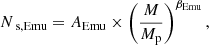
Haloes together with their member galaxies are respectively identified using the friends-of-friends halo finder (Davis et al. 1985) and an improved version of the subhalo finder SUBFIND (Springel et al. 2001) that takes into account the presence of baryons (Dolag et al. 2009). In this work, we mainly focus on a set of 15 simulations labelled Box1a/mr C1–C15 simulations. These span a range of total matter fraction 0.153 < Ωm < 0.428, baryon fraction 0.0408 < Ωb < 0.0504, power spectrum normalisation 0.650 < σ8 < 0.886, and reduced Hubble constant 0.670 < h0 < 0.732, and are chosen using a Latin hypercube sampling (see Sect. 2 in Singh et al. 2020, for more details), as presented in Tables 1 and 2, and are centred around simulation C8, which has WMAP7 cosmological parameters. For each simulation, we study the haloes at a time slice with redshift z = 0.00, 0.14, 0.29, 0.47.
Magneticum simulation specifications used in this work: Box0/mr, Box1a/mr, Box2/hr, and Box4/uhr.
List of Magneticum cosmologies for the Box1a/mr C1–C15 simulations.
In order to study the resolution and mass range of our emulator, we use three additional Magneticum simulations, all with the same WMAP7 cosmology as C8: we use a high-resolution (HR) simulation Box2/hr2 (Hirschmann et al. 2014); we use an ultrahigh-resolution simulation Box4/uhr (Teklu et al. 2015) to study the emulator mass-range validity on low-mass haloes; and a large-volume MR simulation (Box0/mr, Bocquet et al. 2016) in order to validate our high-mass satellite HOD results up to the most massive galaxy clusters of the Universe. We note that the phases of the initial conditions of these three boxes are different.
In this work, all masses and radii are expressed in physical units (except in Table 1 where the units have been chosen differently for the sake of conciseness), and are therefore not implicitly divided by (1 + z) or h0 as in other works on simulations.
3. Comparison of DMO and FP simulations
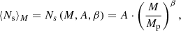
In this section, we describe our motivation to use running FP simulations over multiple cosmologies as opposed to DMO simulations. As we show, the two setups produce mass–richness relations that depend differently on cosmological parameters. Figure 1 shows ⟨Ns⟩M for two cosmologies of which we have the norad counterparts, Box1a/mr C1 and C15, and for two cosmologies of which we have the DMO counterpart, C8 and C1. As DMO and norad simulations have no stars, here we count galaxies based on their total mass MGAL, tot > 1012 M⊙ re-scaled by Ωm/Ωm, WMAP7.
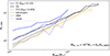 |
Fig. 1. Satellite count Ns, 200c vs. halo mass M200c for Box1a/mr C1 (blue higher lower lines), C8 (black intermediate lines), and C15 (orange lower lines) simulations, their non-radiative (dotted lines, abbreviated with norad) counterpart, and their DMO counterparts (dashed lines). For galaxy masses MSH, tot of greater than 1012 M⊙ × Ωm/Ωm, WMAP7. |
First of all, we note that the C8 DMO Ns − M relation is systematically steeper than the respective FP run. Therefore, these kinds of relations are strongly affected by the presence of baryons. Additionally, we can see that C15 and its norad counterpart have almost the same satellite count, while C1 and its norad counterpart differ by more than a factor of two. Therefore, the effect of baryons on the Ns − M relation depends on cosmological parameters. These two experiments show that studying HOD dependency on non-FP simulations would have produced a different cosmology dependency from the one found in this work.
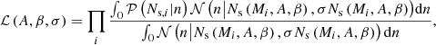
We now test the possibility of recovering the mass–richness relation using the subhalo abundance matching (SHAM) technique. In particular, we perform SHAM based on the subhalo peak of circular velocities estimated at infall (Vpeak), as various works in the literature found this technique to be very effective (see e.g., Chaves-Montero et al. 2016; Hadzhiyska et al. 2021b; Campbell et al. 2018). In order to estimate which cut on Vpeak we should apply to our haloes so that our richness accounts only for well-resolved satellites, we estimated the median value of Vpeak that would provide the same richness of a stellar mass cut of 1011 M⊙ h−1, so that Ns(> Vpeak) = Ns(> 1011 M⊙ h−1). We show the distribution of Vpeak for C15 FP haloes (Mvir > 5 × 10¹⁴ M⊙ h−1) in Fig. 2 and we can see that the median value of Vpeak is approximately 400 s−1 km. We then present our mass–richness results in Fig. 3 (where we applied the same cut as before, so that Vpeak = 400 s−1 km) for FP simulations of C1 and C15 cosmologies and their SHAM counterpart to C15 FP. We note that richness coming from Vpeak-SHAM helps in reproducing abundances across cosmological parameters; however, it systematically over-predicts the C1 SHAM number of satellites (see that the dashed red line lies above the black solid line) because of the different structure number counts in the two cosmologies. From this experiment we conclude that, in order to estimate the mass–richness relation at different cosmologies, running multiple FP simulations (as done in this paper) is more accurate than running DMO simulations and applying SHAM to them.
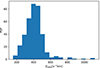 |
Fig. 2. Distribution of Vpeak of C15 haloes needed to obtain the same richness of a stellar mass cut of 1010 M⊙ h−1, so that Ns(> Vpeak) = Ns(> 1011 M⊙ h−1). |
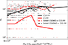 |
Fig. 3. Satellite count with a cut of Vpeak > 400 s−1 km, and richness Ns as a function of the halo mass for FP simulations (solid lines) of C15 (black lines) and C1 (red lines), and for SHAM from their DMO counterpart to C15 FP (dashed lines). |
4. Satellite abundance emulator
In this section, we train an emulator in order to extrapolate the mass–richness relation for some arbitrary cosmological parameters (that are within the range of the parameters of our simulations). We use this emulator in the following section, where we estimate the benefit of using it in mock mass–calibration studies. To this end, we first searched for a stellar-mass cut that causes the richness of Box1a/mr C8 to converge with its high-resolution counterpart Box2b/hr (see Appendix A for more details), and found that if we limit ourselves to galaxies with M⋆ > 2 × 10¹¹ M⊙, then the two simulations have the same mass–richness relations. This relatively high stellar-mass cut could introduce a bias in the satellite population; however, this mass range should still be enough to constrain the normalisation and log-slope of a power-law modelling.
We find that the Box2/hr satellite HOD offset between its fiducial stellar mass cut (1010 M⊙) and the C8 stellar mass cut: (2 × 10¹¹ M⊙) is
 (3)
(3)
We consider this ratio useful to compare MR satellite abundances with HR simulations in the literature with a cut M⋆ > 1010 M⊙.
To estimate the satellite count and compare it consistently between different cosmologies, one must choose a minimum stellar mass cut for each set of cosmological parameters. Following Anbajagane et al. (2020), we decided to rescale the satellite stellar-mass cut with M⋆ > 2 × 10¹¹ M⊙ ⋅ fb/fb, WMAP7. In order to keep the satellite HOD in the power-law regime, we imposed a halo mass cut so that a given mass bin has at least one halo with eight satellites. After this cut, we found that two setups ended with only a few haloes above the mass cut, and so we removed them from further analyses.
4.1. Ns − M relation fit
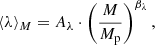
We model the average satellite abundance as a power law of halo mass as in Eq. (2), with a normalisation A and log-slope β as follows
 (4)
(4)
where we use Mp = 5 × 10¹⁴ M⊙ as pivot mass because it approximates the median mass of the haloes selected at z = 0 in the reference cosmology C8.
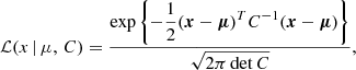
We fit A and β parameters by maximising a likelihood ℒ that models satellite HOD as the convolution of a Poisson and possible deviations from it (as studied in Boylan-Kolchin et al. 2011; Jiang & van den Bosch 2017) with a positive-value Gaussian distribution, with fractional scatter σ on the average satellite abundance. This kind of modelling has been used in mass-calibration studies, such as Costanzi et al. (2019) and Abbott et al. (2020), where the positive-value Gaussian scatter accounts for different accretion histories. The likelihood is calculated as follows:
 (5)
(5)
where i runs over all haloes that we selected in a snapshot.
We maximised3 the likelihood in Eq. (5) for all simulations separately and Fig. 4 shows the power-law fit for C8 and C15 at all available redshifts (left panel) and for all simulations at z = 0 (right panel). The shaded area corresponds to the Gaussian scatter σ, showing that average satellite abundances differ on different cosmologies. We can qualitatively see that different cosmologies and redshift lead to values of β that are close to 1 and a normalisation that can vary by up to a factor of two. See Appendix B for more details on the fit values. We note that C6 cosmology in Fig. 4 has a low normalisation and a larger uncertainty with respect to the other cosmologies. This is because C6 has a relatively low number of satellites, which implies a higher halo mass cut (we remind that this cut is chosen so at least one halo has eight satellites). The consequent small sample size leads to a larger uncertainty. In the following sections, we show that the low richness of C6 may be due to a combination of its low σ8 and Ωb values.
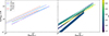 |
Fig. 4. Average satellite count within R200c vs. halo mass for different simulations and redshifts as resulting from maximising the likelihood in Eq. (5). Left panel: satellite count vs. halo mass relation for simulations Box1a/mr C8 (dashed lines) and C15(dotted lines) at three different redshifts (the redder the higher the redshift). Right panel: each line represents a simulation at z = 0, colour coded with green with increasing Ωm; line thickness covers the Gaussian scatter (Poissonian scatter is omitted). |
One may argue that the dependency of Ns on cosmological parameters is rooted in the fact that Ns depends on halo concentration and the halo concentration depends on cosmology. However, even if concentration and assembly bias play a role in the satellite count, this alone cannot account for the dependency between cosmological parameters shown in Fig. 4. In fact, the Box1a/mr C13 simulation has an outstandingly low number of satellites (it has no halo with Ns ≥ 8 and is not included in the emulator), while it does not have a particularly high concentration–mass normalisation (see Fig. 2 in Ragagnin et al. 2021).
In Fig. 5, we summarise the parameters A, β, and σ found by maximising Eq. (5) for Δ200c, where we can see a mild redshift evolution of A and β as found in Kravtsov et al. (2004). An increase in Ns with redshift could be expected, because towards high redshift we are selecting an increasing number of young clusters (the mass cut does not change with redshift), and young clusters are known to be richer (see Bose et al. 2019).
 |
Fig. 5. Fit parameters of Eqs. (4) and (5) for Ns, 200c. From left to right, parameters A, B, and σ as a function of Ωm, and colour coded by 1 + z (the redder, the higher the redshift). Vertical error bars corresponds to the uncertainty given from the likelihood posterior in Eq. (5). |
4.2. The Gaussian process regression emulator
In order to model the HOD as a function of cosmological parameters and redshift, we build an emulator based on Gaussian process regression (GPR) with the aim of predicting A, β, and σ. Our main motivation is that these parameters do not follow simple functional forms, such as a power law, as can be seen in Fig. 5.
For this purpose, we train the GPR model4 on an array of Ai, βi, and σi residuals with respect to a power-law fit on cosmological parameters (where i runs in all setups). We present fit posteriors in Appendix C, and below we report the results and errors from the fit:
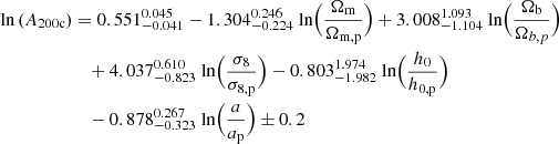 (6)
(6)
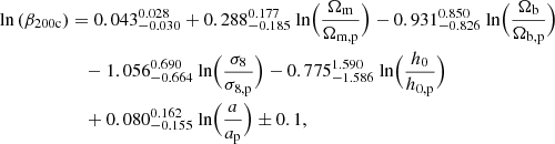 (7)
(7)
where pivot cosmology parameters are set to C8 values and pivot scale factor is a = 0.87.
We trained our emulator on log-scaled values, as follows:
![Mathematical equation: $$ \begin{aligned} {\left\{ \begin{array}{ll} X_i=\Bigg [ \text{ ln}\Big (\dfrac{\Omega _{\mathrm{m},i}}{\Omega _{\rm m,p}}\Big ), \text{ ln}\Big (\dfrac{\Omega _{\mathrm{b},i}}{\Omega _{\rm b,p}}\Big ), \text{ ln}\Big (\dfrac{\sigma _{8,i}}{\sigma _{\rm 8,p}}\Big ), \text{ ln}\Big (\dfrac{h_{0,i}}{h_{\rm 0,p}}\Big ), \text{ ln}\Big (\dfrac{1+z_{\rm p}}{1+z_i}\Big ) \Bigg ]\\ \\ { y}_i=\Bigg [ \text{ ln}\Big (\dfrac{A_i}{A_\Delta }\Big ), \text{ ln}\Big (\dfrac{\beta _i}{\beta _\Delta }\Big ), \text{ ln}\Big (\dfrac{\sigma _i}{\sigma _\Delta }\Big ) \Bigg ]\ , \end{array}\right.} \end{aligned} $$](/articles/aa/full_html/2023/07/aa42392-21/aa42392-21-eq10.gif) (8)
(8)
where X = {Xi} is the input data; y = {yi} the output data; i runs over all data points (i.e., all selected snapshots) for which we maximised the likelihood in Eq. (5); AΔ, βΔ, and σΔ are a function of cosmology; and, as pivot values, we used the same as in Eqs. (6) and (7).
Concerning the GPR model, we modelled our kernel K as a constant K0 times a Gaussian radial basis function kernel with length scale l:
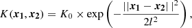 (9)
(9)
where the norm ∥⋯∥ is the euclidean distance.
We maximised the log marginal likelihood as proposed in Eq. (2.30) in Rasmussen & Williams (2005) and allowed parameters K0 and l to vary in the maximisation. Hereafter, we define the Emulator predictions as AEmu, βEmu, which themselves depends on a cosmology and scale factor (Ωm, Ωb, σ8, h0, a). We define the emulated average number of satellites Ns, Emu as
 (10)
(10)
where AEmu and βEmu are predicted by our emulator and depend on cosmology and redshift.
4.3. Emulator error estimate
To estimate the precision of our emulator, we use the same technique as used by Bocquet et al. (2020): for each data vector available (Xi, yi), we (i) build a predictor trained on the complete data-set except that point (i.e., [X, Y]i = [{X}\Xi, {Y}\yi]), hereafter OEmu, i, and (ii) for each predictor we compute its relative error in predicting the untrained value yi. To contextualise the relative error of the emulator, we compare it with the relative error obtained by predicting yi using only the average of all values (thus ignoring any cosmology dependency).
As we can see in Fig. 6, the residual PDF of the A from the emulator (top panel, orange steps) is much more peaked around 1 than the PDF from the predictor based on the averages (blue steps). This implies that the emulator is effective in predicting mass–richness normalisation A. On the other hand, there is no significant gain in recovering the log-slope β.
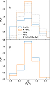 |
Fig. 6. PDF of residuals for predictor Pi = Emui and the residual based on predictions from the average values (Pi = ⟨Y⟩), with respect to the missing data point yi. Data are computed on overdensity Δ200c. The upper row shows the PDF for yi = Ai (normalisation), and the lower row shows the PDF for yi = βi (log-slope). The scatter obtained with the emulator is significantly smaller than the residuals on average. Grey lines correspond to the residuals when the emulator is trained without either σ8 (dotted line), h0 (dashed line), or when using Ωb/Ωm instead of training it with Ωb and Ωm separately (dash-dotted line). |
The residuals distribution of the emulator within Δ200c corresponds to a precision of ≈10 − 20%, and the average of the GPR error estimations in the missing points is of the same order of magnitude, and therefore the emulator is capable of correctly predicting its own uncertainty.
Finally, we study whether we need to train our HOD emulator with the four cosmological parameters Ωm, Ωb, σ8, and h0 or we can reach the same precision by dropping some of these parameters. For this reason, in Fig. 6, we show the residuals of the emulator trained without σ8 (dotted line) or without h0 (dashed line) by using Ωb/Ωm instead of training on Ωb and Ωm separately (dash-dotted line). We find that in all these scenarios, the residuals of the predictions are larger than the complete setup, which motivates us to use all parameters.
4.4. Mass range
In this subsection, we test the mass range validity of our satellite HOD across various orders of magnitude in order to identify the halo mass range of it.
Figure 7 shows that the same power-law satellite abundance holds from the most massive galaxy clusters M200c ≈ 6 × 10¹⁵ M⊙ down to haloes of M200c ≈ 5 × 10¹³ M⊙. It is at this mass that the low-mass drop of the M⋆ > 1010 M⊙ cut starts, which is particularly visible in the Box4/uhr regime haloes. Both Box0/mr and C8 satellite abundances are rescaled using Eq. (3). We estimated the fractional difference between the average Ns value estimated using the emulator and that from Magneticum boxes (Box0/mr, Box2/hr, Box4/uhr) and find that, on average, the relative difference is ≈5%. This shows that Eq. (3) holds between richness values from boxes with varying resolutions.
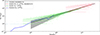 |
Fig. 7. Satellite count Ns, 200c vs. halo mass M200c for three Magneticum simulations, Box4/uhr (blue coloured and moved slightly down to improve readability), Box2/hr (green coloured), and Box0/mr (red colour) to account for resolution effects. Data points represent single haloes and coloured lines represent average values per mass bin. The black line is the emulator prediction, and the shaded area corresponds to the relative uncertainty from Poisson distribution. Emulator and Box0/mr data are rescaled with Eq. (3). |
Finally, we study how each cosmological parameter affects the Ns − M relation. Figure 8 shows the variation of parameters A and B as a function of the fractional variation of each cosmological parameter – namely Ωm, Ωb, σ8, h0, and scale factor – separately around WMAP7 values. We also note that the decrease in the normalisation with decreasing σ8 and Ωb is in agreement with the low mass–richness normalisation of C6 cosmology.
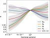 |
Fig. 8. Variation of Ns, 200c emulator A, β, and σ as a function of fractional variation of cosmological parameters Ωm, Ωb, σ8, h0, and scale factor. Shaded areas show 1 standard deviation provided by the Gaussian process error estimation. |
5. Impact on mock observations
In this section, we test the cosmology-dependence of the HOD on mock catalogues in order to estimate its impact on the cosmological parameter constraints. To this purpose, we consider the richness, which is a weighted sum of the galaxy members often used as a mass proxy in cluster surveys driven by photometric data. We recast Eq. (4) in terms of a richness–mass relation:
 (11)
(11)
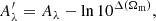
with Aλ = A0 ⋅ Aemu = 72.4 ± 0.7 and βλ = β0 ⋅ βemu = 0.935 ± 0.038 (from table IV of Costanzi et al. 2021). Here, Aemu and βemu are the predictions of the emulator and contain the dependence on cosmology, while A0 and β0 represent the cosmology-independent part of the total parameters.
To perform the analysis, we extract a catalogue of halo masses corresponding to the C8 simulation at redshift z = 0, following the Despali et al. (2016) analytical mass function. This step ensures that we have a proper description of the mass function, which we use to obtain an unbiased estimation of parameters. We obtain a catalogue with ∼2.8 × 10⁵ objects, with virial masses above Mvir > 1013 M⊙, to which we assign richness by applying Eq. (11) plus a Poisson scatter. To ease the analysis, we neglect the intrinsic scatter of the HOD, which is subdominant with respect the Poisson one. In the end, we compute the number counts by considering five richness bins in the range λ = 30 − 300, where the sample is complete in mass.
We then maximise a Gaussian likelihood:
 (12)
(12)
where x is the mock ‘observed’ number count, μ is the count from a Monte Carlo Markov chain (MCMC) likelihood maximisation, and C is the covariance matrix computed following the analytical model of Hu & Kravtsov (2003). As in this test we only aim to give an estimation of the impact of the cosmology-dependent HOD, we run a simplified MCMC process with only two free cosmological parameters, Ωm and log10As (and thus σ8), neglecting the dependence of the HOD on Ωb and h0, and neglecting the redshift dependence. Following the approach of Singh et al. (2020), we compare three different cases below.
Case no cosmo: We ignore the cosmology dependence of the HOD so that Aλ = A0 and βλ = β0 and we assume flat uninformative priors both on Ωm and log10As and on Aλ and βλ.
Case cosmo: We assume flat uninformative priors on Ωm, log10As, A0, and β0, plus Gaussian priors on Aλ and βλ, respectively, given by 𝒩(72.4, 7.0) and 𝒩(0.935, 0.038). The cosmology-dependent parameters Aemu and βemu are computed by the emulator at each step of the MCMC process, and, to take into account the emulator inaccuracy, we randomly extract a value from a Gaussian distribution with its centre in the emulator prediction and amplitude equal to σ log Aemu = 0.06 and σ log βemu = 0.09.
Case cosmo + WL: we add the weak lensing (WL) cosmological dependence – which affects the mass calibration in the real observations – to figure out whether or not the combination of the cosmology-dependent HOD and other cosmological probes could improve the parameter constraints. We model the dependence by modifying the prior on Aλ, which becomes a Gaussian prior with the same amplitude as the previous case, but centred on
 (13)
(13)
with 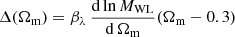 , where
 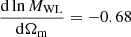 is the average value from Table I of Costanzi et al. (2019).
In Fig. 9, we show the posterior distributions resulting from the three analyses. As expected, the marginalised posteriors recovered by the cosmo case are similar to the ones from the no cosmo case, but in addition the former is able to constrain the cosmology-dependent and cosmology-independent components of the richness–mass relation separately. This can be an advantage, because the components of Aλ show a stronger degeneracy with cosmological parameters with respect to the one shown by Aλ alone. This degeneracy can be exploited when combined with other cosmological probes. On the contrary, this decomposition for βλ does not present the same advantage, as the full parameter has a higher degeneracy with cosmological parameters than its components do.
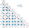 |
Fig. 9. Contour plots at 68 and 95% confidence level for the three cases described in Sect. 5: no cosmo (black), cosmo (blue), and cosmo + WL (red) contours. The grey dashed lines represent the input values of parameters. |
The third case presents similar posteriors to the simple cosmo case; to better compare the differences, we quantify the accuracy of the parameter estimation by computing the figure of merit (FoM; Albrecht et al. 2006):
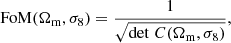 (14)
(14)
where C(Ωm, σ8) is the parameter covariance matrix obtained from the posteriors. The FoM is proportional to the inverse of the area enclosed by the ellipse representing the 68% confidence level: the higher the FoM, the more accurate the parameter evaluation. The result, shown in Table 3, indicates that the use of the cosmology-dependent HOD allows us to obtain posteriors that have greater constraining power, and that are further improved by the addition of the WL information. To prove that the cosmo + WL result is not achieved only thanks to the addition of WL, we also show the FoM for the no cosmo + WL case, which has a constraining power similar to the simple no cosmo case. By comparing the FoM of the three cases, we obtain an improvement of about 6% for the cosmo case and of about 11% for the cosmo + WL case with respect to the no cosmo case.
6. Conclusions
We tackled the problem of studying the dependency of the satellite count–halo mass relationship on cosmological parameters and redshift and studied how modelling could improve observational studies designed to obtain mass calibrations using mass–richness relations. To this end, we used FP Magneticum simulations Box1a C1–C15 (see Table 1), which were run with the same initial conditions but different cosmological parameters, namely Ωm, Ωb, σ8, and h0. We did not recalibrate feedback parameters over the various runs, and in this study we focus on the effect of cosmological parameters on the high-mass satellite abundance Ns for a fixed feedback configuration. Our main findings can be summarised as follows:
-
We show that DMO and FP subhaloes have different dependencies on cosmological parameters, showing the importance of parametrising mass–richness relations with results from FP simulations rather than DMO ones.
-
We built an emulator capable of predicting normalisation, log-slope, and log-scatter of the high-mass power-law regime of the N − M relation based on GPR modelling in order to predict the number of satellites for a given cosmology. We estimate its error to be ≈20%. This error is comparable to the same uncertainty predicted by the GPR, which shows that the GPR learned to extract mean values as well as their associated uncertainties.
-
We tested whether or not parametrising the mass–richness relation with cosmological parameters can improve mass-calibration studies. The likelihood analysis on mock mass-calibration showed that the use of a cosmology-dependent HOD provides an improvement (∼5%) in the constraining power over a simple cosmology-independent HOD, which can be further improved (∼10%) if combined with multiple mass proxies, such as the weak lensing signal.
This study was carried out over a small number of cosmologies and with a resolution limited to the high-mass regime of haloes. It shows that mass-calibrations can benefit from modelling mass–richness relations with cosmological parameters from hydro-simulations. Future studies could focus on the dependency of the radial distribution of substructures on cosmology. The emulator log-slope predictions have a large uncertainty (see Fig. 8 where the shaded area spans β ∈ [0.9, 1]), which means there is a need for simulations that consider additional cosmological parameters and feedback parameters in order to improve GPR interpolation.
Box2/hr halo data are available at the web portal presented in Ragagnin et al. (2017).
We used python package emcee from Foreman-Mackey et al. (2019).
We used sklearn package (Pedregosa et al. 2011).
Acknowledgments
The Magneticum Pathfinder simulations were partially performed at the Leibniz-Rechenzentrum with CPU time assigned to the Project ‘pr86re’. A.F. would like to thank Stefano Borgani for useful discussions. A.R. is supported by the EuroEXA project (grant no. 754337). K.D. acknowledges support by DAAD contract number 57396842. A.R. acknowledges support by MIUR-DAAD contract number 34843 “The Universe in a Box”. A.S., A.F. and P.S. are supported by the ERC-StG ‘ClustersXCosmo’ grant agreement 716762. A.S. is supported by the FARE-MIUR grant ‘ClustersXEuclid’ R165SBKTMA and INFN InDark Grant. This work was supported by the Deutsche Forschungsgemeinschaft (DFG, German Research Foundation) under Germany’s Excellence Strategy – EXC-2094 – 390783311. K.D. acknowledges funding for the COMPLEX project from the European Research Council (ERC) under the European Union’s Horizon 2020 research and innovation program grant agreement ERC-2019-AdG 860744. A.R. acknowledges support from the grant PRIN-MIUR 2017 WSCC32. We are especially grateful for the support by M. Petkova through the Computational Center for Particle and Astrophysics (C2PAP). Information on the Magneticum Pathfinder project is available at http://www.magneticum.org.
References
- Abbott, T. M. C., Aguena, M., Alarcon, A., et al. 2020, Phys. Rev. D, 102, 023509 [Google Scholar]
- Albrecht, A., Bernstein, G., Cahn, R., et al. 2006, arXiv e-prints [arXiv:astro-ph/0609591] [Google Scholar]
- Anbajagane, D., Evrard, A. E., Farahi, A., et al. 2020, MNRAS, 495, 686 [NASA ADS] [CrossRef] [Google Scholar]
- Avila, S., Gonzalez-Perez, V., Mohammad, F. G., et al. 2020, MNRAS, 499, 5486 [NASA ADS] [CrossRef] [Google Scholar]
- Beck, A. M., Murante, G., Arth, A., et al. 2016, MNRAS, 455, 2110 [Google Scholar]
- Biffi, V., Dolag, K., & Böhringer, H. 2013, MNRAS, 428, 1395 [Google Scholar]
- Bocquet, S., Saro, A., Dolag, K., & Mohr, J. J. 2016, MNRAS, 456, 2361 [Google Scholar]
- Bocquet, S., Heitmann, K., Habib, S., et al. 2020, ApJ, 901, 5 [Google Scholar]
- Bose, S., Eisenstein, D. J., Hernquist, L., et al. 2019, MNRAS, 490, 5693 [CrossRef] [Google Scholar]
- Boylan-Kolchin, M., Springel, V., White, S. D. M., Jenkins, A., & Lemson, G. 2009, MNRAS, 398, 1150 [Google Scholar]
- Boylan-Kolchin, M., Bullock, J. S., & Kaplinghat, M. 2011, MNRAS, 415, L40 [NASA ADS] [CrossRef] [Google Scholar]
- Campbell, D., van den Bosch, F. C., Padmanabhan, N., et al. 2018, MNRAS, 477, 359 [Google Scholar]
- Castro, T., Borgani, S., Dolag, K., et al. 2021, MNRAS, 500, 2316 [Google Scholar]
- Chaves-Montero, J., Angulo, R. E., Schaye, J., et al. 2016, MNRAS, 460, 3100 [NASA ADS] [CrossRef] [Google Scholar]
- Costanzi, M., Rozo, E., Simet, M., et al. 2019, MNRAS, 488, 4779 [NASA ADS] [CrossRef] [Google Scholar]
- Costanzi, M., Saro, S., Bocquet, T. M., et al. 2021, Phys. Rev. D, 103, 043522P [NASA ADS] [CrossRef] [Google Scholar]
- Coupon, J., Arnouts, S., van Waerbeke, L., et al. 2015, MNRAS, 449, 1352 [NASA ADS] [CrossRef] [Google Scholar]
- Davis, M., Efstathiou, G., Frenk, C. S., & White, S. D. M. 1985, ApJ, 292, 371 [Google Scholar]
- Despali, G., & Vegetti, S. 2017, MNRAS, 469, 1997 [NASA ADS] [CrossRef] [Google Scholar]
- Despali, G., Giocoli, C., Angulo, R. E., et al. 2016, MNRAS, 456, 2486 [NASA ADS] [CrossRef] [Google Scholar]
- Dolag, K., Borgani, S., Murante, G., & Springel, V. 2009, MNRAS, 399, 497 [Google Scholar]
- Dolag, K., Gaensler, B. M., Beck, A. M., & Beck, M. C. 2015, MNRAS, 451, 4277 [NASA ADS] [CrossRef] [Google Scholar]
- Dolag, K., Komatsu, E., & Sunyaev, R. 2016, MNRAS, 463, 1797 [Google Scholar]
- Fabjan, D., Borgani, S., Tornatore, L., et al. 2010, MNRAS, 401, 1670 [Google Scholar]
- Ferland, G. J., Korista, K. T., Verner, D. A., et al. 1998, PASP, 110, 761 [Google Scholar]
- Foreman-Mackey, D., Farr, W. M., Sinha, M., et al. 2019, J. Open Source Softw., 4, 1864 [NASA ADS] [CrossRef] [Google Scholar]
- Giocoli, C., Tormen, G., & van den Bosch, F. C. 2008, MNRAS, 386, 2135 [NASA ADS] [CrossRef] [Google Scholar]
- Guzik, J., & Seljak, U. 2002, MNRAS, 335, 311 [CrossRef] [Google Scholar]
- Hadzhiyska, B., Bose, S., Eisenstein, D., & Hernquist, L. 2021a, MNRAS, 501, 1603 [Google Scholar]
- Hadzhiyska, B., Tacchella, S., Bose, S., & Eisenstein, D. J. 2021b, MNRAS, 502, 3599 [NASA ADS] [CrossRef] [Google Scholar]
- Hearin, A. P., Zentner, A. R., van den Bosch, F. C., Campbell, D., & Tollerud, E. 2016, MNRAS, 460, 2552 [NASA ADS] [CrossRef] [Google Scholar]
- Hirschmann, M., Dolag, K., Saro, A., et al. 2014, MNRAS, 442, 2304 [Google Scholar]
- Hu, W., & Kravtsov, A. V. 2003, ApJ, 584, 702 [Google Scholar]
- Jiang, F., & van den Bosch, F. C. 2017, MNRAS, 472, 657 [NASA ADS] [CrossRef] [Google Scholar]
- Kravtsov, A. V., Berlind, A. A., Wechsler, R. H., et al. 2004, ApJ, 609, 35 [Google Scholar]
- Leauthaud, A., Saito, S., Hilbert, S., et al. 2017, MNRAS, 467, 3024 [Google Scholar]
- Pedregosa, F., Varoquaux, G., Gramfort, A., et al. 2011, J. Mach. Learn. Res., 12, 2825 [Google Scholar]
- Ragagnin, A., Tchipev, N., Bader, M., Dolag, K., & Hammer, N. J. 2016, in Advances in Parallel Computing, Volume 27: Parallel Computing: On the Road to Exascale, eds. G. R. Joubert, H. Leather, M. Parsons, F. Peters, & M. Sawyer (IOP Ebook), 411 [Google Scholar]
- Ragagnin, A., Dolag, K., Biffi, V., et al. 2017, Astron. Comput., 20, 52 [Google Scholar]
- Ragagnin, A., Dolag, K., Moscardini, L., Biviano, A., & D’Onofrio, M. 2019, MNRAS, 486, 4001 [Google Scholar]
- Ragagnin, A., Saro, A., Singh, P., & Dolag, K. 2021, MNRAS, 500, 5056 [Google Scholar]
- Rasmussen, C. E., & Williams, C. K. I. 2005, Gaussian Processes for Machine Learning (Adaptive Computation and Machine Learning) (The MIT Press) [Google Scholar]
- Reid, B. A., Seo, H.-J., Leauthaud, A., Tinker, J. L., & White, M. 2014, MNRAS, 444, 476 [NASA ADS] [CrossRef] [Google Scholar]
- Remus, R.-S., Dolag, K., Naab, T., et al. 2017, MNRAS, 464, 3742 [Google Scholar]
- Rodríguez-Puebla, A., Primack, J. R., Avila-Reese, V., & Faber, S. M. 2017, MNRAS, 470, 651 [Google Scholar]
- Ross, A. J., Percival, W. J., & Brunner, R. J. 2010, MNRAS, 407, 420 [CrossRef] [Google Scholar]
- Saro, A., Liu, J., Mohr, J. J., et al. 2014, MNRAS, 440, 2610 [Google Scholar]
- Singh, P., Saro, A., Costanzi, M., & Dolag, K. 2020, MNRAS, 494, 3728 [NASA ADS] [CrossRef] [Google Scholar]
- Skibba, R. A. 2009, MNRAS, 392, 1467 [CrossRef] [Google Scholar]
- Springel, V. 2005, MNRAS, 364, 1105 [Google Scholar]
- Springel, V., White, S. D. M., Tormen, G., & Kauffmann, G. 2001, MNRAS, 328, 726 [Google Scholar]
- Springel, V., Di Matteo, T., & Hernquist, L. 2005a, MNRAS, 361, 776 [Google Scholar]
- Springel, V., White, S. D. M., Jenkins, A., et al. 2005b, Nature, 435, 629 [Google Scholar]
- Steinborn, L. K., Dolag, K., Hirschmann, M., Prieto, M. A., & Remus, R.-S. 2015, MNRAS, 448, 1504 [Google Scholar]
- Steinborn, L. K., Dolag, K., Comerford, J. M., et al. 2016, MNRAS, 458, 1013 [Google Scholar]
- Teklu, A. F., Remus, R.-S., Dolag, K., et al. 2015, ApJ, 812, 29 [Google Scholar]
- Tornatore, L., Borgani, S., Dolag, K., & Matteucci, F. 2007, MNRAS, 382, 1050 [Google Scholar]
- van den Bosch, F. C., Yang, X., Mo, H. J., & Norberg, P. 2005, MNRAS, 356, 1233 [CrossRef] [Google Scholar]
- Voivodic, R., & Barreira, A. 2021, JCAP, 05, 069 [Google Scholar]
- Wang, J., De Lucia, G., Kitzbichler, M. G., & White, S. D. M. 2008, MNRAS, 384, 1301 [CrossRef] [Google Scholar]
- Wang, E., Wang, H., Mo, H., et al. 2018, ApJ, 864, 51 [NASA ADS] [CrossRef] [Google Scholar]
- Wechsler, R. H., & Tinker, J. L. 2018, ARA&A, 56, 435 [NASA ADS] [CrossRef] [Google Scholar]
- Yuan, S., Hadzhiyska, B., Bose, S., Eisenstein, D. J., & Guo, H. 2021, MNRAS, 502, 3582 [NASA ADS] [CrossRef] [Google Scholar]
- Zenteno, A., Mohr, J. J., Desai, S., et al. 2016, MNRAS, 462, 830 [NASA ADS] [CrossRef] [Google Scholar]
Appendix A: Stellar mass cut
To build our HOD emulator, first of all we estimate which stellar mass cut to apply to the satellite count of our Box1a/mr C1–C15 simulations. For this purpose, we vary the stellar mass cut of both C8 and its HR counterpart (Box2/hr) until their Ns − M relations statistically match. Figure A.1 shows convergence tests for stellar mass of C8 satellites. The left panel shows the Ns − M relation of C8 and Box2/hr with the fiducial Box2/hr mass cut M⋆ > 1010M⊙ (as chosen in Anbajagane et al. 2020); the central panel shows that a stellar mass cut M⋆ > 1011M⊙ is not high enough to make C8 match its HR counterpart; the right panel shows that a stellar mass cut M⋆ > 2 ⋅ 1011M⊙ is capable of reconciling the two simulations.
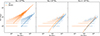 |
Fig. A.1. Galaxy abundance of HR (Box2/hr in orange) and MR (C8 in blue) simulations for varying minimum stellar mass of galaxies: M⋆ > 1010M⊙ (left panel), M⋆ > 1011M⊙ (middle panel), and M⋆ > 2 ⋅ 1010M⊙ (right panel). |
Appendix B: Satellite abundance fit for each simulation
Table B.1 reports the fit parameters of average satellite abundance as a function of halo mass, for all setups that had a p−value below 0.9 and higher than 0.01. The problematic fits were those at z = 0.67, where a few of them failed, which is probably because the resolution of our simulations is not always enough to reach this redshift. Only a total of 48 fits were successful.
Values of the halo mass cut (Mcut in units of 1014 M⊙), and mass–richness fit parameters lnA, β, and σ (as in of Eq. 4) for each simulation used in this work.
In order to fit the power-law halo-mass region of the satellite abundance relation, we imposed a halo mass cut at Mvir = 3 ⋅ 1014 M⊙ for C8 simulation and scaled the mass cut to other simulations according to their baryon fraction. Some cuts were modified in order to manually shrink or enlarge the halo range so as to maximise the number of data points and yet not cross the mass cut at low halo masses.
Figure B.1 shows the posterior of the fit for simulation Box1a/mr C8 z = 0. Here we can see that the fractional scatter σ is consistent with zero.
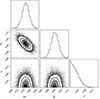 |
Fig. B.1. Posterior associated to likelihood (5) for Box1a/mr C8 at z = 0 for Δ= 200c. Parameters A and β are as in Eq. (4) and σ is the fractional scatter in the likelihood. |
Appendix C: Cosmology-dependent power-law fit posteriors
In this Appendix, we report the results of the A200c fit. To fit A200c and similarly also β and σ for both Δ200c and Δvir, as in Eqs. (6) and (7), we maximised a likelihood as follows:
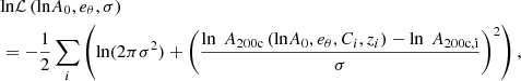 (C.1)
(C.1)
where i runs over all setups, Ci and zi are the cosmology and redshift of that setup, A200c, i is the normalisation found in Sect. 4 for a given setup, eθ is a set of exponents (em, eb, eσ, eh, ea) for the respective input parameters θi = (Ci, ai) = (Ωm, i, Ωb, i, σ8, i, h0, i, ai), where σ is the fractional scatter, and A200c has a power-law dependency from cosmological parameters, as follows:
 (C.2)
(C.2)
where the pivot values θi, p are presented in Sect. 4.2. Figure C.1 shows an example of a posterior distribution of parameters (lnA0, eθ, σ) for a single snapshot. The evaluation of β200c, σ200c, Avir, βvir and σ200c was performed in the same way as described above.
 |
Fig. C.1. Posterior associated to the likelihood in Eq. (5). The parameter lnA0 is the normalisation |

All Tables
Magneticum simulation specifications used in this work: Box0/mr, Box1a/mr, Box2/hr, and Box4/uhr.
Values of the halo mass cut (Mcut in units of 1014 M⊙), and mass–richness fit parameters lnA, β, and σ (as in of Eq. 4) for each simulation used in this work.
All Figures
|
Fig. 1. Satellite count Ns, 200c vs. halo mass M200c for Box1a/mr C1 (blue higher lower lines), C8 (black intermediate lines), and C15 (orange lower lines) simulations, their non-radiative (dotted lines, abbreviated with norad) counterpart, and their DMO counterparts (dashed lines). For galaxy masses MSH, tot of greater than 1012 M⊙ × Ωm/Ωm, WMAP7. |
| In the text | |
|
Fig. 2. Distribution of Vpeak of C15 haloes needed to obtain the same richness of a stellar mass cut of 1010 M⊙ h−1, so that Ns(> Vpeak) = Ns(> 1011 M⊙ h−1). |
| In the text | |
|
Fig. 3. Satellite count with a cut of Vpeak > 400 s−1 km, and richness Ns as a function of the halo mass for FP simulations (solid lines) of C15 (black lines) and C1 (red lines), and for SHAM from their DMO counterpart to C15 FP (dashed lines). |
| In the text | |
|
Fig. 4. Average satellite count within R200c vs. halo mass for different simulations and redshifts as resulting from maximising the likelihood in Eq. (5). Left panel: satellite count vs. halo mass relation for simulations Box1a/mr C8 (dashed lines) and C15(dotted lines) at three different redshifts (the redder the higher the redshift). Right panel: each line represents a simulation at z = 0, colour coded with green with increasing Ωm; line thickness covers the Gaussian scatter (Poissonian scatter is omitted). |
| In the text | |
|
Fig. 5. Fit parameters of Eqs. (4) and (5) for Ns, 200c. From left to right, parameters A, B, and σ as a function of Ωm, and colour coded by 1 + z (the redder, the higher the redshift). Vertical error bars corresponds to the uncertainty given from the likelihood posterior in Eq. (5). |
| In the text | |
|
Fig. 6. PDF of residuals for predictor Pi = Emui and the residual based on predictions from the average values (Pi = ⟨Y⟩), with respect to the missing data point yi. Data are computed on overdensity Δ200c. The upper row shows the PDF for yi = Ai (normalisation), and the lower row shows the PDF for yi = βi (log-slope). The scatter obtained with the emulator is significantly smaller than the residuals on average. Grey lines correspond to the residuals when the emulator is trained without either σ8 (dotted line), h0 (dashed line), or when using Ωb/Ωm instead of training it with Ωb and Ωm separately (dash-dotted line). |
| In the text | |
|
Fig. 7. Satellite count Ns, 200c vs. halo mass M200c for three Magneticum simulations, Box4/uhr (blue coloured and moved slightly down to improve readability), Box2/hr (green coloured), and Box0/mr (red colour) to account for resolution effects. Data points represent single haloes and coloured lines represent average values per mass bin. The black line is the emulator prediction, and the shaded area corresponds to the relative uncertainty from Poisson distribution. Emulator and Box0/mr data are rescaled with Eq. (3). |
| In the text | |
|
Fig. 8. Variation of Ns, 200c emulator A, β, and σ as a function of fractional variation of cosmological parameters Ωm, Ωb, σ8, h0, and scale factor. Shaded areas show 1 standard deviation provided by the Gaussian process error estimation. |
| In the text | |
|
Fig. 9. Contour plots at 68 and 95% confidence level for the three cases described in Sect. 5: no cosmo (black), cosmo (blue), and cosmo + WL (red) contours. The grey dashed lines represent the input values of parameters. |
| In the text | |
|
Fig. A.1. Galaxy abundance of HR (Box2/hr in orange) and MR (C8 in blue) simulations for varying minimum stellar mass of galaxies: M⋆ > 1010M⊙ (left panel), M⋆ > 1011M⊙ (middle panel), and M⋆ > 2 ⋅ 1010M⊙ (right panel). |
| In the text | |
|
Fig. B.1. Posterior associated to likelihood (5) for Box1a/mr C8 at z = 0 for Δ= 200c. Parameters A and β are as in Eq. (4) and σ is the fractional scatter in the likelihood. |
| In the text | |
|
Fig. C.1. Posterior associated to the likelihood in Eq. (5). The parameter lnA0 is the normalisation |
| In the text | |
Current usage metrics show cumulative count of Article Views (full-text article views including HTML views, PDF and ePub downloads, according to the available data) and Abstracts Views on Vision4Press platform.
Data correspond to usage on the plateform after 2015. The current usage metrics is available 48-96 hours after online publication and is updated daily on week days.
Initial download of the metrics may take a while.