| Issue |
A&A
Volume 675, July 2023
|
|
|---|---|---|
| Article Number | A202 | |
| Number of page(s) | 21 | |
| Section | Cosmology (including clusters of galaxies) | |
| DOI | https://doi.org/10.1051/0004-6361/202039293 | |
| Published online | 20 July 2023 | |
Clustering of red sequence galaxies in the fourth data release of the Kilo-Degree Survey
1
Leiden Observatory, Leiden University, PO Box 9513 Leiden 2300 RA, The Netherlands
e-mail: This email address is being protected from spambots. You need JavaScript enabled to view it.
2
Center for Theoretical Physics, Polish Academy of Sciences, Al. Lotników 32/46, 02-66 Warsaw, Poland
3
Ruhr-Universität Bochum, Astronomisches Institut (AIRUB), German Centre for Cosmological Lensing, Universitätsstr. 150, 44801 Bochum, Germany
4
Institute for Astronomy, University of Edinburgh, Royal Observatory, Blackford Hill, Edinburgh EH9 3HJ, UK
5
School of Physics, Monash University, Clayton, VIC 3800, Australia
6
Argelander-Institut für Astronomie, Universität Bonn, Auf dem Hügel 71, 53121 Bonn, Germany
7
Department of Physics and Astronomy, University College London, Gower Street, London WC1E 6BT, UK
8
Department of Physics, University of Oxford, Denys Wilkinson Building, Keble Road, Oxford OX1 3RH, UK
9
Department of Astrophysical Sciences, Princeton University, 4 Ivy Lane, Princeton, NJ 08544, USA
Received:
30
August
2020
Accepted:
10
February
2023
Abstract
We present a sample of luminous red sequence galaxies as the basis for a study of the large-scale structure in the fourth data release of the Kilo-Degree Survey. The selected galaxies are defined by a red sequence template, in the form of a data-driven model of the colour-magnitude relation conditioned on redshift. In this work, the red sequence template was built using the broad-band optical+near infrared photometry of KiDS-VIKING and the overlapping spectroscopic data sets. The selection process involved estimating the red sequence redshifts, assessing the purity of the sample and estimating the underlying redshift distributions of redshift bins. After performing the selection, we mitigated the impact of survey properties on the observed number density of galaxies by assigning photometric weights to the galaxies. We measured the angular two-point correlation function of the red galaxies in four redshift bins and constrain the large-scale bias of our red sequence sample assuming a fixed ΛCDM cosmology. We find consistent linear biases for two luminosity-threshold samples (‘dense’ and ‘luminous’). We find that our constraints are well characterised by the passive evolution model.
Key words: galaxies: distances and redshifts / large-scale structure of Universe / methods: data analysis / methods: statistical
© The Authors 2023
 Open Access article, published by EDP Sciences, under the terms of the Creative Commons Attribution License (https://creativecommons.org/licenses/by/4.0), which permits unrestricted use, distribution, and reproduction in any medium, provided the original work is properly cited.
This article is published in open access under the Subscribe to Open model. This email address is being protected from spambots. You need JavaScript enabled to view it. to support open access publication.
1. Introduction
The Kilo-Degree Survey (KiDS) is an optical galaxy survey primarily designed to map the large-scale structure by studying the weak gravitational lensing of galaxies (de Jong et al. 2013; Kuijken et al. 2015, 2019). This is done by measuring the distortion of the shapes of distant galaxies known as cosmic shear, which has become a cornerstone of modern cosmological imaging surveys. Current surveys such as the Dark Energy Survey (DES)1, Hyper Suprime Cam Subaru Strategic Program (HSC)2, and KiDS3 are already yielding competitive constraints on certain cosmological parameters using weak gravitational lensing (e.g. Troxel et al. 2018; Hikage et al. 2019; Hildebrandt et al. 2020; Asgari et al. 2021).
However, the full potential of large imaging surveys such as KiDS can be realised by constructing a galaxy sample with robust redshift estimates which can be utilised for a wide array of applications, such as studying intrinsic alignments and galaxy-dark matter connection, as well as setting cosmological constraints that are complementary to cosmic shear analyses.
In this work, we focus on selecting a sample of red sequence galaxies with robust redshift estimates as well as measuring their angular two-point correlation function in slices of redshift. Following the work of Vakili et al. (2019), we constructed a sample of red sequence galaxies by leveraging the fact that the distribution of these galaxies in colour space follows a multivariate Gaussian distribution. The mean of this distribution is a linear function of magnitude. Furthermore, the coefficients of this linear relation as well as the covariance of the Gaussian distribution are determined by the redshift (e.g. Bower et al. 1992; Ellis et al. 1997; Gladders et al. 1998; Stanford et al. 1998).
We can then leverage this empirical distribution to select red sequence galaxies with the broad-band photometry of imaging surveys (Gladders & Yee 2000; Hao et al. 2009; Rykoff et al. 2014; Rozo et al. 2016; Elvin-Poole et al. 2018; Oguri et al. 2018; Vakili et al. 2019). In this work, we build this data-driven model with the multi-band photometry of the KiDS Data Release 4 (DR4, Kuijken et al. 2019) and its overlap with the following spectroscopic data sets: SDSS DR13 (Albareti et al. 2017), GAMA (Driver et al. 2011), 2dFLenS (Blake et al. 2016), and the GAMA reanalysis of the redshifts in the COSMOS region (hereafter, G10-COSMOS, Davies et al. 2015).
Such a galaxy sample, supplemented with accurate shape measurements thanks to deep imaging data, allows us to shed light on the intrinsic alignment of galaxies. On large scales, this is mainly driven by luminous red galaxies (Fortuna et al. 2021). Measurements of intrinsic alignment require the identification of physically close pairs of galaxies experiencing the same tidal gravitational field. Therefore, having access to a galaxy sample with precise redshifts is critical for measuring the intrinsic alignments. Besides, robust redshift estimates of the red sequence galaxies can help us inform the luminosity and redshift dependence of the intrinsic alignment of red galaxies. Additionally, this sample allows us to constrain the distribution of dark matter around red galaxies via galaxy-galaxy lensing, thereby informing the models of galaxy-halo connection (Miyatake et al. 2015; Fortuna et al., in prep.), as well as models of structure formation (e.g. Chang et al. 2018; Contigiani et al. 2023).
Moreover, a joint analysis of the cosmic shear of background galaxies and the positions of foreground red sequence galaxies with robust distance estimates can be used to constrain cosmological models. One way of achieving these complementary constraints is through a 3 × 2 pt analysis, which involves measuring the correlation between the cosmic shear estimates of the background galaxies and the correlation between the positions of foreground galaxies (galaxy clustering), as well as the cross-correlation between the cosmic shear of background galaxies and the positions of foreground galaxies, known as ‘galaxy-galaxy lensing’ (e.g. Cacciato et al. 2013; Abbott et al. 2018, 2022; van Uitert et al. 2016; Joudaki et al. 2018; Heymans et al. 2021). Such analyses can help mitigate a range of observational and theoretical systematics such as photometric redshift uncertainties and intrinsic alignments. Therefore, our clustering measurements combined with galaxy-galaxy lensing can be utilised to provide cosmological constraints. An essential component of such analyses is a lens sample with small redshift uncertainties which can be utilised for constraining the growth of structure across time and mitigating systematics associated with cosmic shear.
Similarly, Bilicki et al. (2021) constructed a sample of bright galaxies (hereafter, the bright sample) suitable for galaxy clustering and galaxy lensing analyses. Both samples provide accurate redshifts. The main differences between our sample of luminous red galaxies and the bright sample are the following. Firstly, the bright sample is flux-limited (mr ≤ 20), designed to mimic the GAMA galaxy sample with z ≤ 0.6, whereas our sample is designed so that it has a nearly constant comoving density out to a higher redshift of z ∼ 0.8. Secondly, unlike our sample, the bright sample consists of both blue and red galaxies. Thirdly, while the bright sample consists of a mix of central and satellite galaxies, our sample consists mostly of central galaxies (Fortuna et al., in prep.).
Using a variation of the REDMAGIC prescription (Rozo et al. 2016), we constructed two samples of red sequence galaxies, each defined with a constant comoving density and a luminosity threshold. We improved the sample selection and photometric redshift estimation procedure of Vakili et al. (2019) as follows. Here, we made use of the VIKING (Edge et al. 2013; Wright et al. 2019) Z-band magnitudes in the red sequence template. Furthermore, we have included G10-COSMOS spectroscopic data in the spectroscopic calibration of the model, adding more depth and redshift coverage for our red sequence model. Additionally, we utilised the VIKING Ks-band magnitude to investigate and address the contamination of the selected samples with star-like objects. Lastly, we estimated the redshift distributions of our sample in different redshift bins.
Prior to carrying out the galaxy clustering analyses, we first accounted for the impact of survey properties on the galaxy density variations across the footprint. These properties can influence the detection of galaxies as well as the selection process of any galaxy sample in the survey (e.g. Morrison & Hildebrandt 2015; Alam et al. 2017; Kwan et al. 2017; Ross et al. 2017; Elvin-Poole et al. 2018; Crocce et al. 2019; Kalus et al. 2019). Following a galaxy weighting method similar to that of Bautista et al. (2018), Icaza-Lizaola et al. (2020), we assigned a set of photometric weights for galaxies in each redshift bin separately. By up-weighting (down-weighting) areas of the survey where the galaxy density is down-graded (enhanced) due to survey properties, this scheme mitigates the systematic modes present in the sample.
Equipped with the galaxy weights and the redshift distributions, we measured the angular clustering and thereby estimated the large-scale bias of our galaxy samples assuming a fixed ΛCDM cosmology. We then compared our bias constraints with the predictions of the passive evolution bias model of Fry (1996).
This paper is structured as follows. The photometric and spectroscopic data are described in Sect. 2. In Sect. 3, we discuss the sample selection and the photometric redshifts. We then provide the galaxy-density systematic correlations and the derivation of photometric weights in Sect. 4. In Sect. 5, we present the angular two-point correlation functions as well as the theoretical predictions. Finally, we present our summary and conclusions in Sect. 6.
2. Data
In this work, we make use of the KiDS-10004 optical+near-infrared photometry (Kuijken et al. 2019) as well as its overlap between this dataset and an array of spectroscopic surveys targeting a subset of the KiDS-VIKING galaxies. In what follows, we provide a description of these photometric dataset and the spectroscopic datasets. The sample selection outlined in Sect. 3 makes use of the overlap between KiDS-1000 and spectroscopic datasets for constructing the red sequence template and the KiDS-1000 photometry for selection of red sequence galaxies.
2.1. KiDS photometric data
The Kilo-degree Survey (KiDS, de Jong et al. 2013) is a deep multi-band imaging survey conducted with the OmegaCAM camera (Kuijken 2011) mounted on the VLT Survey Telescope (Capaccioli et al. 2012). This survey uses four broad-band filters (ugri) in the optical wavelengths. KiDS has targeted approximately 1350 deg2 of the sky split over two regions, one on the celestial equator and the other in the South Galactic cap.
The KiDS broadband photometry in the optical is supplemented by the VISTA Kilo-degree Infrared Galaxy (VIKING) survey (Edge et al. 2013). The VIKING observations of nearly the same regions (by design) with the near infrared filters ZYJHKs significantly increase the wavelength coverage of KiDS, turning the KiDS dataset into a unique wide-field optical+NIR catalogue that is particularly suitable for cosmological analysis.
In this work, we use the fourth KiDS data release (KiDS DR4; Kuijken et al. 2019) which covers 1006 deg2 of the sky in 1006 tiles superseding the 440 tiles released in KiDS DR3 (de Jong et al. 2017) on which Vakili et al. (2019) was based. Reduction of the ugri images was performed with the AstroWISE pipeline (McFarland et al. 2013). The 1st percentile of limiting AB GAaP magnitudes of the survey are 24.8, 25.6, 25.6, 24.0, 24.1, 23.3, 23.4, 22.4, and 22.4 in the ugriZYJHKs bands, respectively. The objects present in the final catalogue were detected from the r-band images reduced with the THELI pipeline (Schmithuesen et al. 2007; Schirmer & Erben 2008). For a thorough description of the KiDS data processing, we refer to the data release paper (Kuijken et al. 2019).
The KiDS data reduction involves a post-processing procedure in which Gaussian Aperture and PSF (GAaP, Kuijken 2008) magnitudes are derived (Kuijken et al. 2015). This procedure is performed as follows. Firstly, the PSF is homogenised across each individual coadd. Afterwards, a Gaussian-weighted aperture is used to measure the photometry. The size and shape of the aperture is determined by the object’s length of the major axis, its length of the minor axis, and its orientation, all measured in the r-band. This procedure provides a set of magnitudes for all filters. We refer to Kuijken et al. (2015) and de Jong et al. (2017) for a more detailed discussion of the derivation of GAaP magnitudes.
The magnitudes used in this work are the zero point-calibrated and foreground dust extinction-corrected magnitudes. The GAaP magnitudes provide accurate colours but underestimate total fluxes of large galaxies. Total fluxes are, however, needed in our LRG selection procedure to derive luminosity ratios. The magnitude types that provide total fluxes are Source Extractor-based AUTO magnitudes (Bertin & Arnouts 1996), which are provided in the r-band. For the rest of this paper, we work with the AUTOr-band magnitude and GAaP colours.
The nine-band photometric catalogue of KiDS DR4 is supplemented by a nine-band MASK column (see Table A.5 of Kuijken et al. 2019), which is a combination of masks in single-band observations. The mask used throughout this work is constructed from the following individual masks: (1) THELI automatic large star halo mask (bright) or star mask, (2) manual mask of regions around globular clusters, Fornax dwarf, ISS (3) THELI weight = 0, or void mask, or asteroids, (4) VIKING Z band masked, (5) VIKING Y band masked, (6) VIKING J band masked, (7) VIKING H band masked, (8) VIKING Ks band masked, (9) Astro-WISE u band halo+stellar pulecenella mask or weight = 0, (10) Astro-WISE g band halo+stellar pulecenella mask or weight = 0, (11) Astro-WISE i band halo+stellar pulecenella mask or weight = 0, and (12) Object outside the RA/Dec cut for its tile. Taking into account the area lost to this 9-band mask, the total effective survey area in our work is 777.4 deg2.
2.2. Spectroscopic data
In our work, we utilise four spectroscopic datasets: SDSS DR13 (Albareti et al. 2017), GAMA (Driver et al. 2011), and 2dFLenS (Blake et al. 2016), and GAMA-G10 COSMOS (Davis et al. 2017). The criterion for cross-matching objects is the proximity between the sky coordinates in KiDS and the coordinates of objects in the spectroscopic surveys. The maximum matching radius is 1 arcsec. In the rare cases where there are multiple matches, we keep the closest object. Below, we briefly describe these surveys.
2.2.1. GAMA
Galaxy And Mass Assembly (GAMA, Driver et al. 2011) is a spectroscopic survey spanning five fields: G09, G12 and G15 on the celestial equators, and G02 and G23 on the Southern Galactic Cap. The only GAMA field outside the KiDS DR4 footprint is G02. The magnitude limited sample of GAMA is nearly complete down to r = 19.8 (i = 19.2) mag for galaxies in the equatorial fields (in the G23 region; Liske et al. 2015). This property makes GAMA a suitable sample for constructing the bright end of the red sequence template.
2.2.2. SDSS
In our study, we use objects with class ‘GALAXY’ from the spectroscopic dataset from the Data Release 13 (DR13, Albareti et al. 2017) of the SDSS-IV project. After discarding the overlap with GAMA, the SDSS-matched KiDS galaxies span higher redshifts than the GAMA-matched KiDS objects. The matched objects mostly consist of LRGs observed in the Baryonic Oscillation Spectroscopic Survey (BOSS, Dawson et al. 2013) and the extended BOSS (eBOSS, Dawson et al. 2016).
2.2.3. 2dFLenS
The two-degree Field Lensing Survey (2dFLenS, Blake et al. 2016) is a spectroscopic survey with a significant overlap with the KiDS field in the southern galactic cap. The primary targets of 2dFLenS are LRGs spanning a wide redshift range (z ≤ 0.9), making this dataset an apt sample for constructing the red sequence template.
2.2.4. GAMA-G10
In this work, we also take advantage of the KiDS deep field observation of the COSMOS field. In the COSMOS field, we utilise the GAMA-G10 COSMOS spectroscopic data (Davis et al. 2017), which encompass a deeper magnitude range, albeit over a much narrower area than the other spectroscopic data considered in this work. The GAMA-G10 catalogue consists of a curation of the redshifts of bright galaxies in the COSMOS region. It is important to note that the COSMOS region is not within the KiDS DR4 footprint as it was not observed by VIKING (although it does have KiDS photometry). Instead, KiDS DR3 and VIKING-like5 photometric data collected in this area serves as one of the deep photometric redshift calibration samples in KiDS DR4.
A brief description of these spectroscopic catalogues is provided in Table 1. For objects with duplicate redshifts in our spectroscopic compilation, we excluded the objects in SDSS that are present in the GAMA catalogue and we excluded the objects in 2dFLenS that are present in the SDSS or GAMA catalogues, and we homogenised the reference frame in which the redshifts are measured6. We note that for the luminous red galaxies, the redshifts obtained by GAMA, SDSS, and 2dFLenS agree on average to |δz|< 5 × 10⁻⁴ level with a scatter that increases with redshift. We note that these differences can only mildly impact the uncertainty over the mean values of the redshift distributions.
Summary of the spectroscopic data used in this work.
3. Sample selection
3.1. Estimating photometric redshifts
Our data-driven model of the colours of red sequence galaxies (see Vakili et al. 2019) is fully characterised by the probability of the colours of red galaxies conditioned on their apparent magnitudes and redshifts: p(c|mr, z), where c is the four-dimensional (4D) vector of GAaP colours (u − g, g − r, r − i, i − Z), mr is the AUTOr-band magnitude, and z is the redshift. This conditional probability is modelled by a multivariate Gaussian distribution:
 (1)
(1)
where the mean of the distribution cred(mr, z) and the covariance Ctot(z) are given by the following equations:
 (2)
(2)
 (3)
(3)
In Eq. (2), cred is linearly dependent on mr at fixed redshift. This linear relation is characterised by the following parameters: 4D intercept parameter, a(z), 4D slope parameter, b(z), and the scalar, mr, ref(z), which is a redshift-dependent reference magnitude. The total covariance matrix Ctot(z) on the left-hand-side of Eq. (2) is composed of the 4 × 4 observed covariance matrix of galaxy colours Cobs, and 4 × 4 intrinsic covariance Cint(z).
We parameterised the redshift-dependent variables a(z), b(z), Cint(z) with cubic spline interpolation. These parametric functions are estimated from a set of seed spectroscopic red sequence galaxies which are selected from the spectroscopic data described in Sect. 2.2. The procedure for selecting a sample of seed red sequence galaxies is described in Appendix A and the procedure for estimating the parameters of the red sequence model {a(z),b(z),Cint(z)} is described in AppendixB.
For red sequence galaxies, we can estimate the probability of redshift conditioned on the 4D colour vector c and the r-band magnitude mr according to Bayes’s rule:
 (4)
(4)
In addition to p(c|mr, z), the right-hand side of Eq. (4) requires us to specify the distribution of the r-band magnitudes of red galaxies conditioned on redshift p(mr|z), as well as the prior distribution over the redshifts p(z). We modelled p(mr|z) with the following equation:
 (5)
(5)
where α is the faint-end slope of the Schechter luminosity function and where the characteristic magnitude  is evaluated using the EZGAL (Mancone & Gonzalez 2012) implementation of the Bruzual & Charlot (2003) stellar population model. In the calculation of
  , we assume a solar metallicity, a Salpeter initial mass function (Chabrier 2003), and a single star formation burst at zf = 3. Furthermore, this stellar population model is adjusted such that mi = 17.85 at z = 0.2, matching the magnitude of the redMaPPer cluster galaxies (Rykoff et al. 2016; Rozo et al. 2016). We note that the argument of the exponential term in Eq. (5) can be expressed in terms of luminosity ratios:
 (6)
(6)
We define the samples by setting lower bounds to this luminosity ratio later in this section. Finally, the redshift prior is set to the first derivative of the comoving volume with respect to redshift. This prior imposes comoving density uniformity across different redshifts:
 (7)
(7)
where the comoving volume is calculated assuming a ΛCDM model with Planck (Planck Collaboration XIII 2016) best-fit parameters. Given the red sequence template (Eq. (1)), the magnitude distributions (Eq. (5)), and redshift priors (Eq. (7)), we can optimise p(z|m, c) to obtain a maximum a posteriori estimate  of the redshift of red-sequence galaxies. We use the scipy implementation of the BFGS optimizer to minimise the following objective function:
 (8)
(8)
 (9)
(9)
We performed this optimisation for all objects in KiDS DR4. The results of this optimisation are (i) an initial estimate of red sequence redshifts  and (ii) the parameter
  which, provides a goodness of fit of the 4D colour of an object in KiDS DR4 by the red sequence template (Eqs. (2) and (3)). Furthermore, for every object we can estimate a redshift uncertainty
  by simply calculating the standard deviation of the distribution p(z|mr, c) given by Eq. (4).
In order for an object to be considered a red sequence candidate, the parameter  has to be less than a redshift-dependent threshold, which we denote by
  . We explain how this parameter is estimated below.
The next step in defining a sample of LRGs is to set a lower bound on the luminosity ratios given by Eq. (6) and selecting a target constant comoving density. We denote the fraction of sky covered by the survey by fs. Then for a given target comoving number density  , the expected number of LRGs in a redshift interval, Δzj, centred on redshift, zj, is:
 (10)
(10)
where  is the derivative of the comoving volume with respect to redshift evaluated at zj7. The fraction of sky, fs, is determined by the area of the DR4 footprint that passes the KiDS DR4 9band mask. In the calculation of number density according to Eq. (10), we did not consider any weighting scheme and the entire survey footprint is treated equally.
Given a target comoving density, we estimate the redshift-dependent  by requiring the final red sequence sample above (lmin = L/Lpivot(z)) to have nearly constant comoving density across all redshifts. This can be done by counting the number of LRG candidates in narrow bins of redshift and then comparing this number with the expected number assuming a constant comoving density given by Eq. (10).
Let us denote the number of LRG candidates in the redshift interval Δzj by Hj. Given a specified minimum luminosity ratio lmin = Lmin/L⋆, we need to adjust  so that Hj matches the prediction based on constant comoving number density Nj (Eq. (10)).
We chose to parametrise  by selecting a few spline nodes zk uniformly spaced between z = 0.1 and z = 0.8, and then interpolating the values of
  to a given redshift zj via CubicSpline interpolation. We then estimate the set of parameters
  by minimising the following objective function:
 (11)
(11)
where the denominator is simply given by the Poisson noise calculated from the galaxy number counts, Hj, and the expected number counts assuming constant density, Nj.
We defined two samples: the dense sample with L/Lpivot(z) > 0.5 and comoving density of 10−3 Mpc−3 h3, and the luminous sample with L/Lpivot(z) > 1 and comoving density of 2.5 × 10⁻⁴ Mpc−3 h38. The dense sample has a higher density, thus allowing us to achieve higher signal-to-noise ratio (S/N) clustering measurements at lower redshifts (z < 0.6), while the higher redshift reach of the luminous sample (as we show later in this work), allows us to have galaxy clustering measurements at higher redshifts (z > 0.6). The added advantage of having these two galaxy samples is that we are able to measure the galaxy-galaxy lensing signal and intrinsic alignment of red galaxies at different ranges of luminosity and halo mass (see Fortuna et al. 2021, and in prep.).
The main distinctions between sample selection in this work and the work of Vakili et al. (2019) is as follows. Previously, we only utilised the KiDS optical photometry for our red sequence model. In this work, we also include the VIKING Z band in the red sequence template. The added advantage of the Z band is the additional constraining power on the redshifts of the red sequence galaxies at higher redshifts (z > 0.7). In principle, we could also include the YJHKs bandpasses of VIKING in the red sequence model. However, we decided to exclude those bands in the modelling as they would increase the computational cost of selecting the set of seed galaxies (with spectroscopic redshifts) for estimating the parameters of the red sequence template and eventually computing the conditional probability of colours conditioned on the redshift and magnitudes for all the objects in the survey.
For the luminous sample, we show the evolution of the GAaP colours with respect to the estimated red sequence redshifts in Fig. 1. The red points show the red sequence galaxies with L > Lpivot(z) in the GAMA-G10 COSMOS field. These galaxies are selected in a consistent manner, thus, they follow the redshift-dependent colour distribution of the luminous red sequence sample in KiDS DR4.
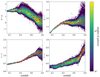 |
Fig. 1. Distribution of the selected luminous red sequence galaxies in colour space as a function of redshift (colour map). The COSMOS-G10 galaxies are shown as red stars. In each panel, the colour scale denotes the number density of luminous red galaxies in the colour-redshift space, with yellow corresponding to higher number densities and blue corresponding to lower number densities. |
Figure 1 offers an intuitive picture of how different colours contribute to determination of the redshifts of red galaxies9. At low redshifts, the g − r colour rises sharply with increasing redshift. As the 4000 Å break moves between the broadband filters, the g − r colour reaches a relative plateau while the r − i colour starts a rapid increase. At high redshifts, however, it is the i − Z colour that shows a higher sensitivity to the redshift of red galaxies. The u − g colour shows a slow and noisy decline considering that red galaxies become fainter in the u filter at higher redshifts.
3.2. Purity and completeness
For large-scale structure studies, it is important to assess the degree to which the selected red sequence galaxies are contaminated with stars. For this purpose, we define ‘purity’ as the fraction of red sequence galaxy candidates that cannot be classified as stars. Purity is meant to determine the completeness of the samples after removing the objects that can be classified as stars. We assess the purity of the sample by inspecting the distribution of the selected objects in the (r − Z, r − Ks) space. In this 2D colour space, we focus on the selected red sequence galaxies and the objects classified as high confidence star candidates in KiDS DR4, namely, the objects that have10 SG_FLAG = 0. In Fig. 2, we show the distribution of red sequence galaxies and high confidence stars in this 2D space. The left (right) panel of Fig. 2 shows this distribution for the selected objects in the dense (luminous) sample colour-coded by the estimated redshifts. The contours show the 68% and 95% of the distribution of high confidence stars in this space, respectively.
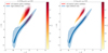 |
Fig. 2. Demonstration of the use of optical+NIR colours for the identification of likely stellar objects amongst the red sequence galaxy candidates. In each panel, the points colour-coded with redshift show the red sequence candidates in the (r − Ks)×(r − Z) space, while the blue contours show the 68% and 95% confidence regions of the distribution of stars with a high level of confidence. Left panel: at high redshifts (zred > 0.6), the considerable overlap between the distribution of red sequence candidates in the dense sample (L > 0.5 Lpivot(z)) and that of the high confidence stars becomes clear. Right panel: in the case of the red sequence candidates in the luminous sample (L > Lpivot(z)), the overlap between the two distributions is less apparent. |
As evident in the left panel of Fig. 2, there is some overlap between the distribution of the colours of galaxies in the dense sample, with zred > 0.6, and the distribution of the colours of stars with a high level of confidence. In contrast, there is a clear distinction between the colour distribution of objects in the luminous sample and that of the high-confidence stars. In both cases, there is a clear gap between the objects labelled as stars and a large majority of the selected red sequence objects. As we shall see, in the redshift range of zred > 0.6 ∼40% (∼5%) of the objects in the dense (luminous) sample are ambiguous.
The difference between the purity of the dense and the luminous samples at high redshift arises from the different size-magnitude distributions of the two samples. The objects with higher estimated redshifts tend to be fainter and smaller, making them difficult to distinguish from high-confidence stars. The objects in the dense sample, with zred > 0.6, tend to have higher apparent magnitudes and smaller sizes compared to the objects in the luminous sample. This is in line with the findings of Rozo et al. (2016), according to which the stellar contamination is higher amongst fainter red sequence objects. We can clearly see the value of the VIKING photometry in identifying the stellar contamination, resulting in an increase in the purity of our sample of LRGs.
We used Support Vector Machines (hereafter SVM, see Cortes & Vapnik 1995; Cristianini & Shawe-Taylor 2000; Schölkopf et al. 2000) to estimate a decision boundary (a line) that maximises the margin between the objects in the two classes in the 2D space. They are a class of maximum margin classifiers in which a decision boundary is chosen such that the margins between multiple classes are maximised.
It is important to note that we have made an explicit choice of feature engineering for this task: we used two features (r − Z and r − Ks) as SVM inputs to distinguish between stars and red sequence galaxies. This is motivated by our observation of the gap between the distribution of the two labels in the (r − Z, r − Ks) plane. Our motivation for using SVM is that in this 2D space, there is a clear margin between the two labels and, thus, our choice of a maximum margin classifier for this task is appropriate.
The left panel of Fig. 3 shows the predicted decision boundary (pink dashed line) separating the two red sequence objects and the high confidence stars. The selected red sequence galaxy candidates on the right hand side of the decision boundary (shown as red open circles) are likely to be stellar objects that cannot be differentiated from galaxies with morphological information only. Such objects are removed from the red sequence samples in order to maximise the purity of the sample. The red sequence sample purity (impurity) can be quantified as the fraction of red sequence candidates that lie above (below) the decision boundary shown in the left panel of Fig. 3. The right panel shows the redshift-dependence of the estimated purity of red sequence objects in the dense (luminous) sample shown in green (orange).
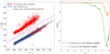 |
Fig. 3. Assessment of the purity of the red-sequence samples. At redshifts above zred > 0.4 red sequence galaxies (shown in red) and high confidence stars (shown in blue) reside in separated regions of the 2D (r − Ks)×(r − Z) colours, shown in the left panel. Shown by a pink dashed line is the predicted decision boundary between the two classes. The red sequence candidates falling below the predicted boundary are marked by open circles. These objects are flagged as likely stellar objects in the final catalogue, and thus removed from our large-scale structure analysis. Purity fraction of the dense (green dashed line) and the luminous (orange dashed line) samples as a function of redshift, in the right panel. |
Evidently, the estimated purity of galaxies in the dense sample drops significantly for zred > 0.6. On the other hand, the purity of the luminous sample remains nearly above 90% across the entire redshift range 0.1 < zred < 0.8. Excluding the contaminants from the dense sample undermines the constant comoving density of this sample for redshifts higher than 0.6.
Another important factor to take into consideration is the variable depth of the survey in the bands used in the red sequence model. In the fourth data release, the variable depth is provided by the GAaP limiting magnitudes denoted by MAG_LIM_band, where we have band = ugriZYJHKs. We inspect the distribution of the selected objects in a two dimensional (2D) space spanned by GAaP magnitude and the GAaP limiting magnitude. In particular, we aim to set the redshift reach of the samples such that the distribution of galaxies in this space is not bounded by the limiting magnitude of the survey. We carried out this investigation for the ugriZ bands.
For the griZ bands, the distribution of galaxies is not limited by the depth of the survey as long as redshift cuts of zred < 0.6 and zred < 0.8 are applied to the dense and the luminous samples, respectively. For the u-band, however, we note that even after applying the redshift cut of zred < 0.6 to the dense sample and zred < 0.8 to the luminous sample, both samples are bounded by the depth of the survey. The underlying reason for this limitation is that the red sequence galaxies become faint in the u-band at high redshifts. The possible consequences of this problem are tackled in Sect. 4, where we discuss the various survey properties that can affect the observed number density of galaxies.
3.3. Redshift distributions
For our large-scale structure studies, we constructed four redshift bins. In order to maximise the S/N of the clustering as well as that of the tangential shear signals, we made use of the dense sample as far as the purity and completeness considerations allow us (see Sect. 3.2). Hereafter, we present our work with the red sequence redshifts denoted by zred estimated in Sect. 3. We constructed three redshift bins with the dense (L > 0.5 Lpivot(z)) sample: 0.15 < zred < 0.3, 0.3 < zred < 0.45, 0.45 < zred < 0.6; along with one redshift bin with the luminous (L > Lpivot(z)) sample: 0.6 < zred < 0.8.
Table 2 summarises the characteristics of each redshift bin, including the number of objects, number of objects with secure spectroscopic redshifts, the mean redshift ⟨zred⟩, the redshift scatter, the 84th and 99.85th percentiles of the r-band magnitudes of LRGs and LRGs with spectroscopic redshift. The selected objects tend to be fainter than the objects with spectroscopic redshifts. In the last redshift bin, which encompasses the faintest objects, along with the 84th and 99.85th percentiles of the r-band GAaP magnitudes in the photometric and spectroscopic samples in the last redshift bin are [22.77, 23.58] and [21.93, 23.1], respectively. This implies that the redshift scatters quoted in Table 2 may be optimistic. The robustness of redshifts depends on the accuracy of the red sequence template, which itself is simply described by a straight line in the colour-magnitude space at each redshift (Eq. (2)). The template, estimated with brighter galaxies, is generalisable to fainter samples as long as the assumption of the red sequence template (i.e. a ridge-line in the colour-magnitude space) holds. For a sample of galaxies with spectroscopy, a comparison between the estimated red sequence redshifts and the spectroscopic redshifts is shown in Fig. 4.
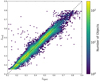 |
Fig. 4. Comparison between the estimated red sequence redshifts and spectroscopic redshifts for galaxies with spectroscopy. |
Redshift bin information.
The photometric redshift scatter, defined as the scaled median absolute deviation of the quantity (zspec − zred)/(1 + zspec), is estimated for each redshift bin. The scatter ranges between 0.012 and 0.019 with the last redshift bin zred ∈ [0.6, 0.8] having the largest scatter. Furthermore, the slight rise in scatter from the first bin to the second one can be attributed to the transition of the 4000 Å break between the broadband filters in the second redshift bin. Table 3 summarises the photometric redshift biases zred − zspec with respect to the four spectroscopic data sets. The biases are, generally, of order 10−3 with some scatter between the spectroscopic data sets. We will take this scatter into account in Sect. 5.3, where we estimate the uncertainties on the mean values of the redshift distributions of the four redshift bins.
Photo-z bias divided into four redshift bins and four spec-z data sets.
We defined the scaled redshift residuals as the difference between the spectroscopic redshifts and the red sequence redshifts, divided by the red sequence redshift uncertainties: (zspec − zred)/σz. It is useful for certain large-scale structure applications, such as galaxy clustering and galaxy-galaxy lensing, to have analytical distributions of redshift errors (scaled for redshift errors). Such analytical distributions can be utilised to estimate dN/dz needed for theoretical estimation of galaxy clustering or galaxy-galaxy lensing signals. In each redshift bin, we fit the distribution of the scaled residuals with the Normal and the Student-t parametric distributions. The probability density function of a Student-t distribution for a random variable x is given by the following form:
 (12)
(12)
 (13)
(13)
where Γ denotes the Gamma function, the shape of the distribution is controlled by the parameter ν, the parameter μ sets the mean of the distribution, and the parameter s scales the width of the distribution. For a sufficiently large value of ν, the Student t-distribution converges to a standard Normal distribution with a mean μ and a standard deviation s. In general, a smaller value of ν corresponds to a distribution with wider tails.
Figure 5 shows the distribution of the scaled redshift residuals in the second redshift bin along with the best fit Normal and Student t-distributions. The Student t-distribution provides a better description of the distribution of the redshift residuals. In particular, the tails of the distribution are better modelled by the Student-t, whereas the Normal distribution fails to capture the long tails. This implies that the individual redshift probabilities have a longer tail than what a simple Normal distribution suggests. In addition, the fat tails signal the presence of redshift outliers and such outliers are not captured by Normal distributions.
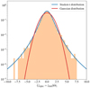 |
Fig. 5. Distribution of the quantity (zspec − zred)/σz for the second redshift bin is shown in orange, where zred and σz are per galaxy estimated quantities. In blue: best-fit Student-t distribution. In red: best-fit Gaussian distribution. The Student t-distribution provides a better description of the long tails of the redshift distributions of individual galaxies. |
In general, for all redshift bins, the Student-t distribution provides a better fit to the tails of (zspec − zred)/σz. In this work, the analytical distribution is used for estimating dN/dz. Thus, it is important to use an analytical distribution that can capture the long tails of the redshift errors in order to have an accurate theoretical model of galaxy clustering.
In each redshift bin summarised in Table 2, the distribution of the scaled redshift residuals is modelled by a Student t-distribution specified by the best-fit parameters summarised in Table 4. The redshift distributions based on this assumption will have longer tails than in the case where the individual distributions are described by a Gaussian density function. In each zred bin, the Student t-distribution provides a model for p(ztrue|zred), which is itself described by a Student t-distribution with the following shape  , mean
  , and scale
  parameters:
 (14)
(14)
 (15)
(15)
 (16)
(16)
Best-fit Student t-distribution parameters.
where the parameters (ν, μ, s) are given in Table 4.
We estimated the redshift distribution of each redshift bin by convolving dN/dzred with p(ztrue|zred), which is equivalent to summing the individual redshift probability distribution functions given by p(ztrue|zred). Figure 6 shows the redshift distributions of the four redshift bins designed for our galaxy clustering analysis. This may suggest that there is a secondary peak in the low redshift subsamples, which becomes less significant at higher redshifts. In each redshift bin, the shape of the estimated distribution is dictated by the shape of the distribution in the red sequence, zred, space as well as the shape of the redshift residual distribution (see Fig. 5). Figure 7 depicts the distribution of galaxies in zred-space. By examining Fig. 7, we see that the distribution has a dip after zred ≃ 0.2. When convolved with the redshift residual distribution (see Fig. 5), this dip results in a secondary peak in the estimated redshift distribution presented in Fig. 6.
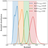 |
Fig. 6. Redshift distributions of the four redshift bins designed for studying the large-scale structure. Shaded regions mark the redshift boundaries used for defining the redshift bins. |
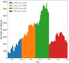 |
Fig. 7. Red sequence redshift (zred) distribution of the four redshift bins designed for studying the large-scale structure. |
4. Imaging systematics
By necessity, the data quality of large galaxy surveys such as KiDS is not homogeneous. The variable survey conditions can potentially affect the observed galaxy density and consequently can bias the cosmological inferences with these galaxy samples (Ross et al. 2012; Leistedt & Peiris 2014; Leistedt et al. 2016; Zhai et al. 2017; Elvin-Poole et al. 2018; Bautista et al. 2018; Crocce et al. 2019; Kitanidis et al. 2020; Rezaie et al. 2020; Heydenreich et al. 2020; Icaza-Lizaola et al. 2020). In this section, we first describe the imaging systematics considered in our analysis and then we discuss our mitigation strategy.
4.1. Survey properties
We consider a range of effects with on-sky variations that can impact the variations of galaxy number densities. In total, we took into account 15 survey properties that we further pixelated using HEALPIX (Górski et al. 2005). We produced the HEALPIX map of these properties with Nside = 256 (equivalent to a pixel size of 13.7 arcmin). This choice of map resolution, which was also adopted by Ross et al. (2012) and Bautista et al. (2018) in clustering measurements of LRGs, is sufficient for mitigating the systematic effects in density variations of a galaxy sample with low number density such as ours. We compute the area of each pixel at higher resolution (Nside = 4096, equivalent to 0.86 arcmin). This is the resolution at which the KiDS DR4 mask is provided. That is, the effective areas of large pixels after masking are computed using the unmasked pixels in the high resolution map with Nside = 409611.
It is important to note that the detection band in the KiDS photometry pipeline is the r-band. Therefore, many of the systematic parameters considered in our analysis are extracted from the r-band imaging data. Since we are making use of the galaxy GAaP magnitudes and magnitude errors in our red sequence pipeline, we also include the GAaP limiting magnitudes in our list of imaging systematics.
In what follows, we list the set of survey properties considered in our investigation:
Residual background counts in the THELI images: these are the background counts at the centroid positions of the objects in the THELI-processed r-band detection images. In KiDS DR4, the background count is provided as BACKGROUND. We note that the THELI processed detection images are background subtracted. The BACKGROUND parameter simply returns the value of the residual sky background at the positions of objects, therefore the background ‘counts’ could be also negative.
Detection threshold above background: this quantity is measured in units of counts. It is provided in the single-band source list as THRESHOLD.
Limiting magnitudes in 9 bands: the limiting GAaP magnitude attributes are provided in DR4 as MAG_LIM_band, where band = {u, g, r, i, Z, Y, J, H, Ks}. For each band, the limiting magnitudes are evaluated on an object-by-object basis. At the position of a given object, the limiting GAaP magnitude corresponds to the 1-σ GAaP flux error for the aperture of the source. Thus, it depends on the pixel noise in the Gaussianised image where the GAaP flux is measured, as well as the aperture size. This implies that the limiting magnitudes are indirectly dependent on the full-width-at half-maximum (FWHM) of the point spread function (PSF) in the bandpass as well as the sky background counts. Note that in our red sequence selection process, we have only used the ugriZKs bands. We note, however that since we are using the KiDS DR4 9band mask, which requires detection across all 9 bands, we also include the limiting magnitudes in the YJH bands in our imaging systematic mitigation.
PSF full width at half maximum (FWHM) in ther-band: this is the PSF FWHM in the r-band measured in units of arcseconds. The PSF FWHM is calculated using the PSF_Strehl_ratio column in the catalogue.
PSF ellipticity in ther-band: this is the KiDS PSF ellipticity in the r-band. The PSF ellipticity quantity is computed from the PSFe1, PSFe2 columns in the data.
Galactic dust extinction in ther-band: this quantity is provided as EXTINCTION_r in the nine-band catalogue of the KiDS DR4. Combination of the extinction maps by Schlegel et al. (1998) and the updated extinction coefficients from Schlafly & Finkbeiner (2011) was used to calculate the extinction coefficients in the KiDS DR4.
Star number density: we determined the stellar density from the pixelated number density map of bright stars in the second data release of Gaia (DR2, Gaia Collaboration 2018). This was done by considering the Gaia stars with the G-band magnitude between 12 and 17. This is the magnitude range in which the Gaia DR2 G-band is complete (Gaia Collaboration 2018; Arenou et al. 2018). We note that only Gaia DR2 stars that lie in the KiDS footprint are considered in the process of generating the map of stellar number densities.
The HEALPIX maps of star number densities, galactic dust extinction, detection threshold, and the residual background counts are shown in Fig. 8. The maps of the rest of the survey properties considered in this study are displayed in Figs. 12, 21, and 22 of Kuijken et al. (2019).
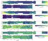 |
Fig. 8. HEALPIX maps of the density of Gaia DR2 stars with 14 < G < 17 in the KiDS DR4 footprint (first row), galactic dust extinction (second row), detection threshold above background (third row), and residual background (fourth row). All maps were generated with nside = 256. |
4.2. Impact of survey properties
We see that the survey properties considered in our investigation are correlated. Figure 9 demonstrates the mutual information between various survey properties. For instance, there is a strong anti-correlation between the residual background counts in the r-band and the stellar number density. This anti-correlation stems from the tendency of the image processing pipeline to over-estimate, and as a result, to over-subtract the sky background in the fields with higher stellar density. There is also an anti-correlation between the magnitude limit in the r-band and the PSF FWHM (middle panel of Fig. 9). This can be attributed to larger GAaP flux errors for areas of the survey with larger PSF FWHM. Conversely, there is a strong correlation between the H-band and the Ks band limiting magnitudes shown in the right panel of Fig. 9. This stems from the strong relation between the flux errors of these bands. The estimated flux errors are highly correlated in the ZY bands and HKs bands, respectively. There is also a strong, albeit with a larger scatter, correlation between the flux errors of all the NIR bands ZYJHKs. This mutual information can be attributed to the tiling strategy of the NIR bands. Another possible explanation is the anti-correlation between the limiting magnitudes and the aperture size used for estimating the GAaP flux values. A larger aperture gives rise to a lower limiting magnitude, where the effective photometric aperture is determined by the seeing in each band as well as the degree of detection in the r-band.
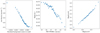 |
Fig. 9. Demonstration of the correlation between some of the survey properties. In each panel, the mean and scatter values of the survey property indicated in the label of the y-axis are shown in bins of the survey property indicated in the label of the x-axis. The anti-correlation between the residual background counts in the coadds and the stellar number density is evident (left). There is an anti-correlation between the limiting magnitude in the r-band and the PSF FWHM r-band (middle). Furthermore, there is a correlation between the NIR magnitude limits in the H and the Ks bands (right). |
Given the covariance between some of the survey properties, we inspect the variation of the observed galaxy number densities and the survey properties in the linear basis, in which the covariance matrix between the parameters is diagonal. The basis vectors of this space are the eigen-vectors of the covariance matrix of survey properties12. In this new basis, we can assess the variations between the observed galaxy number density and the different basis vectors independently.
In particular, we inspect the variation of galaxy over-densities δgal = ngal/⟨ngal⟩, where ngal is galaxy number density in units of arcmin−2. As pointed out in Sect. 4.1, the pixel areas in the HEALPIX maps with Nside = 256 are calculated using a higher resolution HEALPIX map of KiDS DR4 mask with resolution of Nside = 4096. In each pixel in the healpix map, with Nside = 256, ngal is calculated by dividing the number of galaxies in that pixel by the area of that pixel. The quantity ⟨ngal⟩ is calculated by simply taking the mean of ngal for a given galaxy sample. Any deviation of this quantity from unity as a function of an imaging systematic indicates a non-vanishing impact of that systematic13. We denote the list of all pixelated survey property parameters by  , where the subscript i denotes the position of the pixel i on the sky. Furthermore, we transformed the set of vectors
  so that the mean and the variance across each of the 15 dimensions are zero and one, respectively. Afterwards, we transform this 15-dimensional linear basis to a new orthogonal basis, in which the covariance matrix of the survey property vectors is diagonal. In this new basis, we represent the list of survey property parameters by
  where at each pixel we have:
![Mathematical equation: $$ \begin{aligned} {\boldsymbol{S}}_{\perp } = [S_{\perp }^{(1)}, S_{\perp }^{(2)}, \ldots , S_{\perp }^{(15)}], \end{aligned} $$](/articles/aa/full_html/2023/07/aa39293-20/aa39293-20-eq43.gif) (17)
(17)
where  is the jth systematic vector in the new basis. The relation between the survey properties and the orthogonal features is illustrated in Fig. 10. It is clear that the first orthogonal feature is dominated by the near-IR limiting magnitudes. The second feature
  is related, with negative signs, to the residual background counts, detection threshold, and the r-band limiting magnitude and related, with positive signs, to the star density and the dust extinction.
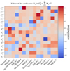 |
Fig. 10. Relation between the set of orthogonal survey features |


For the third redshift bin14 (zred ∈ [0.45, 0.6]), the variation of the observed number density versus the survey property parameters, S⊥, is shown by the red error-bars in Fig. 11, where in each panel, the red error-bars show the mean and scatter values of the galaxy over-densities in bins of the survey property indicated by the x-axis. We have only shown the four most significant variations quantified by the null chi-squared  , with higher values of
  corresponding to higher deviations of galaxy densities in relation to the survey properties. For instance, the most significant systematic mode present in density variation of galaxies in the third redshift bin is due to the feature
  , which itself is dominated by the magnitude limit in the u-band. The strong
  systematic mode in the third redshift bin (the highest redshift bin constructed from the dense sample) is due to the fact that the u-band magnitude distribution of the high redshift galaxies in our sample is limited by the depth of the survey in this band.
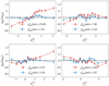 |
Fig. 11. Variation of the galaxy overdensity versus the orthogonal survey property parameters {S⊥} in the third redshift bin zred ∈ [0.45, 0.6], with (in blue) and without (in red) the photometric weights included. The deviation of the galaxy over density from unity is quantified by |


It is clear that the galaxy density in our sample correlates with survey properties. Therefore, we mitigated the impact of systematics by introducing a set of photometric weights. This approach has been widely utilised in galaxy clustering analyses: the clustering of LRGs in SDSS BOSS (Ross et al. 2012, 2017), galaxy clustering in the Dark Energy Survey (Elvin-Poole et al. 2018; Crocce et al. 2019), DESI legacy survey (Kitanidis et al. 2020), and finally clustering of LRGs in SDSS-eBOSS (Bautista et al. 2018; Icaza-Lizaola et al. 2020).
Following the work of Bautista et al. (2018), we computed the photometric weights by assuming a relation between the pixelated observed galaxy overdensities and δgal = Ngal/⟨Ngal⟩ and the set of pixelated systematic parameters. In Bautista et al. (2018), this relation is assumed to be linear, namely, δgal = Ws + b + noise. Additionally, we consider two modifications. First, we introduced a set of second-order polynomial features from the original feature space {s}. The second-order features consist of all possible combinations of {sisj} as well as single features {si}. These polynomial features are then mapped to the observed galaxy densities via a linear relation. By accounting for the second-order polynomial features, we have W, a 136-dimensional vector to be estimated from the regression. Furthermore, we introduce an L2 regularisation to this regression problem which is implemented by adding a regularisation term  to the least square cost function. The added advantage of this regularisation term is that it tends to keep the W parameters small thereby avoiding overfitting.
In practice, we chose the regularisation hyper-parameter λ by a k-fold cross-validation search in which we explored a wide range of λ values from 10−4 to 105. We note that in all the redshift bins, our cross-validation optimisation procedure prefers a heavy regularisation in which a very large value of λ ∈ [103 − 105] is favoured. The advantage of this approach over that of Ross et al. (2017) is that we do not assume that there is no correlation between the systematic parameters.
The prediction of this model, once it is applied to the pixelated systematic maps, provides a set of photometric weights that remove the systematically induced variations in the galaxy number density. The photometric weight of a single galaxy is obtained by taking the inverse of the output of the regression model at the healpix pixel containing that galaxy. Figure 11 demonstrates how the photometric weights derived from our framework can help reduce the systematic trends seen in the observed galaxy number densities. In Fig. 11, the density-correlations are displayed after taking into account the photometric weights (shown in blue) and without the photometric weights (shown in red). We note that the reduced χ2 improves significantly once the photometric weights are taken into consideration.
We also investigated the two-point cross-correlations of the galaxy number density and the orthogonal systematic parameters  as a function of angular separation in our galaxy sample. We find that the cross correlations, before and after including the photometric weights, are consistent with zero (albeit with slight improvements once the photometric weights are taken into account).
Alternatively, one can use self organising maps (SOM, Kohonen 1997) for learning the systematic galaxy density modes due the variable survey properties and then generating a set of ‘organised randoms’ mimicking the galaxy depletion pattern across the survey footprint. We have also tested this method and we found that this method works best in correcting the systematic depletion in a galaxy sample with a higher number density than in our study. This approach is being pursued by Johnston et al. (2021) to mitigate the systematic biases in clustering of galaxies in the KiDS DR4 bright sample (Bilicki et al. 2021).
We did not explore the effect of various observing conditions on the distribution of derived physical properties of the galaxies. Such effects can in principle generate systematic on-sky variations of the estimated host halo mass of galaxies in our sample, which can subsequently complicate the cosmological analysis. This problem is exacerbated in a galaxy survey covering a larger area, due to significant reduction in statistical uncertainty, and can only be taken into account through a careful forward model approach, which is beyond the scope of this paper.
5. Galaxy clustering
5.1. Theory
Assuming a local deterministic linear galaxy bias, the galaxy overdensity, δg, is related to the matter overdensity, δm, through a linear relation: δg = bgδm, where the parameter bg is the linear bias parameter. Such an assumption is expected to hold on sufficiently large scales (e.g. Kravtsov & Klypin 1999; Marian et al. 2015), whereas on small scales, the nonlinear structure formation is best described by the more sophisticated halo model (e.g. Berlind & Weinberg 2002; Cooray & Sheth 2002; Zehavi et al. 2011; Hand et al. 2017; Vakili & Hahn 2019).
Given a nonlinear matter power-spectrum, PNL(k, z), and a galaxy population with linear bias of bg and redshift distribution ng(z), we can predict the angular two-point correlation function wg(θ). Under the assumption of flat universe, and the Limber- and flat-sky approximations (Limber 1961; Loverde & Afshordi 2008; Kilbinger et al. 2017; Kitching et al. 2017), the angular clustering wg(θ) is given by:
![Mathematical equation: $$ \begin{aligned} { w}_{\rm g}(\theta ) =&b_{\rm g}^2 \int _{0}^{\infty } \frac{l\mathrm{d}l}{2\pi }J_{0}(l\theta )\nonumber \\&\times \int _{0}^{\chi _{\rm H}} \mathrm{d}\chi _{\rm c} \left[\frac{n_{\rm g}(z)\frac{\mathrm{d}z}{\mathrm{d}\chi _{\rm c}}}{\chi _{\rm c}}\right]^{2}P_{\rm NL}\left(\frac{l+1/2}{\chi _{\rm c}}; z\right), \end{aligned} $$](/articles/aa/full_html/2023/07/aa39293-20/aa39293-20-eq59.gif) (18)
(18)
where χc is the comoving distance to redshift, z, χH the Hubble distance, and J0 the 0th order Bessel function of the first kind. The nonlinear power spectrum can be calculated using different recipes such as the halo model (e.g. Takahashi et al. 2012; Mead et al. 2015; Smith & Angulo 2019), or emulation (e.g. Heitmann et al. 2014). Hereafter, we use the Core Cosmology Library (CCL, Chisari et al. 2019a,b) to compute the theoretical predictions of angular clustering. We used the Takahashi et al. (2012) model as it is capable of predicting the matter clustering in the linear and quasi-linear regimes (i.e. χc > 8 Mpc h−1) considered in this study.
We calculated the theoretical prediction (Eq. (18)) for all four redshift bins in our galaxy sample with their corresponding linear bias parameters  and redshift distributions
  . We used the redshift distributions computed in Sect. 3.3.
Assuming a fixed cosmology, we aim to estimate the linear bias parameters  by fitting the theoretical prediction (18) to the angular clustering of our LRG samples. It is worth noting that one major source of systematic error in this theoretical prediction is the uncertainty on the mean of the redshift distributions
  . In order to mitigate its impact, we assume that the estimated redshift distribution at each redshift bin
  is effectively given by shifting the underlying unbiased redshift distribution
  , where the parameter δz(i) is the uncertainty on the mean of the redshift distribution of ith redshift bin. In Sect. 5.3, we discuss how the uncertainty over the mean of the redshift distribution can be estimated. When reporting the constraints on the galaxy bias parameters, we marginalise over the redshift uncertainties.
5.2. Clustering measurements
The galaxy two-point correlation function is the excess probability (compared to a random one) of finding a pair of galaxies within a given angular or physical separation. Given that we do not know the exact redshifts of the galaxies, we focus on computing the angular correlation function which can be obtained by performing pair-counts in angular bins perpendicular to the line of sight. We measure the angular clustering using the Landy–Szalay estimator (Landy & Szalay 1993):
 (19)
(19)
where DD denotes the number of galaxy pairs within an angular separation bin centred at θ, DR denotes the number of galaxy-random pairs, and RR denotes the number of random pairs. The random points are uniformly distributed within the survey footprint.
The construction of random points is as follows. First, we generate a large number of randoms uniformly distributed over the sphere. We use a healpix binary mask with Nside = 4096 to limit the random points to the survey footprint. This Healpix mask is constructed such that it is consistent with the mask described in Sect. 2.115. At the end, we choose a random subsample of 2 million points from the random points in the survey footprint. The size of the random sample is therefore ∼16 times larger than the size of the galaxy sample in the third tomographic bin.
As discussed in Sect. 4, in each redshift bin a photometric weight is assigned to each galaxy depending on its position on the sky. These weights are derived such that the on-sky variations of galaxy overdensity due to survey properties are mitigated. We compute two sets of angular clustering measurements, one with the photometric weights, and another without. In the presence of weights, the DD and DR pair count calculations are modified in the following way:
 (20)
(20)
 (21)
(21)
where Θij(θ) = 1(0) when a galaxy-galaxy, or a galaxy-random pair in the case of DR, (indexed by i, j) are (are not) within the angular bin centred on θ, and ωi is the photometric weight associated with the ith galaxy.
The angular clustering measurements of LRGs in four redshift bins are displayed in Fig. 12, with the first three bins encompassing the galaxies in the dense (L > 0.5 Lpivot(z)) sample and the last bin (0.6 < z < 0.8) encompassing the galaxies in the luminous (L > Lpivot(z)) sample. The clustering signal estimated with (without) the photometric weights is shown in blue (orange). The correlation functions are measured in 15 logarithmically spaced bins in the range 10 ≤ θ ≤ 100 arcmin. Although the lowest angular limit of 10 arcmin is lower than the systematic map resolution of 13 arcmin, the scale cuts (see Sect. 5.3.2) that will be applied to our clustering data vectors will be larger than both of these angular scales.
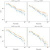 |
Fig. 12. Clustering measurements for the four redshift bins. In each panel, the blue (orange) data points correspond to the correlation functions computed with (without) the photometric weights designed to remove survey-related systematic density variations. |
Based on Fig. 12, it appears that without the photometric weights, the amplitude of the measured clustering is higher. This is expected if the number of detected galaxies is affected by variations in depth (e.g. low limiting magnitude, high seeing) in certain regions. As a result, the galaxy sample may appear more clustered on those scales. Therefore, if not accounted for, the survey systematics can lead to a higher clustering signal.
We estimated the measurement uncertainties using the jackknife resampling method (Norberg et al. 2009; Friedrich et al. 2016; Singh et al. 2017; Shirasaki et al. 2017). In this method, the KiDS survey footprint is first divided into NJK = 100 contiguous jackknife subsamples of approximately equal area16. For each subsample k ∈ {1, …, NJK}, the clustering data vector  is measured by dropping the kth subsample and estimating the clustering signal from the rest of the survey area. We note that the vector
  contains the correlation function measured in all the 15 angular bins considered in this study. The jackknife estimator of the covariance matrix is then given by:
 (22)
(22)
where  is the mean of all
  vectors.
Since the covariance matrix is estimated from the jackknife method with a finite number of jackknife subsamples, our estimate of the covariance matrix and its inverse are noisy. The unbiased estimate of the inverse covariance matrix is related to the inverse of the estimated jackknife covariance matrix  with the Anderson-Hartlap-Kaufman (Kaufman 1967; Hartlap et al. 2007) debiasing factor:
 (23)
(23)
where NJK is the number of jackknife subsamples and Nd is the number of bins, in the clustering measurements, that enter the likelihood function evaluation. Since we removed the nonlinear scales from our likelihood analysis, only the data points that pass the cuts are those that determine the number of data points Nd appearing in Eq. (23).
5.3. Inference setup
5.3.1. Parameters
In order to fit the theoretical model of angular clustering to the data, we needed to clarify our choices of parameters. Assuming a fixed cosmology, we estimated the linear galaxy bias (using Eq. (18)) of the red galaxies in the redshift bins. We estimated the bias parameters by marginalising over the photometric redshift uncertainty parameters. Furthermore, we chose a flat LCDM model assuming Ωm = 0.25, ΩΛ = 0.75, Ωb = 0.044, σ8 = 0.8, ns = 0.95, h = 0.7, which is the input cosmology of the MICE suite of cosmological simulations (Fosalba et al. 2015). We picked this set of cosmological parameters for the purposes of carrying out an internal comparison (Fortuna et al. 2021). However, given that the amplitude of galaxy clustering depends on the amplitude of the power spectrum, growth factor, and galaxy bias, we expect our bias constraints in this work to depend on the assumed cosmology.
We adopted the following priors on the model parameters. For the galaxy bias parameters, we assume a uniform prior with a lower bound of 1 and an upper bound of 3. For the prior distribution of the photo-z shift parameters  , we assumed a Gaussian distribution with zero mean and a dispersion, which we estimated in the following way. We first assume that there are two major contributions to the uncertainty of the mean of the redshift distributions. The first contribution is the spatial sample variance that we compute using the jackknife resampling method. The second contribution is estimated by computing the covariance between the photo-z biases with respect to the four spectroscopic redshift surveys considered in this study (see Table 3). Combining these two sources of uncertainty provides us with an estimate of the prior distribution over the photo-z shift parameters:
 (24)
(24)
where σδzi is 2.4 × 10⁻³, 3.2 × 10⁻³, 2.3 × 10⁻³, and 4.6 × 10⁻³ for the first, second, third, and fourth redshift bins, respectively.
5.3.2. Scale cuts
The theoretical model summarised in Eq. (18) fails to capture the full complexity of the galaxy-matter connection on small scales as it relies only on a simple linear deterministic treatment of galaxy bias. Therefore, we decided to apply a conservative cut on the comoving scales considered in our theoretical modelling of the clustering signal. In particular, we adopt a cut at a comoving scale of 8 Mpc h−1 which translates to a minimum angular scale (hereafter, denoted as θmin) of 39.8 arcmin for the first bin, 25.9 arcmin for the second bin, 19.3 arcmin for the third bin, and, finally, 15.2 arcmin for the last redshift bin. The comoving distance is converted to angular scales assuming the flat ΛCDM cosmology discussed above. Furthermore, the parameter θmin in each redshift bin is calculated from dividing the minimum comoving scale of 8 Mpc h−1 by the comoving distance at the mean redshift of the redshift bin under consideration.
5.3.3. Likelihood and posterior sampling
With the theoretical model, the measurements, and the covariance matrix at hand, now we are ready to constrain the linear galaxy bias and photo-z distribution shift parameters for each redshift bin:  . We performed the inference for each redshift bin separately. Therefore, for each redshift bin, we simultaneously constrained two parameters: the linear galaxy bias and photo-z distribution shift.
We assumed that the likelihood is a multivariate Gaussian distribution with the mean given by the theoretical prediction (Eq. (18)) and with the inverse covariance matrix (Eq. (23)). The model parameters are constrained by MCMC sampling from the posterior probability distribution p(θ|d)∝p(d|θ)p(θ) using the emcee implementation (Foreman-Mackey et al. 2013) of the affine-invariant ensemble Markov chain Monte Carlo sampling method of Goodman & Weare (2010)17.
5.4. Constraints
Figure 13 presents measurement of the angular correlation function (data points with error bars) together with the 68% and 95% posterior predictions of wθ for all the four redshift bins. Given the uncertainties, the model predictions are consistent with the measurements. The 1σ and 2σ levels of the 2D posterior surfaces in the (bg, δz) parameter space as well as the marginalised distributions over the individual parameters are displayed in Fig. 14. The correlation between the inferred bias parameter and the photo-z shift parameter appears to be very small. The Spearman correlation18 between the two parameters is 0.02, 0.06, 0.06, and 0.06 for the four bins in increasing redshift order.
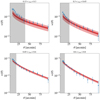 |
Fig. 13. Comparison between the posterior predictions (red shaded) of clustering and the clustering measurements (blue points with error bars) in the four redshift bins. The dark and light shaded regions mark the 68% and the 95% confidence intervals. The error bars are derived from the diagonal elements of the covariance matrix of the observations. |
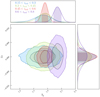 |
Fig. 14. Joint constraints on the linear galaxy bias and photo-z shift parameters shown for the redshift bins constructed with the dense sample (blue contours) and the last redshift bin which is constructed from the luminous sample (red contour). |
Furthermore, we use the scipy library to optimise the posterior probability to find the best-fit parameters and in order to estimate the reduced χ2 (hereafter  ) corresponding to the best-fit parameters for each redshift bin. The obtained
  are 0.28, 2.80, 2.01, and 0.65 for the first to the last redshift bin, respectively.
The marginalised distributions are summarised in Table 5. We note that the constraints on the photo-z shift parameters are consistent with zero and largely consistent with the adopted priors over these parameters. Furthermore, we find consistency, given the uncertainties, between the constraints on the galaxy bias parameters of the first three bins. We note that the first three bins are constructed from the dense galaxy sample, which has an approximately constant comoving density. On the other hand, our constraint on the bias parameter of the last bin is higher than those of the first three bins. This is expected as the last bin is constructed from the luminous sample, which consists of brighter galaxies residing in more massive halos.
Summary of the parameter constraints.
In the default setup for studying the large-scale structure, we have relied on four redshift bins, three of which are constructed from the dense sample with bins defined by the redshift edges of [0.15, 0.3, 0.45, 0.6], and one last bin constructed from the luminous sample within the [0.6, 0.8] redshift interval. In order to assess the redshift-dependence of the estimated bias parameters, we defined two additional redshift bins for the galaxies in the luminous sample with the redshift edges of [0.2, 0.4, 0.6]19. Following the steps discussed above for our fiducial large-scale structure analysis, we performed a photometric weight assignment, correlation function measurement of these two redshift bins in the luminous sample.
The redshift dependence of the bias is shown in Fig. 15, where the estimated bias parameters of the luminous (dense) sample are shown in red (blue). The boxes mark the 68% as well as the 95% confidence intervals in the marginalised bias distributions. We note that within each sample, the bias constraints do not appear to have any strong redshift evolution. We also note that for the dense sample, our linear bias constraints are consistent with the findings of Brown et al. (2008), where they studied the clustering of photometrically selected red galaxies in different ranges of redshift and comoving density.
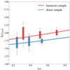 |
Fig. 15. Redshift dependence of the estimated linear galaxy bias shown for the dense sample (blue) and the luminous sample (red). The boxes mark the 68% and the 95% confidence intervals of the marginalised distribution over bias parameters. The solid (dashed) lines show the predictions of the passive evolution model of Fry (1996) given the bias constraints in the three redshift bins (in the last redshift bin) for each galaxy sample. |
We compare our findings with the passive evolution model of galaxy bias (see Fry 1996; Tegmark & Peebles 1998) according to which, the evolution of the linear bias follows:
 (25)
(25)
where D(z) is the linear growth factor normalised to unity at z = 0, and b0 the linear bias at z = 0. The passive evolution model has been tested against the amplitude of the clustering of LRGs in Tojeiro et al. (2012), Guo et al. (2013). In particular, this latter study investigated the evolution of the large-scale bias of red galaxies for various ranges of constant comoving density, and absolute magnitude, as well as colour. Following the approach of Guo et al. (2013), we fit the passive evolution model to our estimated biases as a function of redshift in two samples.
We begin by describing the bias evolution of the luminous sample. By fitting the passive evolution model of Fry (1996) to the bias constraints in the luminous sample, we find that this model provides a good picture of the evolution of galaxy bias (red solid line in Fig. 15). When constraining the passive evolution model with the bias estimate of the highest redshift bin (0.6 < zred < 0.8), we find that the expected bias parameters for the first and the second bins are consistent with the estimated parameters within 1σ levels (red dashed line in Fig. 15).
Turning our attention to the dense sample, we find that the passive evolution model still provides a consistent picture of bias evolution (blue solid line in Fig. 15). Once we condition the passive evolution model on the bias constraint of the highest redshift bin (0.45 < zred < 0.6), we find that the expected bias values for the first and the second redshift bins are in perfect agreement with the inferred bias parameters (blue dashed line in Fig. 15). Overall, we find that the redshift evolution of the bias of our LRG samples is consistent with the passive evolution model. Although this consistency can be attributed to the large error bars on the estimated biases of the two samples.
5.5. Comparison of bias constraints with other studies
Zhai et al. (2017) studied the clustering of LRGs in a combined BOSS+eBOSS sample at z ∼ 0.7. The estimated bias of that sample is 2.3 ± 0.03, which is higher than the estimated bias of our sample of LRGs in the highest redshift. The number density of that sample, however, is approximately 1.4 × 10⁻⁴, which is lower than that of our sample.
Elvin-Poole et al. (2018) analysed the clustering of redmagic galaxies in DES Year-1 data. The first three redshift bins in Elvin-Poole et al. (2018) are constructed in a similar manner with luminosity L/Lpivot(z) > 0.5. However, this luminosity ratio and the magnitude in red sequence template use the z-band while in our work these quantities use the KiDS r-band. The fourth redshift bin in that study has a ratio threshold of L/Lpivot(z) > 1 with the upper bound of the redshift bin being 0.75 instead of 0.8. The estimated linear bias parameters in the first to fourth redshift bins are 1.4 ± 0.07, 1.6 ± 0.05, 1.6 ± 0.04, 1.98 ± 0.07, which compared to the estimated bias parameters in our work (see Table 5), are slightly lower in the first three bins and consistent in the fourth bin.
Zhou et al. (2021) analysed the clustering of a photometrically-selected sample of LRGs selected in the Legacy Survey imaging data. This sample was selected so that it would emulate the sample of LRGs from the Dark Energy Spectroscopic Instrument survey (DESI Collaboration 2016). The range of photometric redshifts of these galaxies is 0.41 < z < 0.93 with the number densities ranging from ∼2.1 × 10⁻⁴ (h−1 Mpc)−3 to ∼6.3 × 10⁻⁴ (h−1 Mpc)−3. In that study, in the two redshift bins of 0.61 < z < 0.72 and 0.75 < z < 0.83 the number densities are ∼6.1 × 10⁻⁴ (h−1 Mpc)−3 and ∼4.4 × 10⁻⁴ (h−1 Mpc)−3, respectively. The estimated bias parameters of these two samples are 2.07 ± 0.03 and 2.24 ± 0.8 – values that are both higher than the estimated bias of 2.01 ± 0.08 of galaxies in our fourth redshift bin. The LRG selection process of Zhou et al. (2021), however, is different than that of ours in that they use simple color-magnitude cuts and do not rely on a red sequence template-based sample selection.
6. Summary
In this work, we introduce the selection and clustering measurements of red sequence galaxies in the fourth data release of the Kilo-Degree Survey. The data-driven colour-redshift relation of these galaxies allows us to obtain precise and accurate estimates of their photometric redshifts. We constructed two samples, a bright one and a dense one, each with approximately constant comoving density.
We find that the near-infrared magnitudes derived from the VIKING imaging of the selected galaxies allow us to assess the purity of the sample. This purity assessment was done by comparing the colour distribution of the red sequence candidates and that of high-confidence stars in the fourth data release. The outcome of this procedure is the removal of ∼40% of the candidates in the dense sample with zred > 0.6 and ∼5% of the candidates in the luminous sample in the same redshift range.
After taking into account the purity and completeness of the samples, we constructed four redshift bins for our large-scale structure analysis, with the first three bins based on the dense sample and the last bin based on the bright sample. In order to estimate the redshift distributions as well as the uncertainty over the mean redshift of the distributions, we relied on four spectroscopic redshift surveys. Of these redshift surveys, three have an overlap with the fourth data release, while GAMA-G10 only covers one of the KiDS calibration fields in the COSMOS region. In each redshift bin, the individual redshift distributions of galaxies are well described by a Student t-distribution, parameters of which are estimated with the overlapping spectroscopic data sets.
In order to account for the impact of the data quality, we extended the works of Bautista et al. (2018) and Icaza-Lizaola et al. (2020) to allow for a more flexible relation between the systematic-induced variations of observed galaxy densities and survey properties, while making use of heavy regularisation to avoid overfitting. In comparison to Ross et al. (2012), Crocce et al. (2019), our adopted framework for removing the impact of survey properties does not make any assumption regarding the lack of correlation between the survey properties. Having validated our method for removing the effect of imaging systematics on the observed density variations, we applied the derived photometric weights to the measurement of the red sequence galaxy clustering.
We find that the estimated bias parameters of the galaxies in the L > 0.5 Lpivot(z) sample are lower than those of L > Lpivot(z) sample, which is consistent with the expectation that brighter galaxies reside in higher mass halos. The constraints on the photo-z shift parameters are consistent with zero and largely consistent with the adopted priors over these parameters. By comparing the redshift evolution of our bias constraints with the passive evolution model, we find that the bias evolution of galaxies in both dense and luminous samples is consistent with the expectations inherent in the model.
KiDS-1000 and KiDS DR4 refer to the same dataset.
In the near-infrared photometry of the cosmos region, the CFHTLS Z-band is used.
The redshifts of SDSS DR13 and GAMA galaxies are reported in the heliocentric frame while the redshifts of the 2dFLenS galaxies are reported in the CMB rest frame.
Calculated assuming a ΛCDM model with Planck (Planck Collaboration XIII 2016) best-fit parameters. We find that the choice of cosmology has no impact on the estimated red sequence redshifts and sample selection.
We refer the readers to Appendix C for a description of morphological and physical properties of these samples.
Note that in this intuitive description we have neglected the magnitude dependence of the red sequence template which plays an additional constraining role in determining the redshifts.
The SG_FLAG parameter makes use of the size-peakiness relation of objects in order to determine whether they can be classified as star or not.
We are interested in measuring the two-point correlation function on large scales. Therefore, calculating the effective areas of pixels in the low resolution map with Nside = 256, with the higher resolution mask map with Nside = 4096 is sufficient for the purpose of this study.
Prior to diagonalisation of the covariance matrix of survey properties, we apply a log-transformation to the parameters whose distributions have long tails.
Note that alternatively, one can reformulate this by looking at the deviations of Ngal/Nrandom (modulo some normalisation) from unity, where Nrandom is the number density of a set of uniformly distributed random points across the survey footprint (e.g. Bautista et al. 2018; Icaza-Lizaola et al. 2020).
For brevity we only show the survey property-density trends in the third bin. The trends in the rest of the redshift bins and the corrections are similar.
It is implicitly assumed that each pixel in the healpix map with Nside = 4096 is complete.
The segmentation of KiDS DR4 footprint into NJK is done with the K-means algorithm. We made use of an implementation of this algorithm designed to handle RA and Dec coordinates on the sky (https://github.com/esheldon/kmeans_radec).
We run emcee with 20 walkers and 4000 iterations. The auto-correlation method of emcee suggests that all our chains converge after a few hundred iterations. We drop the first 1000 iterations and keep the last 3000 for our final constraints.
The Spearman correlation coefficient provides an estimate of the monotonicity in the relation between two parameters without assuming that the distribution of the parameters is Normal (Zwillinger & Kokoska 1999).
These two redshift bins constructed from the luminous sample are not part of our fiducial clustering analysis. They are only introduced in this section to assess the redshift dependence of the galaxy bias in the luminous sample.
We also experimented with different choice of slicing the redshift but we did not see any major impact on the selection of seed galaxies. Our choice of wider redshift slice of 0.04 for the highest redshift range 0.7 < z < 0.82 is due to relative sparsity of the spectroscopic galaxy sample at higher redshifts.
We have tried different choices of spacing for these parameters and after optimising the objective function (Eq. B.1) we have found that the parameter with the most (least) significant variation is a(z)(Cint(z)).
Acknowledgments
M.V., H.Ho. and M.C.F. acknowledge support from Vici grant 639.043.512 from the Netherlands Organization of Scientific Research (NWO). M. Bilicki is supported by the Polish National Science Center through grants no. 2020/38/E/ST9/00395, 2018/30/E/ST9/00698, 2018/31/G/ST9/03388 and 2020/39/B/ST9/03494, and by the Polish Ministry of Science and Higher Education through grant DIR/WK/2018/12. H.J. acknowledges support from a UK Science and Technology Facilities Council (STFC) Studentship. A.H.W. is supported by an European Research Council Consolidator Grant (No. 770935). M.A. acknowledges support from the European Research Council under grant number 647112. B.G. acknowledges support from the European Research Council under grant number 647112 and from the Royal Society through an Enhancement Award (RGF/EA/181006). C.H. acknowledges support from the European Research Council under grant number 647112, and support from the Max Planck Society and the Alexander von Humboldt Foundation in the framework of the Max Planck-Humboldt Research Award endowed by the Federal Ministry of Education and Research. H. Hildebrandt is supported by a Heisenberg grant of the Deutsche Forschungsgemeinschaft (Hi 1495/5-1) as well as an ERC Consolidator Grant (No. 770935). S.J. acknowledges support from the Beecroft Trust and ERC 693024. GAMA is a joint European-Australasian project based around a spectroscopic campaign using the Anglo Australian Telescope. The GAMA input catalogue is based on data taken from the Sloan Digital Sky Survey and the UKIRT Infrared Deep Sky Survey. Complementary imaging of the GAMA regions is being obtained by a number of independent survey programs including GALEX MIS, VST KiDS, VISTA VIKING, WISE, Herschel-ATLAS, GMRT and ASKAP providing UV to radio coverage. GAMA is funded by the STFC (UK), the ARC (Australia), the AAO, and the participating institutions. The GAMA website is http://www.gama-survey.org. Funding for SDSS-III was provided by the Alfred P. Sloan Foundation, the Participating Institutions, the National Science Foundation, and the US Department of Energy Office of Science. The SDSS-III website is http://www.sdss3.org/. SDSS-III is managed by the Astrophysical Research Consortium for the Participating Institutions of the SDSS-III Collaboration including the University of Arizona, the Brazilian Participation Group, Brookhaven National Laboratory, Carnegie Mellon University, University of Florida, the French Participation Group, the German Participation Group, Harvard University, the Instituto de Astrofisica de Canarias, the Michigan State/NotreDame/JINA Participation Group, Johns Hopkins University, Lawrence Berkeley National Laboratory, Max Planck Institute for Astrophysics, Max Planck Institute for Extraterrestrial Physics, New Mexico State University, New York University, Ohio State University, Pennsylvania State University, University of Portsmouth, Princeton University, the Spanish Participation Group, University of Tokyo, University of Utah, Vanderbilt University, University of Virginia, University of Washington, and Yale University. This work has made use of python (http://www.python.org/), including the packages numpy (http://www.numpy.org/), scipy (http://www.scipy.org/), pandas (https://pandas.pydata.org/), and scikit-learn (https://scikit-learn.org/). Plots have been produced with matplotlib (https://matplotlib.org/) and seaborn (https://seaborn.pydata.org/). We have used the ChainConsumer package (Hinton 2016) to generate Fig. 14 of the paper. This work has made use of CosmoHub (https://cosmohub.pic.es/). CosmoHub (cosmohub.pic.es) has been developed by the Port d’Informació Científica (PIC), maintained through a collaboration of the Institut de Fisica d’Altes Energies (IFAE) and the Centro de Investigaciones Energeticas, Medioambientales y Tecnologicas (CIEMAT) and the Institute of Space Sciences (CSIC & IEEC), and was partially funded by the “Plan Estatal de Investigacion Cientifica y Tecnica y de Innovacion” program of the Spanish government. Author contributions: All authors contributed to the development and writing of this paper. The authorship list is given in three groups: the lead authors (MV,HHo, MB, MCF) followed by two alphabetical groups. The first alphabetical group includes those who are key contributors to both the scientific analysis and the data products. The second group covers those who have either made a significant contribution to the data products, or to the scientific analysis.
References
- Abbott, T. M. C., Abdalla, F. B., Alarcon, A., et al. 2018, Phys. Rev. D, 98, 043526 [NASA ADS] [CrossRef] [Google Scholar]
- Abbott, T. M. C., Aguena, M., Alarcon, A., et al. 2022, Phys. Rev. D, 105, 023520 [CrossRef] [Google Scholar]
- Alam, S., Ata, M., Bailey, S., et al. 2017, MNRAS, 470, 2617 [Google Scholar]
- Albareti, F. D., Allende Prieto, C., Almeida, A., et al. 2017, ApJS, 233, 25 [Google Scholar]
- Arenou, F., Luri, X., Babusiaux, C., et al. 2018, A&A, 616, A17 [NASA ADS] [CrossRef] [EDP Sciences] [Google Scholar]
- Arnouts, S., Cristiani, S., Moscardini, L., et al. 1999, MNRAS, 310, 540 [Google Scholar]
- Asgari, M., Lin, C.-A., Joachimi, B., et al. 2021, A&A, 645, A104 [NASA ADS] [CrossRef] [EDP Sciences] [Google Scholar]
- Bautista, J. E., Vargas-Magaña, M., Dawson, K. S., et al. 2018, ApJ, 863, 110 [NASA ADS] [CrossRef] [Google Scholar]
- Berlind, A. A., & Weinberg, D. H. 2002, ApJ, 575, 587 [Google Scholar]
- Bertin, E., & Arnouts, S. 1996, A&AS, 117, 393 [NASA ADS] [CrossRef] [EDP Sciences] [Google Scholar]
- Bilicki, M., Dvornik, A., Hoekstra, H., et al. 2021, A&A, 653, A82 [NASA ADS] [CrossRef] [EDP Sciences] [Google Scholar]
- Blake, C., Amon, A., Childress, M., et al. 2016, MNRAS, 462, 4240 [NASA ADS] [CrossRef] [Google Scholar]
- Bower, R. G., Lucey, J. R., & Ellis, R. S. 1992, MNRAS, 254, 601 [NASA ADS] [CrossRef] [Google Scholar]
- Brown, M. J., Zheng, Z., White, M., et al. 2008, ApJ, 682, 937 [NASA ADS] [CrossRef] [Google Scholar]
- Bruzual, G., & Charlot, S. 2003, MNRAS, 344, 1000 [NASA ADS] [CrossRef] [Google Scholar]
- Cacciato, M., van den Bosch, F. C., More, S., Mo, H., & Yang, X. 2013, MNRAS, 430, 767 [Google Scholar]
- Capaccioli, M., Schipani, P., de Paris, G., et al. 2012, Science from the Next Generation Imaging and Spectroscopic Surveys, 1 [Google Scholar]
- Chabrier, G. 2003, PASP, 115, 763 [Google Scholar]
- Chang, C., Baxter, E., Jain, B., et al. 2018, ApJ, 864, 83 [NASA ADS] [CrossRef] [Google Scholar]
- Chisari, N. E., Alonso, D., Krause, E., et al. 2019a, ApJS, 242, 2 [Google Scholar]
- Chisari, N. E., Alonso, D., Krause, E., et al. 2019b, Astrophysics Source Code Library [record ascl:1901.003] [Google Scholar]
- Contigiani, O., Hoekstra, H., Brouwer, M. M., et al. 2023, MNRAS, 518, 2640 [Google Scholar]
- Cooray, A., & Sheth, R. 2002, Phys. Rep., 372, 1 [Google Scholar]
- Cortes, C., & Vapnik, V. 1995, Mach. Learn., 20, 273 [Google Scholar]
- Cristianini, N., & Shawe-Taylor, J. 2000, An Introduction to Support Vector Machines and Other Kernel-based Learning Methods (Cambridge: Cambridge University Press) [CrossRef] [Google Scholar]
- Crocce, M., Ross, A. J., Sevilla-Noarbe, I., et al. 2019, MNRAS, 482, 2807 [NASA ADS] [CrossRef] [Google Scholar]
- Davies, L. J. M., Driver, S. P., Robotham, A. S. G., et al. 2015, MNRAS, 447, 1014 [Google Scholar]
- Davis, C., Gatti, M., Vielzeuf, P., et al. 2017, ArXiv e-prints [arXiv:1710.02517] [Google Scholar]
- Dawson, K. S., Schlegel, D. J., Ahn, C. P., et al. 2013, AJ, 145, 10 [Google Scholar]
- Dawson, K. S., Kneib, J.-P., Percival, W. J., et al. 2016, AJ, 151, 44 [Google Scholar]
- de Jong, J. T. A., Verdoes Kleijn, G. A., Kuijken, K. H., & Valentijn, E. A. 2013, Exp. Astron., 35, 25 [Google Scholar]
- de Jong, J. T. A., Verdoes Kleijn, G. A., Erben, T., et al. 2017, A&A, 604, A134 [NASA ADS] [CrossRef] [EDP Sciences] [Google Scholar]
- DESI Collaboration (Aghamousa, A., et al.) 2016, ArXiv e-prints [arXiv:1611.00036] [Google Scholar]
- Driver, S. P., Hill, D. T., Kelvin, L. S., et al. 2011, MNRAS, 413, 971 [Google Scholar]
- Edge, A., Sutherland, W., Kuijken, K., et al. 2013, The Messenger, 154, 32 [NASA ADS] [Google Scholar]
- Ellis, R. S., Smail, I., Dressler, A., et al. 1997, ApJ, 483, 582 [NASA ADS] [CrossRef] [Google Scholar]
- Elvin-Poole, J., Crocce, M., Ross, A. J., et al. 2018, Phys. Rev. D, 98, 042006 [Google Scholar]
- Foreman-Mackey, D., Hogg, D. W., Lang, D., & Goodman, J. 2013, PASP, 125, 306 [Google Scholar]
- Fortuna, M. C., Hoekstra, H., Johnston, H., et al. 2021, A&A, 654, A76 [NASA ADS] [CrossRef] [EDP Sciences] [Google Scholar]
- Fosalba, P., Crocce, M., Gaztañaga, E., & Castander, F. J. 2015, MNRAS, 448, 2987 [NASA ADS] [CrossRef] [Google Scholar]
- Friedrich, O., Seitz, S., Eifler, T. F., & Gruen, D. 2016, MNRAS, 456, 2662 [NASA ADS] [CrossRef] [Google Scholar]
- Fry, J. N. 1996, ApJ, 461, L65 [NASA ADS] [CrossRef] [Google Scholar]
- Gaia Collaboration (Brown, A. G. A., et al.) 2018, A&A, 616, A1 [NASA ADS] [CrossRef] [EDP Sciences] [Google Scholar]
- Gladders, M. D., & Yee, H. K. C. 2000, AJ, 120, 2148 [NASA ADS] [CrossRef] [Google Scholar]
- Gladders, M. D., López-Cruz, O., Yee, H. K. C., & Kodama, T. 1998, ApJ, 501, 571 [NASA ADS] [CrossRef] [Google Scholar]
- Goodman, J., & Weare, J. 2010, Commun. Appl. Math. Comput. Sci., 5, 65 [Google Scholar]
- Górski, K. M., Hivon, E., Banday, A. J., et al. 2005, ApJ, 622, 759 [Google Scholar]
- Guo, H., Zehavi, I., Zheng, Z., et al. 2013, ApJ, 767, 122 [NASA ADS] [CrossRef] [Google Scholar]
- Hand, N., Seljak, U., Beutler, F., & Vlah, Z. 2017, JCAP, 2017, 009 [CrossRef] [Google Scholar]
- Hao, J., Koester, B. P., Mckay, T. A., et al. 2009, ApJ, 702, 745 [Google Scholar]
- Hartlap, J., Simon, P., & Schneider, P. 2007, A&A, 464, 399 [NASA ADS] [CrossRef] [EDP Sciences] [Google Scholar]
- Heitmann, K., Lawrence, E., Kwan, J., Habib, S., & Higdon, D. 2014, ApJ, 780, 111 [Google Scholar]
- Heydenreich, S., Schneider, P., Hildebrandt, H., et al. 2020, A&A, 634, A104 [NASA ADS] [CrossRef] [EDP Sciences] [Google Scholar]
- Heymans, C., Tröster, T., Asgari, M., et al. 2021, A&A, 646, A140 [NASA ADS] [CrossRef] [EDP Sciences] [Google Scholar]
- Hikage, C., Oguri, M., Hamana, T., et al. 2019, PASJ, 71, 43 [Google Scholar]
- Hildebrandt, H., Köhlinger, F., van den Busch, J. L., et al. 2020, A&A, 633, A69 [NASA ADS] [CrossRef] [EDP Sciences] [Google Scholar]
- Hinton, S. R. 2016, J. Open Source Softw., 1, 00045 [NASA ADS] [CrossRef] [Google Scholar]
- Icaza-Lizaola, M., Vargas-Magaña, M., Fromenteau, S., et al. 2020, MNRAS, 492, 4189 [NASA ADS] [CrossRef] [Google Scholar]
- Ilbert, O., Arnouts, S., McCracken, H. J., et al. 2006, A&A, 457, 841 [NASA ADS] [CrossRef] [EDP Sciences] [Google Scholar]
- Johnston, H., Wright, A. H., Joachimi, B., et al. 2021, A&A, 648, A98 [NASA ADS] [CrossRef] [EDP Sciences] [Google Scholar]
- Joudaki, S., Blake, C., Johnson, A., et al. 2018, MNRAS, 474, 4894 [NASA ADS] [CrossRef] [Google Scholar]
- Kalus, B., Percival, W. J., Bacon, D. J., et al. 2019, MNRAS, 482, 453 [CrossRef] [Google Scholar]
- Kaufman, G. 1967, Center for Operations Research and Econometrics, Catholic University of Louvain, Heverlee, Belgium, Report No. 6710 [Google Scholar]
- Kilbinger, M., Heymans, C., Asgari, M., et al. 2017, MNRAS, 472, 2126 [Google Scholar]
- Kitanidis, E., White, M., Feng, Y., et al. 2020, MNRAS, 496, 2262 [Google Scholar]
- Kitching, T. D., Alsing, J., Heavens, A. F., et al. 2017, MNRAS, 469, 2737 [Google Scholar]
- Kohonen, T. 1997, Proceedings of International Conference on Neural Networks (ICNN’97), PL1 [Google Scholar]
- Kravtsov, A. V., & Klypin, A. A. 1999, ApJ, 520, 437 [NASA ADS] [CrossRef] [Google Scholar]
- Kuijken, K. 2008, A&A, 482, 1053 [NASA ADS] [CrossRef] [EDP Sciences] [Google Scholar]
- Kuijken, K. 2011, The Messenger, 146, 8 [NASA ADS] [Google Scholar]
- Kuijken, K., Heymans, C., Hildebrandt, H., et al. 2015, MNRAS, 454, 3500 [Google Scholar]
- Kuijken, K., Heymans, C., Dvornik, A., et al. 2019, A&A, 625, A2 [NASA ADS] [CrossRef] [EDP Sciences] [Google Scholar]
- Kwan, J., Sánchez, C., Clampitt, J., et al. 2017, MNRAS, 464, 4045 [NASA ADS] [CrossRef] [Google Scholar]
- Landy, S. D., & Szalay, A. S. 1993, ApJ, 412, 64 [Google Scholar]
- Leistedt, B., & Peiris, H. V. 2014, MNRAS, 444, 2 [Google Scholar]
- Leistedt, B., Peiris, H. V., Elsner, F., et al. 2016, ApJS, 226, 24 [NASA ADS] [CrossRef] [Google Scholar]
- Limber, D. N. 1961, ApJ, 134, 537 [NASA ADS] [CrossRef] [Google Scholar]
- Liske, J., Baldry, I. K., Driver, S. P., et al. 2015, MNRAS, 452, 2087 [Google Scholar]
- Loverde, M., & Afshordi, N. 2008, Phys. Rev. D, 78, 123506 [NASA ADS] [CrossRef] [Google Scholar]
- Mancone, C. L., & Gonzalez, A. H. 2012, PASP, 124, 606 [NASA ADS] [CrossRef] [Google Scholar]
- Marian, L., Smith, R. E., & Angulo, R. E. 2015, MNRAS, 451, 1418 [NASA ADS] [CrossRef] [Google Scholar]
- McFarland, J. P., Helmich, E. M., & Valentijn, E. A. 2013, Exp. Astron., 35, 79 [NASA ADS] [CrossRef] [Google Scholar]
- Mead, A. J., Peacock, J. A., Heymans, C., Joudaki, S., & Heavens, A. F. 2015, MNRAS, 454, 1958 [NASA ADS] [CrossRef] [Google Scholar]
- Miyatake, H., More, S., Mandelbaum, R., et al. 2015, ApJ, 806, 1 [NASA ADS] [CrossRef] [Google Scholar]
- Morrison, C. B., & Hildebrandt, H. 2015, MNRAS, 454, 3121 [Google Scholar]
- Norberg, P., Baugh, C. M., Gaztañaga, E., & Croton, D. J. 2009, MNRAS, 396, 19 [Google Scholar]
- Oguri, M., Lin, Y.-T., Lin, S.-C., et al. 2018, PASJ, 70, S20 [NASA ADS] [Google Scholar]
- Planck Collaboration XIII. 2016, A&A, 594, A13 [NASA ADS] [CrossRef] [EDP Sciences] [Google Scholar]
- Rezaie, M., Seo, H.-J., Ross, A. J., & Bunescu, R. C. 2020, MNRAS, 495, 1613 [Google Scholar]
- Ross, A. J., Percival, W. J., Sánchez, A. G., et al. 2012, MNRAS, 424, 564 [Google Scholar]
- Ross, A. J., Beutler, F., Chuang, C.-H., et al. 2017, MNRAS, 464, 1168 [Google Scholar]
- Rozo, E., Rykoff, E. S., Abate, A., et al. 2016, MNRAS, 461, 1431 [NASA ADS] [CrossRef] [Google Scholar]
- Rykoff, E. S., Rozo, E., Busha, M. T., et al. 2014, ApJ, 785, 104 [Google Scholar]
- Rykoff, E. S., Rozo, E., Hollowood, D., et al. 2016, ApJS, 224, 1 [NASA ADS] [CrossRef] [Google Scholar]
- Sargent, M. T., Carollo, C. M., Lilly, S. J., et al. 2007, ApJS, 172, 434 [Google Scholar]
- Scarlata, C., Carollo, C. M., Lilly, S., et al. 2007, ApJS, 172, 406 [Google Scholar]
- Schirmer, M., & Erben, T. 2008, in 2007 ESO Instrument Calibration Workshop, eds. A. Kaufer, & F. Kerber, 229 [CrossRef] [Google Scholar]
- Schlafly, E. F., & Finkbeiner, D. P. 2011, ApJ, 737, 103 [Google Scholar]
- Schlegel, D. J., Finkbeiner, D. P., & Davis, M. 1998, ApJ, 500, 525 [Google Scholar]
- Schmithuesen, O., Erben, T., Trachternach, C., Bomans, D. J., & Schirmer, M. 2007, Astron. Nachr., 328, 701 [NASA ADS] [Google Scholar]
- Schölkopf, B., Williamson, R. C., Smola, A. J., Shawe-Taylor, J., & Platt, J. C. 2000, Advances in Neural Information Processing Systems, 582 [Google Scholar]
- Shirasaki, M., Takada, M., Miyatake, H., et al. 2017, MNRAS, 470, 3476 [NASA ADS] [CrossRef] [Google Scholar]
- Singh, S., Mandelbaum, R., Seljak, U., Slosar, A., & Vazquez, Gonzalez J. 2017, MNRAS, 471, 3827 [CrossRef] [Google Scholar]
- Smith, R. E., & Angulo, R. E. 2019, MNRAS, 486, 1448 [NASA ADS] [CrossRef] [Google Scholar]
- Stanford, S. A., Eisenhardt, P. R., & Dickinson, M. 1998, ApJ, 492, 461 [NASA ADS] [CrossRef] [Google Scholar]
- Takahashi, R., Sato, M., Nishimichi, T., Taruya, A., & Oguri, M. 2012, ApJ, 761, 152 [Google Scholar]
- Tegmark, M., & Peebles, P. J. E. 1998, ApJ, 500, L79 [Google Scholar]
- Tojeiro, R., Percival, W. J., Wake, D. A., et al. 2012, MNRAS, 424, 136 [NASA ADS] [CrossRef] [Google Scholar]
- Troxel, M. A., MacCrann, N., Zuntz, J., et al. 2018, Phys. Rev. D, 98, 043528 [Google Scholar]
- Vakili, M., & Hahn, C. 2019, ApJ, 872, 115 [NASA ADS] [CrossRef] [Google Scholar]
- Vakili, M., Bilicki, M., Hoekstra, H., et al. 2019, MNRAS, 487, 3715 [Google Scholar]
- van Uitert, E., Cacciato, M., Hoekstra, H., et al. 2016, MNRAS, 459, 3251 [Google Scholar]
- Wright, A. H., Hildebrandt, H., Kuijken, K., et al. 2019, A&A, 632, A34 [NASA ADS] [CrossRef] [EDP Sciences] [Google Scholar]
- Zehavi, I., Zheng, Z., Weinberg, D. H., et al. 2011, ApJ, 736, 59 [NASA ADS] [CrossRef] [Google Scholar]
- Zhai, Z., Tinker, J. L., Hahn, C., et al. 2017, ApJ, 848, 76 [NASA ADS] [CrossRef] [Google Scholar]
- Zhou, R., Newman, J. A., Mao, Y.-Y., et al. 2021, MNRAS, 501, 3309 [NASA ADS] [CrossRef] [Google Scholar]
- Zwillinger, D., & Kokoska, S. 1999, CRC Standard Probability and Statistics Tables and Formulae (CRC Press) [Google Scholar]
Appendix A: Selection of seed galaxies for training the red sequence model
Constructing the red sequence template requires estimating the red sequence ridge-line parameters as a function of redshift. Thus, the first step is to find a set of seed red sequence galaxies with secure spectroscopic redshifts to estimate the parameters of the colour-magnitude relation (see Eqs. 1 and 2). Finding the set of seed red galaxies is done by multiple filtering steps in the multi-dimensional colour-magnitude space and in thin slices of redshift spanning the range 0.1 < z < 0.8.
First, we divide the spectroscopic galaxies into thin slices of redshift with width of Δz = 0.02 for 0.1 < z < 0.7 and Δz = 0.04 for 0.7 < z < 0.8220. For each redshift slice, we fit a mixture of three Gaussian distributions to the data points in the two dimensional (2D) space of {c⋆, mr} where c⋆ = g − r for z < 0.36 and r − i for z > 0.36. Then we selected the spectroscopic galaxies consistent with the Gaussian component with the highest mean c⋆. These galaxies form our first candidates of seed galaxies for training the red sequence model.
In the next step, again for each redshift slice, we fit two mixtures of Gaussian distributions to the 3D color space of {g − r, r − i, i − Z} for galaxies selected in the first step. Then we select those galaxies with the Gaussian component with the highest mean g − r. The objects selected using these two filtering steps make up the seed spectroscopic galaxies for estimating the parameters of the red sequence template.
Appendix B: Estimating the parameters of the red sequence model
We discuss here how we estimate the parameters of the red sequence template (Eqs. 2 and 3) with the seed galaxies. The template is fully specified by the parameters a(z),b(z),Cint(z), as well as by the reference r-band magnitude, mr,ref(z). We choose to parameterise mr,ref(z) via Cubic Spline interpolation of a set of mr,ref parameters at 20 spline nodes uniformly distributed between z = 0.1 and z = 0.8. These mr,ref parameters themselves are interpolated from the mean mr of the Gaussian component the highest mean c⋆ in the first filtering step of selecting seed galaxies (see Appendix A).
Moreover, we also choose to parameterise a(z), b(z), Cint(z) by specifying discrete spline nodes at different redshifts uniformly distributed between 0.1 and 0.8. We chose 15, 8, and 6 spline nodes for a(z), b(z), and Cint(z), respectively21. The optimal values of the parameters are then estimated by optimising the following objective function:
 (B.1)
(B.1)
where θ = {a(z),b(z),Cint(z)}.
Appendix C: Properties of the dense and luminous samples
Using the LePhare code (Arnouts et al. 1999; Ilbert et al. 2006), we derived the stellar masses and the absolute magnitudes of the galaxies in these two samples. For the dense sample, the medians along with the confidence intervals based on the 16th and 84th percentiles of the derived quantities ![Mathematical equation: $ \log\left[M_{\star}/h_{70}^{-2}M_{\odot}\right] $](/articles/aa/full_html/2023/07/aa39293-20/aa39293-20-eq91.gif) and Mr are
and Mr are  and
and  , respectively. For the luminous sample, the medians along with the 68th percentiles of the same quantities are:
  and
and  , respectively.
We are also interested in the morphological properties of the selected sample, that is, whether the selected galaxies tend to have morphological parameters associated with elliptical morphologies. We matched the red sequence galaxies in the GAMA-G10 field with the Zurich Structure and Morphology catalogue (Scarlata et al. 2007; Sargent et al. 2007). This catalogue contains the best-fit parameters of the Single-Sérsic GIM2D model applied to the HST ACS imaging data of the COSMOS galaxies. We extracted the SERSIC_N_GIM2D column of this catalogue which represents the best-fit Sérsic index. In Fig. C.1, the distribution of the Sérsic indices of red sequence galaxies in GAMA-G10 is shown in blue, while that of all galaxies in the Zurich catalogue is shown in orange. It is clear that Sérsic indices of the selected red galaxies in GAMA-G10 tend to have higher values, consistent with the picture that these galaxies are better described by a bulge-dominated morphology common amongst galaxies with old stellar populations.
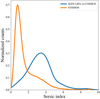 |
Fig. C.1. Distribution of Sérsic indices of luminous red sequence galaxies selected in GAMA-G10 (blue) versus that of all galaxies in the COSMOS Structure and Morphology catalogue (orange). The selected red sequence galaxies tend to have larger values of Sérsic indices compared to all galaxies in the COSMOS region. |
All Tables
All Figures
|
Fig. 1. Distribution of the selected luminous red sequence galaxies in colour space as a function of redshift (colour map). The COSMOS-G10 galaxies are shown as red stars. In each panel, the colour scale denotes the number density of luminous red galaxies in the colour-redshift space, with yellow corresponding to higher number densities and blue corresponding to lower number densities. |
| In the text | |
|
Fig. 2. Demonstration of the use of optical+NIR colours for the identification of likely stellar objects amongst the red sequence galaxy candidates. In each panel, the points colour-coded with redshift show the red sequence candidates in the (r − Ks)×(r − Z) space, while the blue contours show the 68% and 95% confidence regions of the distribution of stars with a high level of confidence. Left panel: at high redshifts (zred > 0.6), the considerable overlap between the distribution of red sequence candidates in the dense sample (L > 0.5 Lpivot(z)) and that of the high confidence stars becomes clear. Right panel: in the case of the red sequence candidates in the luminous sample (L > Lpivot(z)), the overlap between the two distributions is less apparent. |
| In the text | |
|
Fig. 3. Assessment of the purity of the red-sequence samples. At redshifts above zred > 0.4 red sequence galaxies (shown in red) and high confidence stars (shown in blue) reside in separated regions of the 2D (r − Ks)×(r − Z) colours, shown in the left panel. Shown by a pink dashed line is the predicted decision boundary between the two classes. The red sequence candidates falling below the predicted boundary are marked by open circles. These objects are flagged as likely stellar objects in the final catalogue, and thus removed from our large-scale structure analysis. Purity fraction of the dense (green dashed line) and the luminous (orange dashed line) samples as a function of redshift, in the right panel. |
| In the text | |
|
Fig. 4. Comparison between the estimated red sequence redshifts and spectroscopic redshifts for galaxies with spectroscopy. |
| In the text | |
|
Fig. 5. Distribution of the quantity (zspec − zred)/σz for the second redshift bin is shown in orange, where zred and σz are per galaxy estimated quantities. In blue: best-fit Student-t distribution. In red: best-fit Gaussian distribution. The Student t-distribution provides a better description of the long tails of the redshift distributions of individual galaxies. |
| In the text | |
|
Fig. 6. Redshift distributions of the four redshift bins designed for studying the large-scale structure. Shaded regions mark the redshift boundaries used for defining the redshift bins. |
| In the text | |
|
Fig. 7. Red sequence redshift (zred) distribution of the four redshift bins designed for studying the large-scale structure. |
| In the text | |
|
Fig. 8. HEALPIX maps of the density of Gaia DR2 stars with 14 < G < 17 in the KiDS DR4 footprint (first row), galactic dust extinction (second row), detection threshold above background (third row), and residual background (fourth row). All maps were generated with nside = 256. |
| In the text | |
|
Fig. 9. Demonstration of the correlation between some of the survey properties. In each panel, the mean and scatter values of the survey property indicated in the label of the y-axis are shown in bins of the survey property indicated in the label of the x-axis. The anti-correlation between the residual background counts in the coadds and the stellar number density is evident (left). There is an anti-correlation between the limiting magnitude in the r-band and the PSF FWHM r-band (middle). Furthermore, there is a correlation between the NIR magnitude limits in the H and the Ks bands (right). |
| In the text | |
|
Fig. 10. Relation between the set of orthogonal survey features |
| In the text | |
|
Fig. 11. Variation of the galaxy overdensity versus the orthogonal survey property parameters {S⊥} in the third redshift bin zred ∈ [0.45, 0.6], with (in blue) and without (in red) the photometric weights included. The deviation of the galaxy over density from unity is quantified by |
| In the text | |
|
Fig. 12. Clustering measurements for the four redshift bins. In each panel, the blue (orange) data points correspond to the correlation functions computed with (without) the photometric weights designed to remove survey-related systematic density variations. |
| In the text | |
|
Fig. 13. Comparison between the posterior predictions (red shaded) of clustering and the clustering measurements (blue points with error bars) in the four redshift bins. The dark and light shaded regions mark the 68% and the 95% confidence intervals. The error bars are derived from the diagonal elements of the covariance matrix of the observations. |
| In the text | |
|
Fig. 14. Joint constraints on the linear galaxy bias and photo-z shift parameters shown for the redshift bins constructed with the dense sample (blue contours) and the last redshift bin which is constructed from the luminous sample (red contour). |
| In the text | |
|
Fig. 15. Redshift dependence of the estimated linear galaxy bias shown for the dense sample (blue) and the luminous sample (red). The boxes mark the 68% and the 95% confidence intervals of the marginalised distribution over bias parameters. The solid (dashed) lines show the predictions of the passive evolution model of Fry (1996) given the bias constraints in the three redshift bins (in the last redshift bin) for each galaxy sample. |
| In the text | |
|
Fig. C.1. Distribution of Sérsic indices of luminous red sequence galaxies selected in GAMA-G10 (blue) versus that of all galaxies in the COSMOS Structure and Morphology catalogue (orange). The selected red sequence galaxies tend to have larger values of Sérsic indices compared to all galaxies in the COSMOS region. |
| In the text | |
Current usage metrics show cumulative count of Article Views (full-text article views including HTML views, PDF and ePub downloads, according to the available data) and Abstracts Views on Vision4Press platform.
Data correspond to usage on the plateform after 2015. The current usage metrics is available 48-96 hours after online publication and is updated daily on week days.
Initial download of the metrics may take a while.