| Issue |
A&A
Volume 674, June 2023
|
|
|---|---|---|
| Article Number | L13 | |
| Number of page(s) | 8 | |
| Section | Letters to the Editor | |
| DOI | https://doi.org/10.1051/0004-6361/202346935 | |
| Published online | 20 June 2023 | |
Letter to the Editor
First detection of the HSO radical in space⋆
1
Observatorio Astronómico Nacional (IGN), C/ Alfonso XII 3, 28014 Madrid, Spain
e-mail: This email address is being protected from spambots. You need JavaScript enabled to view it.
2
Observatorio de Yebes (IGN), Cerro de la Palera s/n, 19141 Yebes, Guadalajara, Spain
3
Dipartimento di Chimica “Giacomo Ciamician”, Universitá di Bologna, Via F. Selmi 2, 40126 Bologna, Italy
4
Grupo de Astrofísica Molecular, Instituto de Física Fundamental, CSIC, C/ Serrano 123, 28006 Madrid, Spain
Received:
18
May
2023
Accepted:
5
June
2023
Abstract
We report the discovery of HSO towards several cold dark clouds. The detection is confirmed by the observation of the fine and hyperfine components of two rotational transitions in the protostellar core B1-b, using the Yebes 40 m and IRAM 30 m telescopes. Furthermore, all the fine and hyperfine components of its fundamental transition 10, 1 − 00, 0 at 39 GHz were also detected toward the cyanopolyyne peak of TMC-1. The measured frequencies were used to improve the molecular constants and predict more accurate line frequencies. We also detected the strongest hyperfine component of the 10, 1 − 00, 0 transition of HSO toward the cold dark clouds L183, L483, L1495B, L1527, and Lupus-1A. The HSO column densities were obtained using LTE models that reproduce the observed spectra. The rotational temperature was constrained to 4.5 K in B1-b and TMC-1 using the available Yebes 40 m and IRAM 30 m data. The obtained column densities range between 7.0×1010 cm−2 and 2.9×1011 cm−2, resulting in abundances in the range of (1.4–7.0) × 10−12 relative to H2. Our observations show that HSO is widespread in cold dense cores. However, more observations, together with a detailed comparison with other S-bearing species, are needed to constrain the chemical production mechanisms of HSO, which are not considered in current models.
Key words: astrochemistry / ISM: abundances / ISM: clouds / ISM: molecules / line: identification
Based on observations with the 40m radio telescope of the National Geographic Institute of Spain (IGN) at Yebes Observatory (projects 19A003, 20A014, 20A016, 20D023, 21A006, 21A010, 21A011, 21D005, and 22B023), and the IRAM 30m telescope. Yebes Observatory thanks the ERC for funding support under grant ERC-2013-Syg-610256-NANOCOSMOS. IRAM is supported by INSU/CNRS (France), MPG (Germany) and IGN (Spain).
© The Authors 2023
 Open Access article, published by EDP Sciences, under the terms of the Creative Commons Attribution License (https://creativecommons.org/licenses/by/4.0), which permits unrestricted use, distribution, and reproduction in any medium, provided the original work is properly cited.
This article is published in open access under the Subscribe to Open model. This email address is being protected from spambots. You need JavaScript enabled to view it. to support open access publication.
1. Introduction
Among the ∼300 molecules detected in space, 33 are sulfur-bearing species1, which makes sulfur an important and ubiquitous constituent of the interstellar medium (ISM). Furthermore, sulfur is a biogenic element and as such it is a fundamental constituent of life on Earth (Todd 2022). In spite of its importance, there are many unknowns in the chemical evolution of sulfur along the lifecycle of matter. One of the main issues raised in recent years is the missing sulfur problem. While in the diffuse ISM, the observed abundance of sulfur is found to be similar to the solar one (Goicoechea & Cuadrado 2021), in the cold and dense molecular clouds, the sum of the abundances of all detected S-bearing molecules accounts only for less than 1% of the sulfur (Vidal et al. 2017). The open question to consider is thus whether the missing sulfur is in the form of some gaseous species that has not yet been identified or whether it is present as some solid compound in dust grains.
The QUIJOTE2 line survey (Cernicharo et al. 2021a) has provided the detection of many new sulfur-bearing molecules in the dense core TMC-1 (Cernicharo et al. 2021b,c; Cabezas et al. 2022; Fuentetaja et al. 2022). It is likely that these molecules are also present in other molecular clouds, but still their abundances do not account for the missing sulfur. In the past, other species have been the target of astronomical searches in order to find the main sulfur reservoir, but without success. One of them is HSO, which was searched for by Cazzoli et al. (2016), based on the accurate laboratory investigation of its rotational spectrum up to the THz region. These authors targeted the massive star-forming regions, Orion KL and Sgr B2, as well as the dense core B1-b in various transitions lying at 1, 2, and 3 mm, but did not detect HSO. However, they did not use the most favorable transitions, at least for the cold dense core B1-b, which lie at lower frequencies. Here, we present new data towards B1-b, obtained with the Yebes 40 m and IRAM 30 m telescopes, where we have identified HSO. Using the very deep spectral line survey QUIJOTE, performed with the Yebes 40 m telescope, we have also detected all the fine and hyperfine components of the 10, 1 − 00, 0 rotational transition of HSO towards the cyanopolyyne peak of TMC-1 (hereafter TMC-1 CP). Moreover, we also report the detection of HSO toward five additional cold dense cores.
2. Observations
The data of B1-b and TMC-1 CP presented here are part of the spectral line surveys performed at the Yebes 40 m and IRAM 30 m telescopes. The Yebes 40 m data at 7 mm cover the full Q band, between 31.1 GHz and 50.4 GHz, using the NANOCOSMOS HEMT Q band receiver (Tercero et al. 2021) and the fast Fourier transform spectrometers (FFTS), which allow almost the full coverage of the band at a spectral resolution of 38 kHz. We observed two setups at different central frequencies in order to fully cover the lower and upper frequencies allowed by the Q band receiver and to check for spurious signals and other technical artifacts. The Yebes 40 m data of TMC-1 CP correspond to the QUIJOTE deep spectral survey, see Cernicharo et al. (2021a, 2023) for details. The observations of B1-b were performed in different projects, in January and February 2020 and between June and August 2021. The IRAM 30 m data consist of a 3 mm line survey that covers the full available band at the telescope, between 71.6 GHz and 117.6 GHz, using the EMIR 090 receiver connected to the FTS in its narrow mode, which provides a spectral resolution of 49 kHz and a total bandwidth of 7.2 GHz. Observations were performed in several runs. Between January and May 2012, we completed the scan 82.5–117.6 GHz (see Cernicharo et al. 2012), and in August 2018, after the upgrade of the E090 receiver, we extended the survey down to 71.6 GHz. More recent observations in 2021 from other projects at 3 mm, which cover transitions of HSO between 75 and 81 GHz, have been used to complement the data and confirm or provide improved upper limits.
Additional Yebes 40 m data at 7 mm of the dense cores L183, L483, L1495B, L1527, and Lupus-1A are also included in this Letter. The observing strategy was similar to that used for B1-b and TMC-1 CP, although the total observing time dedicated to each source is uneven.
For both the Yebes 40 m and IRAM 30 m telescopes, observations were performed using the frequency switching technique. The intensity scale in the spectra is  , antenna temperature corrected for atmospheric absorption and spillover losses, which was calibrated using two absorbers at different temperatures and the atmospheric transmission model ATM (Cernicharo 1985; Pardo et al. 2001). The estimated uncertainty for
  is 10%. At the observed frequencies, the main beam efficiency is 0.58 and 0.82 for the 40 m and 30 m telescopes, respectively, and the half power beam width (HPBW) is 44″ and 31″ at 39 GHz and 79 GHz, respectively. All the data were reduced and analyzed using the GILDAS3 software.
3. Results
3.1. Line identification
During the analysis of the 7 mm line survey of B1-b, we detected a series of nearby unidentified lines around 39.5 GHz. Using the Cologne Database for Molecular Spectroscopy (CDMS, Müller et al. 2005) and the MADEX4 code (Cernicharo et al. 2012), where the predictions for the line frequencies were obtained from the rotational constants of Cazzoli et al. (2016), we assigned the observed lines to the N = 10, 1 − 00, 0 rotational transition of HSO. This transition shows multiple fine and hyperfine components due to electron and nuclear (of hydrogen) spins hyperfine interactions. All of them were detected in the B1-b spectra. We also searched for other transitions within the 3 mm IRAM survey, where the strongest components of the N = 20, 2 − 10, 1 transition were also identified towards B1-b (see Fig. 1). In TMC-1 CP, all the components of the N = 10, 1 − 00, 0 rotational transition of HSO were clearly detected, thanks to the very high sensitivity of the QUIJOTE 7 mm survey data (see Fig. 2). However, no lines were detected at 3 mm.
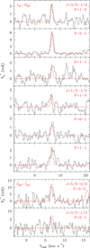 |
Fig. 1. Observed transitions of HSO toward B1-b with the Yebes 40 m (upper panels) and the IRAM 30 m (bottom panels) telescopes. The red line shows the LTE synthetic spectrum obtained from a fit to the observed line profiles (see text). Note: the 20, 2 − 11, 0, J = 5/2–3/2, F = 2–1 component, shown in the LTE model to the right of the bottom panels, is blended with a negative artifact resulting from the frequency switching observing technique. The observed position in B1-b is αJ2000 = 03h33m20.8s and δJ2000 = 31° 07′34.0″. |
Table 1 shows the observed parameters obtained from Gaussian fits for both sources, where we also include 3σ upper limits for non-detections. From the Gaussian fits, we noticed some differences in the measured frequencies in the spectra. The latter were obtained using a fixed local standard of rest velocity value for each source. For TMC-1 CP the velocity used is 5.83 km s−1, obtained from other molecules within the QUIJOTE line survey (Cernicharo et al. 2020). B1-b shows two velocity components for some molecules, at 6.5 and 7.0 km s−1, therefore we used the averaged value of 6.70 km s−1, obtained from fits to multiple molecular species, which has been used in previous studies (see, e.g., Marcelino et al. 2005). We used the observed frequencies in TMC-1 CP, where the LSR velocity is better determined and lines are narrower, to improve the molecular constants and obtain new rest frequencies (see Sect. 3.2 for details of the new calculations). Table A.1 shows the new calculated frequencies and line parameters of the observed transitions, while in Table 1 we show the difference between the observed frequency and the new calculated rest frequency.
Line parameters of the detected transitions of HSO.
The HSO lines at 3 mm have only been detected towards B1-b, where the strongest component of the 20, 2 − 10, 1 transition is clearly seen. However, the J = 3/2–1/2 F = 2–1 component at 79 378 MHz is at the limit of detection, with a S/N of only 2.5 (see Fig. 1 and Table 1). Another HSO component that is similar in intensity, at 79 162 MHz, is blended with a negative artifact produced by the folding of the frequency-switching spectra (see Fig. 1). There are other HSO lines covered in the 3 mm survey that have been searched for in B1-b, but they are not detectable due to the high energy levels involved and low expected intensities. Among them is the 21, 1 − 11, 0 transition at 81.3 GHz searched for by Cazzoli et al. (2016) towards B1-b, with an upper level energy of 19.1 K. While the new survey data gathered in 2018 improved the sensitivity of the spectra, no line was detected with a root mean square (rms) of ∼3 mK. Thanks to the extension of the B1-b survey below 80 GHz, we were able to access the more favourable rotational transitions detected in this work.
In addition, HSO has also been identified in other dense cores observed by our group with the Yebes 40 m and the IRAM 30 m telescopes (Marcelino et al., in prep.; Agúndez et al., in prep.). We have detected the strongest component of the N = 10, 1 − 00, 0 transition towards L183, L483, L1495B, Lupus-1A, and (tentatively) in L1527. Figure A.1 shows the observed line profiles, where the calculated frequency is indicated by a vertical dashed line. There are slight deviations from the calculated frequencies in some of the cores, which are mostly within the full width at high maximum (FWHM) of the lines. However, the line in L1527 shows a significant difference. We searched the molecular catalogs for other possible carriers for this line in L1527, but could not find any other than HSO. Yoshida et al. (2019), in their Nobeyama spectral survey, also observed variations in the observed velocity for some lines, up to 0.6 km s−1, compatible with the deviation we also found for HSO. Nevertheless, we still consider the detection in L1527 as tentative. Table 1 shows the obtained line parameters and upper limits for all the sources. In L183, we also identified two other components of the N = 10, 1 − 00, 0 transition, while no other lines have been detected in the rest of the cores. It is worth noting that although these cores show stronger HSO line intensities than TMC-1 CP, we could detect all the hyperfine components of the N = 10, 1 − 00, 0 transition in TMC-1 CP thanks to the very high sensitivity of the QUIJOTE survey. Our 30 m observations only cover the N = 20, 2 − 10, 1 transition for L483, where the full band was observed in the spectral line survey performed by Agúndez et al. (2019). However, no line was detected. Indeed, from our local themodynamical equilibrium (LTE) models (see Sect. 3.3), we obtained an expected value for the intensity of the strongest component at 79 165 MHz, namely, of ∼4 mK, which is consistent with a non-detection (see Table 1).
3.2. Improved molecular constants for HSO
The HSO radical (2A″) is a prolate asymmetric top belonging to Hund’s case b, with J = N + S and F = J + I, where N, S, and J are the rotational angular momentum, electronic spin momentum, and total angular momentum, respectively. We note that I, the nuclear spin angular momentum of hydrogen, is coupled with N. Therefore, the effective Hamiltonian operator incorporates, in addition to the rotational Hamiltonian (also including centrifugal-distortion terms), two further terms: one describing the electron spin-rotation interaction (through the electron spin-rotation tensor ϵ) and the other one accounting for the nuclear hyperfine interactions (through isotropic Fermi-contact interaction constant aF and the anisotropic T tensor). Hydrogen (I = 1/2) is the only nucleus contributing to the nuclear hyperfine Hamiltonian, which also includes the almost negligible nuclear spin-rotation interaction (described through the C tensor). For further details, we refer, for instance, to Endo et al. (1981) and Cazzoli et al. (2016).
The rotational spectrum of HSO has been investigated in the laboratory by Endo et al. (1981) in the 79–161 GHz range and by Cazzoli et al. (2016) in the 194 GHz–1.2 THz interval. In the latter work, the two set of measurements were merged in a global fit, which was performed using the SPFIT/SPCAT suite of programs (Pickett 1991) and employing Watson’s S-reduced Hamiltonian (Watson 1977) in its Ir representation (Gordy & Cook 1984). In the global fit, each transition was weighted proportionally to the inverse square of its experimental uncertainty. The spectroscopic analysis was also supported by high-level quantum-chemical calculations (see Cazzoli et al. 2016, for all details). The line catalog obtained in Cazzoli et al. (2016) guided the present radioastronomical observations and led to the unequivocal detection of the hyperfine components of the N = 10, 1 − 00, 0 transition. However, their rest frequencies were predicted with uncertainties of about 200–300 kHz. Therefore, their incorporation in the global fit allowed us to improve the spectroscopic parameters. The results of this fit are compiled in Table A.2, where a comparison with the parameters from Cazzoli et al. (2016) is reported. The improvement is apparent and one additional octic centrifugal distortion constant (LKKN) has been determined in this study, which was excluded from the original fit because it was only barely determined. As expected, its incorporation has some impact on the HNK and HKN sextic terms as well as on the LNK octic parameter. Overall, the rms error increased from 0.9 (Cazzoli et al. 2016) to 1.1 (the present work). This slight worsening is not related to centrifugal distortion, but to the new detected transitions in B1-b and TMC-1 CP. Indeed, the two sets of frequencies differ one from the other by more than the assigned uncertainties.
3.3. Column densities
The new spectroscopic constants and frequencies of HSO were introduced in MADEX, which was used to produce LTE synthetic spectra. The comparison between the synthetic and the observed spectra allowed us to estimate the column density of HSO in each source. We used the dipole moments calculated by Cazzoli et al. (2016), μa = 2.18 D and μb = 0.65 D. We note that only a-type transitions were observed. Although the N = 20, 2 − 10, 1 transition was only detected towards B1-b, through only two hyperfine components, we used the 3 mm spectra in both TMC-1 CP and B1-b at the frequencies where an HSO line is expected to constrain the rotational temperature and to check that the non-detections are consistent with the model predictions. The model takes into account the different telescope beams and efficiencies to obtain antenna temperature intensities for each line. We assumed uniform sources with a diameter size of 80″ for TMC-1 CP (Fossé et al. 2001) and 100″ for B1-b (Bachiller & Cernicharo 1984; Hirano et al. 1999), and linewidths of 1.0 km s−1 and 0.8 km s−1 for B1-b and TMC-1 CP, respectively, which are around the average value obtained from the Gaussian fits to the HSO lines. The rotational temperature that better reproduces the observed spectra from both the Yebes 40 m and IRAM 30 m telescopes is 4.5 K. This value is lower than the kinetic temperature usually obtained for B1-b and TMC-1 CP, ∼10 K (see, e.g., Marcelino et al. 2005, 2009). However, values higher than 5 K overestimate the 3 mm data. Figures 1 and 2 show the synthetic spectra from the LTE models in red, overlaid with the observed line profiles. We used the same rotational temperature of 4.5 K to compute an LTE model for the other cores where HSO has been detected. We assumed that all the sources are extended (see, e.g., Sakai et al. 2010a; Cordiner et al. 2013) and used a source size of 100″ in our models, which is more than twice the beam of the Yebes 40 m telescope at the frequencies of HSO. Frequencies and linewidths used in the models are obtained from the Gaussian fits (see Table 1). Figure A.1 shows the LTE models overlaid with the spectra and Table 2 gives the obtained column densities and abundances for all the sources.
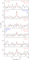 |
Fig. 2. Observed transitions of HSO toward TMC-1 CP, from the Yebes 40 m QUIJOTE survey. The red line shows the LTE synthetic spectrum obtained from a fit to the observed line profiles (see text). The observed position of TMC-1 CP is αJ2000 = 4h41m41.9s and δJ2000 = +25° 41′27.0″. |
Obtained column densities and abundances for HSO.
The highest HSO column density was obtained for B1-b, where the strongest lines have been observed. This value is significantly higher than in TMC-1 CP, while for the other dense cores, we found values in the range of (1–2) × 1011 cm−2. The errors in the column densities are estimated to be 20% in B1-b and TMC-1 CP, where we observed a larger number of lines and the spectra are more sensitive, and the errors are 50% for the other sources. We adopted H2 column densities from the literature to derive fractional abundances of HSO to improve the comparison of the results from the observed cores (see Table 2). The fractional abundances of HSO are similar among the sources, with values in the range of (1.4–4.3) × 10−12 relative to H2, the only exception being TMC-1 CP, which has the highest HSO abundance, 7×10⁻¹² relative to H2. However, the fractional abundances are affected by the different methods used to obtain the H2 column density and, therefore, we consider that HSO is present in these cold dense cores, with similar abundances of a few times 10−12 relative to H2.
4. Discussion
The rotational temperatures obtained from the LTE models in B1-b and TMC-1 CP indicate that HSO emission arises from a cold region in the clouds. It is known, however, that B1-b has two very young embedded sources: B1-bN, a first hydrostatic core candidate, and B1-bS, an extremely young Class 0 protostar (Gerin et al. 2015). In fact, ALMA observations by Marcelino et al. (2018) show that B1-bS contains a hot and compact region with strong emission from complex organic molecules (COMs). The emission from these species was reproduced by using a source model with two components, one very compact and hot (200 K and 0.35″) and another one at lower temperature (60 K and 0.6″). We explored the possibility that the emission from HSO could arise from such compact and warm regions. We ran a series of LTE models with temperatures between 60 and 200 K, where we changed the column density and the source size. We could not find any solution reproducing the observed line profiles from the two telescopes. Furthermore, we did not detect other transitions in the 3 mm data involving higher energy levels (see also Cazzoli et al. 2016). Therefore, the HSO emission in B1-b should arise from the cold envelope.
The low temperature of 4.5 K obtained from the observed spectra in B1-b and TMC-1 CP is consistent with those obtained for SO by Loison et al. (2019) in the same sources. From rotation diagrams, these authors obtained temperatures of 6.5±0.7 K and 3.9±0.1 K for B1-b and TMC-1 CP, respectively. The rotational temperature obtained in TMC-1 CP is actually very similar to the one calculated for HSO from our LTE models, which could indicate a common origin. Among the other observed dense cores, L483 and L1527 have been considered as warm carbon-chain chemistry sources (Sakai et al. 2008; Oya et al. 2017). In fact, the kinetic temperature in L1527 has been found to be 13.9 K (Sakai et al. 2008), which is slightly higher than 10 K. However, in both L483 and L1527, the rotational temperature of SO is low, at 4.5 K and 6 K, respectively (Agúndez et al. 2019; Yoshida et al. 2019), which supports the use of a low rotational temperature for HSO in these sources. Table 2 shows the abundance ratio N(HSO)/N(SO) using SO column densities from the literature. It is seen that this ratio is not uniform across the different sources, but it exhibits large variations from one source to another. This behavior may hold information on the chemistry of HSO, which is as yet poorly constrained. We note that the highest ratios are found for L1527 and TMC-1 CP, both known for their high abundance in carbon chain molecules.
Our results show that HSO is indeed present in cold gas. However, HSO was not detected by Cazzoli et al. (2016) towards the high-mass star forming regions Orion KL and Sgr B2. These authors obtained upper limits to the column density of ∼1×1014 cm−2, for both Orion KL and Sgr B2(N), including the cold gas component for the latter, where the N = 101 − 000 transition at 39 GHz was not detected in the PRIMOS5 data. Since they did not detect HSO in their search, including B1-b, Cazzoli et al. (2016) concluded that HSO does not achieve a significant abundance to be detectable in these clouds. However, although the observed abundances of HSO, of a few times ∼10−12 relative to H2, are too low to account for the missing sulfur in molecular clouds, our results show that HSO is a widespread molecule in cold regions. Further investigation is needed to elucidate whether HSO could be observed in other type of interstellar sources, such as diffuse clouds. Furthermore, the chemistry of HSO has not been explored in current chemical models. The formation pathways to the HSO radical in cold interstellar clouds are quite uncertain (Cazzoli et al. 2016). This species is not included in either the UMIST (McElroy et al. 2013) or KIDA (Wakelam et al. 2015) chemical kinetics databases. Neutral–neutral reactions, such as O + H2S, O2 + SH, or O + CH3SH, have barriers when leading to HSO or are endothermic processes (Tsuchiya et al. 1994, 1997; Cardoso et al. 2012). The OH + SH reaction is an interesting possibility, although to the best of our knowledge, it has not yet been studied. Alternatively, HSO could be produced from the dissociative recombination of ions such as H2SO+, although the chemistry of this cation is currently unexplored in chemical networks.
5. Conclusions
We report the detection of a new molecule, HSO, towards several cold dark clouds. Furthermore, thanks to the deep observations from the Yebes 40 m telescope, we detected all the fine and hyperfine components of the N = 10, 1 − 00, 0 transition towards B1-b and TMC-1 CP. The latter was used to improve the spectroscopic molecular constants and frequencies of HSO. The detection of the strongest component of this transition towards other dense cores demostrates that HSO is widespread in cold environments, despite its low abundance. Although HSO is a simple molecule with common atoms, its chemistry has not been studied in detail. Further observations are needed to investigate whether these species could be produced under different conditions.
Q-band Ultrasensitive Inspection Journey to the Obscure TMC-1 Environment.
PRebiotic Interstellar MOlecule Survey https://www.cv.nrao.edu/PRIMOS/index.html
Acknowledgments
We acknowledge funding support from Spanish Ministerio de Ciencia e Innovación through grants PID2019-106110GB-I00, PID2019-107115GB-C21, and PID2019-106235GB-I00, and from the European Research Council (ERC Grant 610256: NANOCOSMOS).
References
- Agúndez, M., Marcelino, N., Cernicharo, J., Roueff, E., & Tafalla, M. 2019, A&A, 625, A147 [Google Scholar]
- Bachiller, R., & Cernicharo, J. 1984, A&A, 140, 414 [NASA ADS] [Google Scholar]
- Cabezas, C., Agúndez, M., Marcelino, N., et al. 2022, A&A, 657, L4 [NASA ADS] [CrossRef] [EDP Sciences] [Google Scholar]
- Cardoso, D., Ferrão, L., Spada, R., Roberto Neto, O., & Machado, F. 2012, Int. J. Quant. Chem., 112 [Google Scholar]
- Cazzoli, G., Lattanzi, V., Kirsch, T., et al. 2016, A&A, 591, A126 [NASA ADS] [CrossRef] [EDP Sciences] [Google Scholar]
- Cernicharo, J. 1985, Internal IRAM Report (Granada: IRAM) [Google Scholar]
- Cernicharo, J. 2012, in EAS Publications Series, eds. C. Stehlé, C. Joblin, & L. d’Hendecourt, 58, 251 [NASA ADS] [CrossRef] [EDP Sciences] [Google Scholar]
- Cernicharo, J., & Guelin, M. 1987, A&A, 176, 299 [NASA ADS] [Google Scholar]
- Cernicharo, J., Marcelino, N., Roueff, E., et al. 2012, ApJ, 759, L43 [NASA ADS] [CrossRef] [Google Scholar]
- Cernicharo, J., Marcelino, N., Agúndez, M., et al. 2020, A&A, 642, L8 [NASA ADS] [CrossRef] [EDP Sciences] [Google Scholar]
- Cernicharo, J., Agúndez, M., Kaiser, R. I., et al. 2021a, A&A, 652, L9 [NASA ADS] [CrossRef] [EDP Sciences] [Google Scholar]
- Cernicharo, J., Cabezas, C., Agúndez, M., et al. 2021b, A&A, 648, L3 [EDP Sciences] [Google Scholar]
- Cernicharo, J., Cabezas, C., Endo, Y., et al. 2021c, A&A, 650, L14 [NASA ADS] [CrossRef] [EDP Sciences] [Google Scholar]
- Cernicharo, J., Pardo, J. R., Cabezas, C., et al. 2023, A&A, 670, L19 [NASA ADS] [CrossRef] [EDP Sciences] [Google Scholar]
- Cordiner, M. A., Buckle, J. V., Wirström, E. S., Olofsson, A. O. H., & Charnley, S. B. 2013, ApJ, 770, 48 [NASA ADS] [CrossRef] [Google Scholar]
- Crapsi, A., Caselli, P., Walmsley, C. M., et al. 2005, ApJ, 619, 379 [Google Scholar]
- Endo, Y., Saito, S., & Hirota, E. 1981, J Cosmology Phys., 75, 4379 [Google Scholar]
- Fossé, D., Cernicharo, J., Gerin, M., & Cox, P. 2001, ApJ, 552, 168 [Google Scholar]
- Fuentetaja, R., Agúndez, M., Cabezas, C., et al. 2022, A&A, 667, L4 [NASA ADS] [CrossRef] [EDP Sciences] [Google Scholar]
- Gerin, M., Pety, J., Fuente, A., et al. 2015, A&A, 577, L2 [NASA ADS] [CrossRef] [EDP Sciences] [Google Scholar]
- Goicoechea, J. R., & Cuadrado, S. 2021, A&A, 647, L7 [NASA ADS] [CrossRef] [EDP Sciences] [Google Scholar]
- Gordy, W., & Cook, R. L. 1984, Microwave Molecular Spectra (New York: Wiley) [Google Scholar]
- Hirano, N., Kamazaki, T., Mikami, H., Ohashi, N., & Umemoto, T. 1999, in Star Formation 1999, ed. T. Nakamoto, 181 [Google Scholar]
- Hirota, T., Maezawa, H., & Yamamoto, S. 2004, ApJ, 617, 399 [Google Scholar]
- Lattanzi, V., Bizzocchi, L., Vasyunin, A. I., et al. 2020, A&A, 633, A118 [NASA ADS] [CrossRef] [EDP Sciences] [Google Scholar]
- Loison, J.-C., Wakelam, V., Gratier, P., et al. 2019, MNRAS, 485, 5777 [Google Scholar]
- Marcelino, N., Cernicharo, J., Roueff, E., Gerin, M., & Mauersberger, R. 2005, ApJ, 620, 308 [NASA ADS] [CrossRef] [Google Scholar]
- Marcelino, N., Cernicharo, J., Tercero, B., & Roueff, E. 2009, ApJ, 690, L27 [CrossRef] [Google Scholar]
- Marcelino, N., Gerin, M., Cernicharo, J., et al. 2018, A&A, 620, A80 [NASA ADS] [CrossRef] [EDP Sciences] [Google Scholar]
- McElroy, D., Walsh, C., Markwick, A. J., et al. 2013, A&A, 550, A36 [NASA ADS] [CrossRef] [EDP Sciences] [Google Scholar]
- Müller, H. S. P., Schlöder, F., Stutzki, J., & Winnewisser, G. 2005, J. Mol. Struct., 742, 215 [Google Scholar]
- Oya, Y., Sakai, N., Watanabe, Y., et al. 2017, ApJ, 837, 174 [Google Scholar]
- Pardo, J. R., Cernicharo, J., & Serabyn, E. 2001, IEEE Trans. Anten. Propag., 49, 1683 [CrossRef] [Google Scholar]
- Pickett, H. M. 1991, J. Mol. Spectrosc., 148, 371 [Google Scholar]
- Sakai, N., Sakai, T., Hirota, T., & Yamamoto, S. 2008, ApJ, 672, 371 [Google Scholar]
- Sakai, N., Sakai, T., Hirota, T., Burton, M., & Yamamoto, S. 2009, ApJ, 697, 769 [Google Scholar]
- Sakai, N., Sakai, T., Hirota, T., & Yamamoto, S. 2010a, ApJ, 722, 1633 [Google Scholar]
- Sakai, N., Shiino, T., Hirota, T., Sakai, T., & Yamamoto, S. 2010b, ApJ, 718, L49 [NASA ADS] [CrossRef] [Google Scholar]
- Tercero, F., López-Pérez, J. A., Gallego, J. D., et al. 2021, A&A, 645, A37 [EDP Sciences] [Google Scholar]
- Todd, Z. R. 2022, Life, 12 [Google Scholar]
- Tsuchiya, K., Yokoyama, K., Matsui, H., Oya, M., & Dupre, G. 1994, J. Phys. Chem., 98, 8419 [CrossRef] [Google Scholar]
- Tsuchiya, K., Kamiya, K., & Matsui, H. 1997, Int. J. Chem. Kinet., 29, 57 [CrossRef] [Google Scholar]
- Vidal, T. H. G., Loison, J.-C., Jaziri, A. Y., et al. 2017, MNRAS, 469, 435 [Google Scholar]
- Wakelam, V., Loison, J. C., Herbst, E., et al. 2015, ApJS, 217, 20 [NASA ADS] [CrossRef] [Google Scholar]
- Watson, J. K. G. 1977, in Vibrational Spectra and Structure, ed. J. Durig (Amsterdam: Elsevier), 6, 1 [Google Scholar]
- Yoshida, K., Sakai, N., Nishimura, Y., et al. 2019, PASJ, 71, S18 [NASA ADS] [CrossRef] [Google Scholar]
Appendix A: Additional tables and figures
Transitions of HSO observed with the Yebes 40m and IRAM 30m telescopes.
Spectroscopic parametersa, b of HSO.
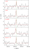 |
Fig. A.1. HSO N = 10, 1 − 00, 0J = 3/2 − 1/2 F = 2 − 1 transition observed in five cold dense cores with the Yebes 40m telescope. The abscissa corresponds to the rest frequency assuming the local standard of rest velocity for each source (see Table 1). The ordinate is the antenna temperature corrected for atmospheric losses in mK. The red line shows the LTE synthetic spectrum obtained from a fit to the observed line profiles (see text). The green vertical dashed line indicates the new calculated frequency corresponding with this transition. Observed positions for each source are: L183: αJ2000 = 15h54m08.6s and δJ2000 = −02° 52′10.0″, L483: αJ2000 = 18h17m29.83s and δJ2000 = −04° 39′38.33″, L1495B: αJ2000 = 04h15m41.8s and δJ2000 = 28° 47′46.0″, L1527: αJ2000 = 04h39m53.88s and δJ2000 = 26° 03′11.0″, and Lupus-1A: αJ2000 = 15h42m52.4s and δJ2000 = −34° 07′53.5″. |
All Tables
All Figures
|
Fig. 1. Observed transitions of HSO toward B1-b with the Yebes 40 m (upper panels) and the IRAM 30 m (bottom panels) telescopes. The red line shows the LTE synthetic spectrum obtained from a fit to the observed line profiles (see text). Note: the 20, 2 − 11, 0, J = 5/2–3/2, F = 2–1 component, shown in the LTE model to the right of the bottom panels, is blended with a negative artifact resulting from the frequency switching observing technique. The observed position in B1-b is αJ2000 = 03h33m20.8s and δJ2000 = 31° 07′34.0″. |
| In the text | |
|
Fig. 2. Observed transitions of HSO toward TMC-1 CP, from the Yebes 40 m QUIJOTE survey. The red line shows the LTE synthetic spectrum obtained from a fit to the observed line profiles (see text). The observed position of TMC-1 CP is αJ2000 = 4h41m41.9s and δJ2000 = +25° 41′27.0″. |
| In the text | |
|
Fig. A.1. HSO N = 10, 1 − 00, 0J = 3/2 − 1/2 F = 2 − 1 transition observed in five cold dense cores with the Yebes 40m telescope. The abscissa corresponds to the rest frequency assuming the local standard of rest velocity for each source (see Table 1). The ordinate is the antenna temperature corrected for atmospheric losses in mK. The red line shows the LTE synthetic spectrum obtained from a fit to the observed line profiles (see text). The green vertical dashed line indicates the new calculated frequency corresponding with this transition. Observed positions for each source are: L183: αJ2000 = 15h54m08.6s and δJ2000 = −02° 52′10.0″, L483: αJ2000 = 18h17m29.83s and δJ2000 = −04° 39′38.33″, L1495B: αJ2000 = 04h15m41.8s and δJ2000 = 28° 47′46.0″, L1527: αJ2000 = 04h39m53.88s and δJ2000 = 26° 03′11.0″, and Lupus-1A: αJ2000 = 15h42m52.4s and δJ2000 = −34° 07′53.5″. |
| In the text | |
Current usage metrics show cumulative count of Article Views (full-text article views including HTML views, PDF and ePub downloads, according to the available data) and Abstracts Views on Vision4Press platform.
Data correspond to usage on the plateform after 2015. The current usage metrics is available 48-96 hours after online publication and is updated daily on week days.
Initial download of the metrics may take a while.