| Issue |
A&A
Volume 674, June 2023
|
|
|---|---|---|
| Article Number | A104 | |
| Number of page(s) | 22 | |
| Section | Numerical methods and codes | |
| DOI | https://doi.org/10.1051/0004-6361/202245684 | |
| Published online | 09 June 2023 | |
Automatic line selection for abundance determinations in large stellar spectroscopic surveys★
1
Université Côte d’Azur, Observatoire de la Côte d’Azur, CNRS, Laboratoire Lagrange,
06000
Nice, France
e-mail: This email address is being protected from spambots. You need JavaScript enabled to view it.
2
Department of Astronomy, Stockholm University, AlbaNova University Centre,
106 91
Stockholm, Sweden
Received:
13
December
2022
Accepted:
17
February
2023
Abstract
Context. Over the past few years, new multiplex spectrographs have emerged to observe several millions of stars. The optimisation of these instruments (w.r.t. their resolution or wavelength range), their associated surveys (choice of instrumental set-up), and their parameterisation pipelines require methods that estimate which wavelengths (or pixels) contain useful information.
Aims. We propose a method that establishes the usefulness of an atomic spectral line, whereby usefulness is defined by the purity of the line and its detectability. We demonstrate two applications of our code: a) optimising an instrument by comparing the number of detected useful lines at a given wavelength range and resolution; and b) optimising the line list for a given set-up, in the sense of creating a golden subsample of the least-blended lines that are detectable at a range of signal-to-noise ratio values.
Methods. The method compares pre-computed normalised synthetic stellar spectra containing all of the elements and molecules with spectra solely containing the lines of specific elements. Then, the flux ratios between the full spectrum and the element spectrum are computed to estimate the line purities. The method automatically identifies: (i) the line’s central wavelength, (ii) its detectability based on its depth and a given signal-to-noise threshold, and (iii) its usefulness based on the purity ratio defined above.
Results. We applied this method to compare the three WEAVE high-resolution set-ups (blue: 404–465 nm, green: 473–545 nm, red: 595–685 nm) and find that the green+red set-up both allows us to measure more elements and contains more numerous useful lines. However, there is a disparity in terms of which elements are detected over each of the set-ups that we have characterised. We also studied the performances of high-resolution (R ~ 20 000) and low-resolution (R ~ 6000) spectra covering the entire optical wavelength range. Assuming a purity threshold of 60%, we find that the high-resolution set-up contains a much wealthier selection of lines, for any of the considered elements; whereas the low-resolution set-up displays a ‘loss’ of 50% to 90% of the lines (depending on the nucleosynthetic channel considered), even when the signal-to-noise ratio is increased.
Conclusions. The method presented here provides a vital diagnostic of where to focus to get the most out of a spectrograph. It is easy to implement for future instruments that have not yet determined their final configuration, as well as for pipelines that require line masks.
Key words: line: identification / techniques: spectroscopic / stars: abundances / Galaxy: abundances
Tables with identified lines from 300 to 1000 nm, and resolving powers of 3000, 6000, 20 000, 40 000 and 80 000, are only available at the CDS via anonymous ftp to cdsarc.cds.unistra.fr (130.79.128.5) or via https://cdsarc.cds.unistra.fr/viz-bin/cat/J/A+A/674/A104
© The Authors 2023
 Open Access article, published by EDP Sciences, under the terms of the Creative Commons Attribution License (https://creativecommons.org/licenses/by/4.0), which permits unrestricted use, distribution, and reproduction in any medium, provided the original work is properly cited.
This article is published in open access under the Subscribe to Open model. This email address is being protected from spambots. You need JavaScript enabled to view it. to support open access publication.
1 Introduction
The relative abundance ratios of atomic elements measured from the stellar photospheres hold key information for multiple fields in modern astrophysics, ranging from galaxy formation (e.g., Freeman & Bland-Hawthorn 2002) to stellar nucleosynthesis (Burbidge et al. 1957; Iwamoto et al. 1999; Nomoto et al. 2013; Karakas & Lattanzio 2014, and references therein), especially when coupled with an estimation of the stellar age (e.g. Kordopatis et al. 2023). More specifically, by measuring the elemental abundance pattern of a star, it is possible to determine its birthplace and siblings, as well as the star formation history that preceded its origin. However, measuring the abundance of specific elements in a stellar spectrum is not straightforward (e.g. Jofré et al. 2019). Ultimately, inferring the amount of atoms of a species present in the photosphere depends on how easily a specific spectral line is detectable, measurable, and transformable into an abundance value. In other words, this task depends on the accuracy of the stellar atmosphere and line profile modelling (Gray 2005) as well as, on the other hand, on how accurately the spectral line can be measured (signal-to-noise ratio, resolution of the spectrum, and blending together of several stellar features). The accuracy of the line modelling in turn depends on how accurately and precisely the stellar atmospheric parameters are known (i.e. the effective temperature, Teff, surface gravity, log g, global metallicity, [M/H], and α-element enhancement, [α/Fe]).
As a consequence, the design phase of a spectroscopic survey is a tough negotiation between spectral resolution, exposure time, adopted wavelength range, and total number of targets observed by the end of the project (e.g. Feltzing 2016). For this purpose, it is important to be able to easily assess early on what information is available at a given spectral range, resolving power (R = λ/Δλ), and signal-to-noise (S/N) for specific types of stars. This is intrinsically not trivial as it often requires that some kind of stellar spectra parameterisation pipeline is already available (e.g. Caffau et al. 2013; Bedell et al. 2014; Hansen et al. 2015). However, such a pipeline often requires a tedious phase of training and/or optimisation (e.g. Recio-Blanco et al. 2006; Kordopatis et al. 2011, 2013; Ness et al. 2015; Piskunov & Valenti 2017), which is therefore incompatible with the timescale or even the scope of the desired tests. In this context, recent years have seen the development of codes that quickly explore the available information in a spectrograph’s configuration, with the aim of providing answers to the above questions (e.g. Ruchti et al. 2016; Ting et al. 2017; Sandford et al. 2020).
The Spectral Wavelength Optimization Code (SWOC, Ruchti et al. 2016) requires the user to provide a predefined table containing the central wavelength and the equivalent width (or line depth) of features that are considered to be of particular interest. The SWOC then evaluates the quality and the wavelength distribution of these features for a considered stellar type, determines the optimal wavelength coverage based on a defined figure of merit, and eventually combines this information for different stellar types to ascertain the optimal wavelength coverage for a survey. This approach therefore relies on already having a priori information regarding which lines are of interest. This is not always the case, especially in wavelength regions that have not yet been commonly used in large surveys in the past.
A different approach was adopted by Ting et al. (2017) and Sandford et al. (2020), that employ the Cramér-Rao bound metric to quantify the amount of information available in a spectrum of specific wavelength range and resolution, associated with a given label (in this case, elemental abundance). As it is based on so-called gradient spectra, namely, the variation of the spectrum at a given wavelength associated to a specific label as well as on the covariance matrix of the spectrum, the metric sums over the different wavelength pixels to inform the user which elements can be detected above a given significance threshold. Ting et al. (2017) concluded that given a fixed exposure time and number of pixels (therefore different S/N and wavelength ranges depending on the resolution), low-resolution spectra could provide an equivalent amount of information to high-resolution spectra. However, this conclusion was obtained assuming that resolution and S/N values are uniform across the wavelength range and that line blends are correctly known (and modelled), which is often not the case.
The caveats mentioned in the previous paragraphs motivated the development of a new code, which is the focus of this paper. Its purpose is to identify ‘useful’ lines in a synthetic spectrum, namely, lines that are visible and not heavily blended at a given spectral resolution and S/N, without any a priori knowledge. This information is then stored and can be used to create either a line-list selection for spectral analysis (e.g. for abundance determination) or to visualise how many lines of a specific element or a nucleosynthetic channel are useful for a given instrumental configuration. It therefore has immediate and valuable applications for spectroscopic surveys based on already existing or future spectroscopic facilities or instruments such as APOGEE (Majewski et al. 2017), DESI (Abareshi et al. 2022), Gaia-RVS (Gaia Collaboration 2016; Cropper et al. 2018), GALAH (De Silva et al. 2015), LAMOST (Deng et al. 2012), 4MOST (de Jong et al. 2019), WEAVE (Jin et al. 2023), MOONS (Cirasuolo et al. 2020), MSE (The MSE Science Team 2019), PFS (Takada et al. 2014), and so on.
The paper is structured as follows. In Sect. 2, we present the concept of the code: details on how it runs, along with the required inputs and the outputs. The synthetic spectral library that the code relies on is described in Sect. 3. The application of the code is then described in Sect. 4, based on several examples. In Sect. 4.1 a verification of the identified lines based on the line list established within the Gaia-ESO survey (Randich et al. 2022; Gilmore et al. 2022) is performed. In Sect. 4.2, we show an illustration of how an instrument’s design can be optimised, by comparing the performances of high-and low-resolution spectrographs for specific types of stars. In Sect. 4.3, we evaluate the performance of the two WEAVE high-resolution configurations to suggest the set-up that can best drive Galactic archaeology studies. In Sect. 4.4, we show how our code can be used to create a ‘golden’ line list for spectral synthesis codes. Finally, we present our conclusions in Sect. 5.
2 Description of the code
2.1 The algorithm
We allow Sf,θ(λ) be the normalised synthetic spectrum of a star at a given set of atmospheric parameters θ ={Teff, log g, [M/H], [α/Fe]}. This spectrum is computed at an instrumental resolving power R = λ/FWHMinst (where FWHMinst is the full width at half maximum of the line spread function of the instrument) with a sampling, dx. Sf,θ contains the lines and blends of all of the elements and molecules present at the photosphere of the star.
Similarly, we let S Ε,θ(λ) be the normalised stellar spectrum containing only the lines associated to the element, E, at the same θ parameters, resolving power, R, pixel sampling, dx, and same continuous opacities as in Sf,θ(λ). Each element, E, has a reference line list1 {λV,E} associated to it (Piskunov et al. 1995; Ryabchikova et al. 2015), which is used for the computation of both Sf,θ(λ) and SE,θ(λ). For convenience, in the following, we omit the θ subscript when it is implicit. The steps of our algorithm aimed at identifying the lines for a given element E are as follows:
First, we detect all of the lines in S Ε(λ) by identifying their cores blindly. To achieve this, we search for the zero crossings in the derivative of S Ε(λ), without imposing any threshold in the flux (however, see below for more details). We let {λi} be the list containing the wavelengths of all the identified line-cores, i, of the element, E. The number of lines in {λi} is smaller or equal to the number of VALD entries in {λV}.
Next, we identify the true central wavelength {λc} of each line in {λi} by cross-matching {λi} with {λV}. Often, several VALD lines fall within one dx from the considered λi. In this case, we use the Boltzmann equation to evaluate which λV is the most prominent in the considered subset. In practice, we choose the line that is expected to be the strongest, ranking all candidate lines according to excitation energy and oscillator strength in the following way:
 (1)
(1)
where A is the number of atoms, Eχ is the excitation potential of the line, log(gƒ) is the logarithm of the oscillator-strength times the statistical weight of the parent energy level, and k is the Boltzmann constant2.
Then, for each item in {λc}, we evaluate S Ε(λc) and keep the lines that are deep enough to be detected at a given S/N. This criterion, derived in Appendix A, is defined as:
 (2)
(2)
where S/Nresol is the S/N per resolution element (see Appendix A for the formula with S/N per pixel). We note that the criterion is applied to the elemental spectrum, S E(λ) rather than to the observed total spectrum S f(λ). The reason for this choice is that we want to impose a criterion on the detectability of the line independently of its blend (or purity; see Eq. (4)).
In the next step, for each λc, we identify the blue-end, λb, and red-end, λr, of the line, defined as the first wavelengths bluewards and redwards, whereby:
 (3)
(3)
namely, these are the wavelengths at which the flux has reached x percent of the value it had at its core. We limit the search for λb and λr to λc ± 1.5 · FWHMinst. A value of x = 0.02 (i.e. 2%) has been empirically adopted.
Next, we define the purity factor p as:
 (4)
(4)
and then compute the purity for the entire line (pt), the blue-half (pb), and the red-half (pr). This is done because the line can be blended differently on its blue or red wing (see e.g. Fig. 1) and a line that is free of blend in one of its wings may still be very useful and reliable for abundance determinations (see discussion of how blending can affect the equivalent width measurements in Appendix B). The following ranges, λmin and λmax, are therefore adopted in Eq. (4):

Finally, we evaluate the number of pixels in the blue Nb and in the red Nr that are close to the continuum (S f(λ) > 0.9) within the adopted (λmin, λmax). This allows us to eventually flag the lines that have a purity above a determined arbitrary value, but that can nevertheless be difficult to detect because they are in the wings of stronger lines further away from λmin or λmax.
2.2 Input and output of the algorithm
In order to run, the code requires as an input (i) a synthetic spectrum that includes all the elements; (ii) a set of synthetic spectra with the atomic lines of only one element3 each time, computed at the same wavelength range, resolving power, and atmospheric parameters as the full spectrum; (iii) the reference line-list for each element that has been used to compute the spectra; (iv) an arbitrary S/Nresol threshold; and, finally, (v) the spectral resolving power of the instrument. The latter two parameters are used to evaluate the detectability of a line at a given S/N. The spectral resolving power is applied by convolving the simulated spectra (provided with infinite resolution) with a Gaussian of appropriate FWHM.
The code delivers, for a given element, E, a table containing the central wavelengths of the lines λc, the blue-ends λb, the red-ends λr, the three purity factors (pb, pr, pt), the depth of the line in the full spectrum S f(λc), the depth of the line in the element spectrum, S e(λc), the number of pixels in the blue, Nb, and the red, Nr, that have a flux close to the continuum. This information can later be used as desired to make summary or diagnostic plots – or to select ‘clean’ lines for codes that require such an input.
Figure 1 shows three cherry-picked examples of line identifications with our code for a Solar-like spectrum at R = 20 000. The total, blue and red purity factors are encapsulated in the figure, together with the central wavelength, λc, and the depth of the line for the element spectrum alone.
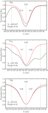 |
Fig. 1 Examples of identified lines for a Solar-like spectrum at R = 20 000. The elemental spectrum, i.e. the flux computed with the contribution from atomic lines from only one ionization stage of one element, is plotted in red. The full spectrum containing all of the elements and molecules is shown in black. The element and ionization stage associated to the line are noted on the upper left corner of each plot. The central wavelength of the identified line, λc is plotted as a vertical dashed grey line. The blue-end and the red-end of the line are plotted as vertical dashed green lines. The depth of the line in the element spectrum is indicated at the bottom left corner of each plot. The purity factor for the entire line is written at the middle-top of the plots. The blue-wing and red-wing purities are enclosed within the line at its left and right, respectively. |
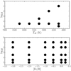 |
Fig. 2 Set of atmospheric parameters for which the full and elemental synthetic spectra were computed. |
3 Grid of synthetic spectra of infinite resolution
We consider nine stellar types, at different combinations of Teff and log g, along with six different values of [M/H] (see Fig. 2), resulting in 54 different templates.
The spectra are computed using PySME v4.104 (Wehrhahn et al. 2023) and the SME library v5.225 (Valenti & Piskunov 1996; Piskunov & Valenti 2017), together with the one-dimensional (1D) MARCS model atmospheres (Gustafsson et al. 2008), assuming local thermodynamic and hydrostatic equilibrium. The considered total wavelength range is λ = [300– 1000] nm. The sampling is constant at 8 × 10⁻⁵ nm. The adopted line list is from the VALD3 database (downloaded in January 2021). The molecular line-list includes CH, CN, C2, TiO, MgH, SiH, CO, and OH. The elemental abundance ratios are the same as for the MARCS model atmospheres, namely solar-scaled with Grevesse et al. (2007), except for Lithium (A(Li) = 2.00 adopted for all of the stars) and for α-elements, for which the abundance is a function of metallicity, as follows:
![Mathematical equation: $\matrix{ {\left[ {{\alpha \mathord{\left/ {\vphantom {\alpha {{\rm{Fe}}}}} \right. \kern-\nulldelimiterspace} {{\rm{Fe}}}}} \right] = + 0.4} & {\quad \quad {\rm{for}}\,\left[ {{{{\rm{Fe}}} \mathord{\left/ {\vphantom {{{\rm{Fe}}} {\rm{H}}}} \right. \kern-\nulldelimiterspace} {\rm{H}}}} \right] \le - 1.0} \cr } ,$](/articles/aa/full_html/2023/06/aa45684-22/aa45684-22-eq6.png) (5)
(5)
![Mathematical equation: $\matrix{ {\left[ {{\alpha \mathord{\left/ {\vphantom {\alpha {{\rm{Fe}}}}} \right. \kern-\nulldelimiterspace} {{\rm{Fe}}}}} \right] = - 0.4 \cdot \left[ {{{{\rm{Fe}}} \mathord{\left/ {\vphantom {{{\rm{Fe}}} {\rm{H}}}} \right. \kern-\nulldelimiterspace} {\rm{H}}}} \right]} & {\quad {\rm{for}}\, - \,{\rm{1}} \le \,\left[ {{{{\rm{Fe}}} \mathord{\left/ {\vphantom {{{\rm{Fe}}} {\rm{H}}}} \right. \kern-\nulldelimiterspace} {\rm{H}}}} \right] > 0.0} \cr } ,$](/articles/aa/full_html/2023/06/aa45684-22/aa45684-22-eq7.png) (6)
(6)
![Mathematical equation: $\matrix{ {\left[ {{\alpha \mathord{\left/ {\vphantom {\alpha {{\rm{Fe}}}}} \right. \kern-\nulldelimiterspace} {{\rm{Fe}}}}} \right] = 0.0} & {\quad \quad {\rm{for}}\,\left[ {{{{\rm{Fe}}} \mathord{\left/ {\vphantom {{{\rm{Fe}}} {\rm{H}}}} \right. \kern-\nulldelimiterspace} {\rm{H}}}} \right] \ge 0.0} \cr } .$](/articles/aa/full_html/2023/06/aa45684-22/aa45684-22-eq8.png) (7)
(7)
We note that the adopted elemental abundances do not necessarily reflect what exists in nature and that, in practice, lines could be detected more easily (in cases of over-abundance) or with more difficulty (in cases of under-abundance).
The resolution of the computed spectra is infinite, in the sense that no macro-turbulence, rotational broadening, or instrumental broadening have been applied. To obtain the spectrum as obtained from a specific instrument6, we simply need to convolve the initial spectrum with a Gaussian kernel whose FWHM corresponds to the resolving power of the considered spectrograph, then crop at the wavelengths the spectrograph observes (see e.g. Table 1).
The different elements for which individual spectra were computed include seven even-Z elements (C, O, Mg, Si, S, Ca, Ti), seven odd-Z elements (Li, N, Na, Al, P, K, Sc), eight iron-peak elements (V, Cr, Mn, Fe, Co, Ni, Cu, Zn), five neutron-capture elements from the first peak (Rb, Sr, Y, Zr, Mo) and seven from the second peak (Ba, La, Ce, Pr, Nd, Sm, Eu). We note that we treat neutral and ionised species separately. Furthermore, while molecules are included in the full spectra, molecular lines associated with a given element were not considered for detectability or usefulness.
The VALD line-list used to identify the lines contains 621 357 unique entries. It is a merged version coming from two “extract stellar” requests from the VALD3 database, for a solar-metallicity giant (Teff= 3800 K, log g = 1.0) and one solar-metallicity dwarf (Teff= 7000 K, log g = 4.0), which included hyperfine splitting, a depth detection threshold set to 0.001 and a micro-turbulence to 1.5 km s−1.
Non-exhaustive list of spectrographs used for galactic archaeology covering the optical wavelengths at different resolving powers.
4 Applications
Below, we show a validation of our code using the Gaia-ESO survey line-list (Sect. 4.1), as well as three different applications/illustrations of it. Section 4.2 investigates the purity of the lines for different instrument set-ups (different resolving powers but similar wavelength range), while Sect. 4.3 compares how two different set-ups of similar resolving power compare when probing different wavelength regions. Section 4.4 shows how to select a golden sublist of most useful lines, based on the output of our code.
4.1 Validation through comparison with the Gaia-ESO line-list
The Gaia-ESO public spectroscopic survey (GES, Randich et al. 2022; Gilmore et al. 2022) observed from 2011 to 2018 approximately 105 Milky Way stars using the high-resolution spectrographs UVES (R ~ 47 000) and GIRAFFE (R ~ 20 000), covering mostly the wavelength regions [480–680] and [850– 900] nm. The consortium analysed the spectra using more than five different pipelines (Smiljanic et al. 2014), based on a variety of methods, ranging from spectral synthesis to equivalent-width measurement, as well as from model-driven to data-driven parameterisation. In this process, a particular effort has been put into homogeneously selecting lines that were suitable for spectral analysis, both in terms of blending and in terms of reliability of atomic parameters. This effort has been published in Heiter et al. (2021), where the authors provide blending quality flags (with the keyword synflag) based on the visual inspection of high-resolution spectra (R ~ 47 000) of the Sun and Arcturus. These lines are labelled ‘Y’, for unblended lines or blended with a line from the same species for either star, while ‘N’ denotes those blended for both stars, and ‘U’ those blended for at least one of the stars.
To evaluate the performance of our code, we compared our results for R ~ 20 000 spectra with those of GES, selecting only the lines that have the synflag=‘Y’. For that reason, we selected synthetic spectra amongst our templates, with Solar-like and Arcturus-like parameters (Teff = 5750 K, log g = 4.5, [Fe/H] = 0 and Teff = 4250 K, log g = 1.0, [Fe/H] = −0.5, respectively) Then we ran our code on these with a S/N threshold equal to 500 per resolution element and minimum purity equal to 0.2 in order to retrieve as many lines as possible.
Among the 358 lines that GES has identified as reliable7, we recovered 331 of them for the Sun and 344 for Arcturus, namely, 92.5% and 96%, respectively8. Figure 3 shows the ratio of recovered lines over the ones available from GES, per element. For Arcturus, we recover at least a portion of lines for all of the considered elements of Heiter et al. (2021). This is not the case for the Sun, where our code selects none for La, Mo, Pr, or Zr, (Heiter et al. 2021 list contains 1, 2, 1, and 5, respectively). A deeper investigation of the lines for these elements suggested that our code fails at selecting them because in our synthetic spectra they are too weak (possible disagreement between the model and reality), or too blended. We note, however, that the Heiter et al. (2021) selection is done on a resolving power which is twice higher than the one considered here and not necessarily in a uniform way for all of the elements; namely: a synflag=‘Y’ could be assigned to the best line of an element, even if it is rather blended.
Figure 4 shows the purity of the lines as a function of wavelength, focusing, arbitrarily, in the range of [470–690] nm. In grey, we show all of the lines that we identified for the Sun or Arcturus, with a purity greater than 0.3 and detectable with a S/Nresol less than 500. The lines selected by GES with synflag=‘Y’ that exist in our selection are circled in coloured solid lines (orange for Fe-peak lines, red for even-Z elements, green for neutron-capture elements, and blue for odd-Z elements).
Figure 4 illustrates, in a rather unsurprising way, that the lines that are pure for the Sun are not necessarily of the same purity for Arcturus and vice versa. Our code, therefore, provides the advantage to immediately visualise the purity of a set of lines for a given set of atmospheric parameters. Furthermore, Fig. 4 validates our code: the lines selected by Heiter et al. (2021) are found to be mostly of high purity (mostly above 0.7 for both stars). Finally, the plot indicates that the GES selection is rather conservative and reflects a preference for purity for the Solar spectrum. That said, the purity for Arcturus remains rather high, with the majority of the lines having a value greater than 0.8 (as opposed to higher than 0.95 for the Sun). It is beyond the scope of this paper to discuss the validity and limitation of the GES selection.
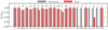 |
Fig. 3 Recovered atomic lines from our code, per element, relative to the list of the Gaia-ESO survey having synflag=‘Y’. The recovered lines for Arcturus and the Sun are plotted in grey and red, respectively. At the top of each bar, we report the number of lines identified in the Gaia-ESO survey for that element. |
4.2 Instrument design and optimisation
In this section, we investigate how such lines, selected in a similar way as in the previous section, compare for either a highresolution (R ~ 20 000) and a low-resolution (R ~ 6000) set-up. We once again took the case of the Sun and Arcturus, with the parameters defined in the previous section, as illustrative of a metal-rich turn-off star and a metal-poor giant.
Figures 5 and 6 show the lines that are selected for each set-up and each star, provided a minimum purity of 0.6 and a maximum S/Nresol = 50 for HR and S/Nresol = 100 for LR. A larger S/N threshold was adopted for LR, to mimic the fact that we would gain in terms of the S/N by going for LR mode at a fixed exposure time. We note that we assume that the S/N is the same across all of the wavelength range and that the wavelength range is the same for both set-ups. Neither of these assumptions are true, especially the first one, since noise is generally wavelength-dependent (e.g. wavelength dependent efficiency of spectrograph, decreasing optical quality at the borders of the detector, interstellar extinction absorbing preferentially in the blue, etc.).
For both the Sun and Arcturus, Figs. 5 and 6, show that the HR set-up contains a much wealthier selection of lines, for any of the considered elements. Indicatively, 233 (275) α-elements lines, 606 (769) Fe-peak lines, 10 (80) neutron-capture lines, and 26 (41) odd-Z elements lines were selected for the Sun (Arcturus) in HR, compared to 124 (78), 374 (375), 2 (8), and 11 (12) in LR, despite the higher S/N threshold (we recall, however, that the purity threshold is maintained equal to 0.6 in both cases). This corresponds to a “loss” of 50% to 90% of the lines (depending on the nucleosynthetic channel considered). In practice, going for LR implies giving up hopes of detection with a purity greater than 0.6 for Eu, Sm, Nd, Pr, Ce, Mo, Sr, Zn, and Cu for Arcturus, while for the Sun the problem is a bit less dramatic, losing only Y, Sr, and Zn (due to the fact that many of the aforementioned elements lost in Arcturus LR, are neither detected for the Sun in HR). Furthermore, the purity of the lines overall decreases when in LR, as expected due to the blending of the lines.
This application, illustrates which lines are detectable for specific spectral types, given a certain level of purity and the required S/Nresol, based on an instrumental resolving power. It can be used to choose wavelength ranges that contain the most information based on instrumental constraints (e.g. size of the CCD) or observational strategy (e.g. exposure time, target brightness, stellar type). In the following, we show how we use this information to assess which WEAVE-HR set-up performs best per nucleosynthetic channel and per element.
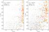 |
Fig. 4 Wavelength versus purity of the atomic lines selected over an arbitrary wavelength range for a Sun-like (left) and an Arcturus-like (right) spectrum at R = 20 000 (grey filled circles). The size of the points is proportional to the strength of the line, i.e. ~1 − coreflux. The subsample of the grey points that are selected as reliable lines for spectral synthesis from Heiter et al. (2021) for the Gaia-ESO survey (synflag=‘Y’) are highlighted in colour. Orange circles are associated to iron-peak lines, red to even-Z elements, blue to odd-Z elements and green to neutron-capture elements. We can see that the GES has selected lines that have, on average, a purity value greater than 0.8, with an overall greater purity for the Sun than for Arcturus. |
4.3 Choosing between set-ups: Application to the high-resolution set-ups of WEAVE
We now put ourselves in the framework of a survey design, such as WEAVE. There are two WEAVE Galactic archaeology (GA) HR surveys, a HR-chemodynamical survey targeting the thin and thick disc as well as the halo and an Open Cluster survey, aimed at targeting roughly a hundred young and old open clusters in the disc (Jin et al. 2023). WEAVE has the possibility to choose between two HR set-ups: the first one, dubbed in what follows as the B+R set-up, covers the wavelength ranges of [404–465] and [595–685] nm. The second one, dubbed G+R setup in what follows, covers the wavelength ranges of [473–545] and [595–685] nm. The question that we are trying to answer addresses which set-up combination probes the best the different nucleosynthetic channels. In other words, we consider which combination of set-ups maximises the number of elements and number of useful lines, per nucleosynthetic channel (α-elements, odd-Z elements, Fe-peak elements, neutron-capture elements) across the targeted parameter space of Teff, log g, and [M/H].
To set this value, we rely on WEAVE’s GA survey plan (WEAVE consortium, priv. comm.) and adopt as a threshold S/Nresol = 70, which is the value of the expected S/N peak in the blue set-up for the typical selection of the WEAVE GA-HR baseline survey. Other set-ups are expected to have a higher S/Nresol value. Using Eqs. (A.5) and (A.6), this corresponds to a minimum required depth of ~0.94 for a line to be detected.
We ran our code on a set of metal-poor stars ([M/H] = −2, representative of the halo), intermediate-metallicity stars ([M/H] = −0.5, representative of the thick disc), and metal-rich stars ([M/H] = 0, representative of the thin disc and open cluster stars). The results are shown in Figs. 7–9, for α-elements, Fe-peak elements and neutron-capture elements, respectively (we have not plotted the results for Teff = 4250 K and log g = 5.0 for visualisation purposes). They illustrate the number of lines (colour-code) and number of different elements (size of the points) detected for each nucleosynthetic family and each combination of Teff and log g. The purity threshold for the α-, Fe-peak, and neutron-capture elements has been arbitrarily set at 0.8, 0.9, and 0.6, in order to optimise the number of lines and the purity itself. A detailed view of the detected lines per element across the Kiel diagram is shown in the Appendix (see Figs C.1 to C.9).
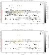 |
Fig. 5 Lines detected for a HR (R = 20 000, top) and a LR (R = 6000, bottom) set-up, for a Solar-like star. The names of the elements are indicated on the left-hand side of the plots. The number of identified lines is written in red, next to each element. The points are located at the wavelength where a line is detected. The area of the circles is proportional to the purity of the line, and their colour to the minimum S/Nresol required to detect the line. A simple way to read this plot is the following: if a point is difficult to visualise (small in size and white), then the spectral line is difficult to detect and use. The minimum purity plotted is 0.6. Similarly, lines that require a S/Nresol > 50 in HR or S/Nresol > 100 in LR are excluded. Indicatively, yellow ’+’ symbols are located to the wavelengths at which the Gaia-ESO survey has identified, for R = 40 000, lines that are reliable and pure for spectral synthesis (synflag=‘Y’, see Heiter et al. 2021, and Sect. 4.1). |
4.3.1 Even-Z elements
As shown in Fig. 7, the red set-up is the one clearly driving the science for intermediate and high metallicities, with more than ~30 useful lines throughout the Kiel diagram and four elements detected with a purity greater than 0.8 (the black solid circle in Fig. 7 is proportional to four elements). For metal-poor stars ([M/H] = −2), the blue set-up performs slightly better than the green and red set-ups, with more elements and more lines detected. The green set-up performs slightly better than the blue one for intermediate and high metallicities; this is known as a regime, however, where, as stated above, the red set-up is the one driving the science for α-elements. More specifically, based on Figs. C.1 and C.2, the following diagnostics can be drawn about individual elements:
Carbon (atomic) is seen both in green and red (but not for metal-poor stars) set-ups, with a purity a bit higher for the green set-up (p ≳0.7–0.8). It is not detectable in the blue set-up. We note, however, that these are high excitation C I lines, most readily visible in warmer stars, while C measurements may be achieved using molecular features such as CH in cooler stars.
Oxygen is only detectable in the red set-up via the λ = 630 nm line.
Magnesium is detectable in all three set-ups. The green setup has lines with a very good purity for every metallicity regime (thanks to the Mg I triplet). The blue set-up contains useful lines too, but with a lower purity (p ≲ 0.7).
Silicon has many lines detected in the red set-up (>20), as opposed to the green and blue set-ups which are not optimal for this element (less than 10 lines and p ≲ 0.7).
Sulphur is only detectable in the red set-up, for high- and intermediate-metallicity stars, with p ≳ 0.8.
Calcium has many detectable lines (more than four at each set-up) and its purity is very good in the red (p ≳ 0.9). The blue set-up performs better than the green, with more lines and higher purity.
Titanium has many lines detectable in all set-ups, with an overall low purity compared to other α-elements. For low-metallicity stars, the green set-up is preferred to the blue one, as it shows a higher purity.
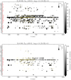 |
Fig. 6 Lines detected for a HR (R = 20 000, top) and a LR (R = 6000, bottom) set-up, for an Arcturus-like giant. See Fig. 5 for further details. |
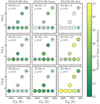 |
Fig. 7 Kiel-diagrams for stars with [Fe/H] = −2 (top), −0.5 (middle), 0.0 (bottom), and the three different WEAVE HR set-ups (blue: left, green: middle, and red: right). The colour code represents the number of lines associated with α-elements (O, Mg, Si, S, Ca, Ti) having a purity greater than 0.8 and detectable for a S/Nresoļ < 70. The size of the points is proportional to the number of α-elements with useful lines at a given combination of Teff, log g, and [M/H], As a reference, the size of a point for which four elements would have been detected is plotted as a black solid circle at the position of the Kiel diagram, for which we have templates. |
4.3.2 Odd-Z elements
No global plot combining the odd-Z elements is presented, as these cannot be linked to a specific nucleosynthetic channel. Nevertheless, their abundance determination is of prime importance on many fields of galactic and stellar evolution, and a thorough description on how the set-ups perform is necessary. Based on Figs. C.3 and C.4, the following diagnostics can be drawn:
Lithium is detected at all stellar types and metallicities in the red set-up, thanks to the λ = 670.8 nm line, and additionally at λ = 610.3 nm for the most metal-poor giant stars. We recall, however, that given the adopted Li abundance in the modelled spectra, A(Li) = 2.00 dex, our results are likely overestimated for giants (for which due to dilution A(Li) < 1; see, however, the case of Li-rich giants, e.g. Charbonnel & Balachandran 2000) and under-estimated for more metal-rich turn-off stars (see Karakas & Lattanzio 2014, and references therein).
Nitrogen (atomic) is not detectable in any of the set-ups.
Sodium is detected in the red set-up for all stars, except for the metal-poor regime, with p ≳ 0.75. The green and blue set-ups perform similarly, each of them providing low-purity lines (p ≲ 0.7) that do not allow for detections across the whole Kiel diagram at any metallicities.
Aluminium is seen only in the red, for intermediate and high metallicities. The purity is generally high (p ≳ 0.8).
Phosphorus is not detectable with either of the set-ups.
Potassium is not detectable in either of the set-ups.
Scandium is detected in the red set-up with p ≳ 0.85. Green and blue set-ups also contain useful Sc lines, especially at low metallicities, although with a lower purity than in the red set-up. The green set-up performs better than the blue one both in terms of number of lines and in terms of purity.
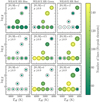 |
Fig. 8 Number of lines associated with iron-peak elements (V, Cr, Μn, Fe, Co, Ni, Cu, Zn) having a purity greater than 0.9 detectable for a S/Nresoļ < 70, at different regions of the Kiel diagram, for three metallicity regimes and WEAVE set-ups. See Fig. 7 for further details. |
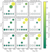 |
Fig. 9 Number of lines associated with neutron-capture elements (Rb, Sr, Y, Zr, Mo, Ba, La, Ce, Pr, Nd, Sm, Eu) having a purity greater than 0.6 detectable for a S/Nresoļ < 70, at different regions of the Kiel diagram, for three metallicity regimes and WEAVE set-ups. See Fig. 7 for further details. |
4.3.3 Fe-peak elements
As shown in Fig. 8, a plethora of lines is available for selection, with more than 60 lines characterised by a purity greater than 0.9 for any of the set-ups. Overall, the green set-up performs the best for all stars at low metallicity, as well for main-sequence stars at intermediate metallicity. The red set-up is the one driving the science for giants at intermediate metallicity and for all stars at high metallicity. The combination of the green and red set-ups allows us to get at least seven iron-peak elements at any combination of Teff, log g, and [M/H]. More specifically, based on Figs. C.5 and C.6, the following diagnostics can be drawn about individual elements:
Vanadium has high purity lines in the red set-up (p ≳ 0.8). The blue set-up performs better than red or green at low metallicity, with lines detected over the entire Kiel diagram.
Chromium has few high purity lines in the red set-up for intermediate and high metallicities. At low metallicity, both the green and blue set-ups exhibit many lines, with a marginal advantage of the green set-up over the blue one in terms of purer lines.
Manganese has the highest purity lines for intermediate and high metallicity stars in the red set-up, which also performs relatively well at low metallicity. Overall, the green set-up performs better than the blue, with the former having purer lines than the latter.
Iron has many lines that are detectable in all set-ups and, in fact, Fe I dominates the number counts in Fig. 8. The red setup has the highest purity (p ≳ 0.8) and the green set-up has purer Fe lines than the blue.
Cobalt has the purest lines in the red set-up. The blue set-up performs better than green at low metallicity, allowing for a detectability of Co lines for both giants and main sequence stars with a purity of 0.7–0.8.
Nickel has the purest lines in the red set-up. The green setup performs much better than the blue, with more numerous lines of greater purity.
Copper has lines seen only in the green, with a relatively low purity (p ≲ 0.7), except for metal-poor stars, where p ≳ 0.8.
Zinc is not seen in the blue set-up. The green set-up is the only one that allows us to measure a Zn abundance at low metallicities.
4.3.4 Neutron-capture elements
As shown in Fig. 9, WEAVE set-ups contain much less useful neutron-capture element lines than for the α- and Fe-peak elements, with (at best) 20 lines for metal-rich and intermediate metallicity giants. As far as the turn-off region is concerned, the blue set-up is shown to be performing the best, with more elements being probed compared to the other two set-ups.
More specifically, based on Figs. C.7–C.9, the following diagnostics can be drawn about individual elements:
Rubidium is never detected with a purity greater than 0.5 in the considered set-ups.
Strontium is detected only in the blue set-up (reaching p ≳ 0.8 for metal-poor stars).
Yttrium has a better purity in the green set-up compared to the blue. Yet, for intermediate and high metallicity stars, and Y lines are also detected in the red set-up.
Zirconium is best detected across the Kiel diagram in the green set-up and sparsely in the blue for main sequence and the red set-up for cool stars. However, the purity is overall low (p ≲ 0.7).
Molybdenum is detected only in the red set-up, only for the cooler and [Fe/H] > −0.5 dex stars, with p ≳ 0.7.
Barium is detected in all three set-ups, with the blue one performing slightly better than the green one in terms of purity.
Lanthanum is sparsely detected in all set-ups for giants with a variety of purities. There is a slight advantage of the green set-up over the blue, with purer and more numerous lines.
Cerium is detected at all evolutionary stages only the blue set-up, albeit with a low purity.
Praseodymium is sparsely detected in the blue and green set-ups.
Neodymium has the most numerous lines detected in the green set-up at any evolutionary stage, while having a similar purity similar than the other set-ups, at intermediate and high metallicities (or better in the case of metal-poor stars).
Samarium is slightly better detected in the blue set-up than in the other two set-ups.
Europium is only detected in the blue set-up for metal-poor stars, while only the red set-up allows the detection of usable lines for intermediate and high-metallicity giants. No lines are detected in the green set-up.
4.3.5 Summary
The diagnostics above were derived for an idealised case of perfectly normalised spectra with white noise (S/N values that are constant over the wavelength range). In reality, this will not be the case and the normalisation is expected to be challenging in the blue set-up, due to the multiple atomic and molecular lines. Yet, keeping in mind that WEAVE’s HR baseline survey will not target many cool main sequence stars (WEAVE consortium, priv. comm.), our results seem to slightly privilege the green+red set-up, both in numbers of elements detected and in terms of number of lines that are useful. We note, however, that there is a disparity in terms of which elements are detected over each of the set-ups (e.g. Sr is only detectable in the blue set-up) and that the final decision needs to be taken according to the elements that the science cases of the considered surveys decide to highlight and on the expected temperature and metallicity ranges in which those elements need to be detected (i.e. the target selection function).
4.4 Line-list optimisation for abundance determinations
For some abundance determination codes, the masking of a subset of lines of a specific element may be desired, either in order to decrease the computational time and/or to improve the precision of the measurement. The code presented in Sect. 2, allows us to very simply extract a sub-sample of lines for a given element, provided some observational (e.g. maximum S/N) and purity constraints. To build such a ‘golden line-sublisť, we could consider, for each given stellar type and metallicity, selecting lines that (i) maximise the purity; (ii) allow for an abundance measurement for both a high and a low S/N reflecting the range in apparent magnitudes of the survey; (iii) are preferably on the linear part of the curve-of-growth (i.e. not strong lines), to maximise the sensitivity of the lines to the elemental abundance (Gray 2005); (iv) span a wide range of excitation potentials to enable checks of the excitation temperature, or at least that do not have the lowest excitation potential values (typically more prone to non-local thermodynamic equilibrium); and (v) for which the synthetic lines satisfactorily reproduce the observed spectra of at least the Sun and Arcturus.
We implemented the above scheme into the creation of a line list for the blue HR set-up of WEAVE. In practice, we imposed S/Nresol,max = 70 as the maximum S/Nresol for the detectability of a line with no purity filter. For each element, we kept all of the available lines if their total number was less than 30 (this number was arbitrarily chosen) when considering all of the set of stellar atmospheric parameters. When there were more than 30 lines available, each stellar spectrum was investigated automatically, splitting the range of [0, S/Nresol,max] into three bins of equal range, and looking within each of these bins for the lines that had the highest purity. In order to achieve this, we started by imposing a purity of 1 and decreased the latter iteratively by steps of 0.025 until a minimum of five lines was reached while keeping the purity greater than 0.6 (except for Fe, where we imposed a minimum purity of 0.95). Figure 10 shows, for Ti, the properties of all the available lines detectable up to S/Nresol = 500, where we have highlighted in red the ones that we eventually select.
The golden line-sublist for the considered element was then obtained by keeping the union of all of the selected lines across the entire set of atmospheric parameters. Figure 11 shows a histogram of the excitation potential of all the available Ti lines detectable for S/Nresol,max (in grey) and in red, the sub-sample that we selected. We can see that they successfully span all the range of Eχ, with a bias towards lower values, as desired.
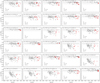 |
Fig. 10 Flux at the core of the lines versus purity of the lines for a given element (Ti) and different stellar types (parameters written at the top of each panel). The total available lines, from VALD, are in grey and the selected golden-subsample is in red. The dashed line is located at our S/Nresoļ threshold of 70, i.e. the lines need to be deeper than this in order to be detected. The other two dotted lines split the S/N range from 0 to 70 into three, within which we can select at least five lines, provided they have a purity greater than 0.6. |
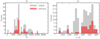 |
Fig. 11 Distribution of excitation potential (Eχ, left) and wavelengths (right) of all the Ti lines available in VALD (in grey) and the selected golden sub-sample (in red), the latter being the union of the lines selected in Fig. 10 for each stellar type. |
5 Conclusions
Our automatic line selection for abundance determination code is based on the use of synthetic spectra containing all of the elements and blends available and the comparison with a synthetic spectrum at the same stellar parameters containing only one element at the time. In this sense, a comparison with true, observed, spectra is necessary in order to confirm that the lines that are selected also represent the observed lines accurately. Ideally, this comparison should be done with spectra of stars for which both stellar parameters and individual abundances are best known, such as the Sun, Arcturus, and other benchmark stars (e.g. Blanco-Cuaresma et al. 2014; Heiter et al. 2015; Jofré et al. 2015). We have not proceeded with this comparison in this work, as results may vary from one resolving power to the other, yet a simple computation of residuals between the synthetic spectra and the real ones, around the lines that our code selects, should suffice to discard lines that are not modelled properly.
Our code can serve both as an illustration of where the chemical information is present in a stellar spectrum, but, most importantly, this allows us to optimise: i) observational strategies, such as choosing resolution and spectral windows, as well as ii) analysis codes, with the application of masks of high quality. In particular, direct applications for observations using the WEAVE (Jin et al. 2023) and 4MOST (de Jong et al. 2019) facilities (both community and consortium surveys) will benefit greatly from the tool presented here.
The Python code that allows us to identify and characterise useful lines can be downloaded on gitlab9. We also share via CDS the Tables containing the results at five different resolving powers (R = 3000, 6000, 20 000, 40 000 and 80 000) for lines that have a purity greater than 0.4 in at least one of their wings (i.e. pb or pr, see Sect. 2.1) for the entire wavelength range between 300 nm and 1000 nm. Results for other resolving powers can be easily computed and provided by contacting the first author of this paper. Finally, the 54 infinite resolution spectra that have been used in this work (~145 GB) can be shared upon request.
Acknowledgments
We thank the anonymous referee for their comments that helped improving the quality of the paper. This work has benefited from inspiring and fruitful discussions within the WEAVE and 4MOST consortia, as well as with Michael Hanke. Shoko Jin and Scott Trager are warmly thanked for their valuable feedback on early versions of the paper and for discussions that led to the selection of the WEAVE HR wavelength ranges. GK and VH gratefully acknowledge support from the french national research agency (ANR) funded project MWDisc (ANR-20-CE31-0004). KL acknowledges funds from the European Research Council (ERC) under the European Union’s Horizon 2020 research and innovation programme (Grant agreement no. 852977) and funds from the Knut & Alice Wallenberg foundation. This work was supported by the Programme National Cosmology et Galaxies (PNCG) of CNRS/INSU with INP and IN2P3, co-funded by CEA and CNES. Ansgar Wehrhahn is acknowledged for their contribution to the PySME code. This work has made use of the VALD database, operated at Uppsala University, the Institute of Astronomy RAS in Moscow, and the University of Vienna. as well as the Python packages Numpy (Harris et al. 2020), Matplotlib (Hunter 2007) and Pandas.
Appendix A Cayrel's formula and minimum depth of a line
Here, we derive our approximation on the desired minimum depth of a line, fmin, to be detected at a given S/N. We start from the standard Cayrel (1988) formula, linking the uncertainty σEW on measuring the equivalent width EW of a line, to the S/N per pixel, the full width at half-maximum of the line (assuming it has a Gaussian profile) and the pixel size, dx, (in wavelength units):
 (A.1)
(A.1)
To a good approximation, EW ≈ ƒmin · FWHM. We can therefore derive the formula for the uncertainty of the core of the line, σfmin, as:
 (A.2)
(A.2)
 (A.3)
(A.3)
where FWHM and dx are in wavelength units, and S/N is given per pixel.
Equation A.3 can also be expressed as a function of S/N per resolution element,  , as follows:
 (A.4)
(A.4)
 (A.5)
(A.5)
The detectability of a spectral absorption line is therefore possible if its intrinsic intensity is deeper than:
 (A.6)
(A.6)
Appendix B Equivalent width uncertainties in presence of a blend
We consider EW0 as the measured EW of a line, which we assume to be a combination of the real EW of the line alone, EWR, and a fractional contribution of a blend to the line, blend. We can thus write:
 (B.1)
(B.1)
The contribution of the blending to the error on EW0 can be written as:
 (B.2)
(B.2)
 (B.3)
(B.3)
 (B.4)
(B.4)
In order to have an error on EW0 smaller than 10% (corresponding to an abundance uncertainty of ~ 0.05 dex if the line is in the linear part of the curve of growth), we thus require:
 (B.5)
(B.5)
and, hence: 0.9 · blend ≤ 0.1 ⇒ blend ≤ 0.11.
Similarly, assuming that the blend is known by a factor of a, we can write:
 (B.6)
(B.6)
Following the previous steps, in order to have an error smaller than 10% on EW0, we therefore need:
 (B.7)
(B.7)
and hence: (a − 0.1) · blend ≤ 0.1 ⇒ blend  . So that if a = 0.5, then blend ≤ 0.25.
Appendix C Purities and detectability of elements for WEAVE high-resolution set-ups
The plots in this appendix represent the amount of lines detected per element and per combination of Teff-log g-[M/H] (size of the points) and the mean purity of the lines (colour-coded) at each point of the Kiel diagram, for each of WEAVE’s HR set-up. Figures are separated into even-Z (Fig. C.1 and C.2), odd-Z (Figs. C.3 and C.4), Fe-peak (Figs. C.5 and C.6), and neutron-capture elements (Figs. C.7, C.8 and C.9). The figures are discussed in Sect. 4.3.
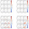 |
Fig. C.1 Number of identified lines (size of the points) and average purity (colour-coded) for the even-Z elements C, O, Mg, and Si, at different combinations of Teff, log g, and [Fe/H], for the different WEAVE HR set-ups. To guide the eye, black circles proportional to the identification of five lines are also plotted for each combination of Teff-log g (noting that the relative size of the black circles and, hence, of the coloured points change from one frame to the other, for visualisation purposes). The absence of coloured points implies the non-detection of lines. A minimum purity threshold of 0.5 has been set. The average ( |


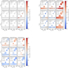 |
Fig. C.2 Number of identified lines (size of the points) and average purity (colour-coded) for the even-Z elements S, Ca, and Ti, at different combinations of Teff, log g, and [Fe/H], for the different WEAVE HR set-ups. See Fig. C.1 or further details. |
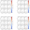 |
Fig. C.3 Number of identified lines (size of the points) and average purity (colour-coded) for the odd-Z elements Li, N, Na, and Al, at different combinations of Teff, log g, and [Fe/H], for the different WEAVE HR set-ups. See Fig. C.1 or further details. |
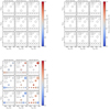 |
Fig. C.4 Number of identified lines (size of the points) and average purity (colour-coded) for the odd-Z elements P, K, and Sc, at different combinations of Teff, log g, and [Fe/H], for the different WEAVE HR set-ups. See Fig. C.1 or further details. |
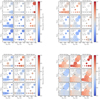 |
Fig. C.5 Number of identified lines (size of the points) and average purity (colour-coded) for the Fe-peak elements V, Cr, Mn, and Fe, at different combinations of Teff, log g, and [Fe/H], for the different WEAVE HR set-ups. See Fig. C.1 or further details. |
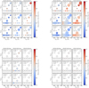 |
Fig. C.6 Number of identified lines (size of the points) and average purity (colour-coded) for the Fe-peak elements Co, Ni, Cu, and Zn, at different combinations of Teff, log g, and [Fe/H], for the different WEAVE HR set-ups. See Fig. C.1 or further details. |
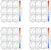 |
Fig. C.7 Number of identified lines (size of the points) and average purity (colour-coded) for the neutron-capture elements Rb, Sr, Y, and Zr, at different combinations of Teff, log g, and [Fe/H], for the different WEAVE HR set-ups. See Fig. C.1 or further details. |
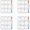 |
Fig. C.8 Number of identified lines (size of the points) and average purity (colour-coded) for the neutron-capture elements Mo, Ba, La, and Ce, at different combinations of Teff, log g, and [Fe/H], for the different WEAVE HR set-ups. See Fig. C.1 or further details. |
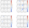 |
Fig. C.9 Number of identified lines (size of the points) and average purity (colour-coded) for the neutron-capture elements Pr, Nd, Sm, and Eu, at different combinations of Teff, log g, and [Fe/H], for the different WEAVE HR set-ups. See Fig. C.1 or further details. |
References
- Abareshi, B., Aguilar, J., Ahlen, S., et al. 2022, AJ, 164, 207 [NASA ADS] [CrossRef] [Google Scholar]
- Bedell, M., Meléndez, J., Bean, J. L., et al. 2014, ApJ, 795, 23 [Google Scholar]
- Blanco-Cuaresma, S., Soubiran, C., Jofré, P., & Heiter, U. 2014, A&A, 566, A98 [NASA ADS] [CrossRef] [EDP Sciences] [Google Scholar]
- Burbidge, E. M., Burbidge, G. R., Fowler, W. A., & Hoyle, F. 1957, Rev. Mod. Phys., 29, 547 [NASA ADS] [CrossRef] [Google Scholar]
- Caffau, E., Koch, A., Sbordone, L., et al. 2013, Astron. Nachr., 334, 197 [NASA ADS] [Google Scholar]
- Cayrel, R. 1988, in IAU Symposium, 132, The Impact of Very High S/N Spectroscopy on Stellar Physics, eds. G. Cayrel de Strobel, & M. Spite, 345 [CrossRef] [Google Scholar]
- Charbonnel, C., & Balachandran, S. C. 2000, A&A, 359, 563 [Google Scholar]
- Cirasuolo, M., Fairley, A., Rees, P., et al. 2020, The Messenger, 180, 10 [NASA ADS] [Google Scholar]
- Cropper, M., Katz, D., Sartoretti, P., et al. 2018, A&A, 616, A5 [NASA ADS] [CrossRef] [EDP Sciences] [Google Scholar]
- de Jong, R. S., Agertz, O., Berbel, A. A., et al. 2019, The Messenger, 175, 3 [NASA ADS] [Google Scholar]
- Deng, L.-C., Newberg, H. J., Liu, C., et al. 2012, Res. Astron. Astrophys., 12, 735 [Google Scholar]
- De Silva, G. M., Freeman, K. C., Bland-Hawthorn, J., et al. 2015, MNRAS, 449, 2604 [NASA ADS] [CrossRef] [Google Scholar]
- Feltzing, S. 2016, in Astronomical Society of the Pacific Conference Series, 507, Multi-Object Spectroscopy in the Next Decade: Big Questions, Large Surveys, and Wide Fields, eds. I. Skillen, M. Balcells, & S. Trager, 85 [Google Scholar]
- Freeman, K., & Bland-Hawthorn, J. 2002, ARA&A, 40, 487 [Google Scholar]
- Gaia Collaboration (Prusti, T., et al.) 2016, A&A, 595, A1 [NASA ADS] [CrossRef] [EDP Sciences] [Google Scholar]
- Gilmore, G., Randich, S., Worley, C. C., et al. 2022, A&A, 666, A120 [NASA ADS] [CrossRef] [EDP Sciences] [Google Scholar]
- Gray, D. F. 2005, The Observation and Analysis of Stellar Photospheres, 3rd edn. (Cambridge University Press) [Google Scholar]
- Grevesse, N., Asplund, M., & Sauval, A. J. 2007, Space Sci. Rev., 130, 105 [Google Scholar]
- Gustafsson, B., Edvardsson, B., Eriksson, K., et al. 2008, A&A, 486, 951 [NASA ADS] [CrossRef] [EDP Sciences] [Google Scholar]
- Hansen, C. J., Ludwig, H. G., Seifert, W., et al. 2015, Astron. Nachr., 336, 665 [NASA ADS] [CrossRef] [Google Scholar]
- Harris, C. R., Millman, K. J., van der Walt, S. J., et al. 2020, Nature, 585, 357 [NASA ADS] [CrossRef] [Google Scholar]
- Heiter, U., Jofré, P., Gustafsson, B., et al. 2015, A&A, 582, A49 [NASA ADS] [CrossRef] [EDP Sciences] [Google Scholar]
- Heiter, U., Lind, K., Bergemann, M., et al. 2021, A&A, 645, A106 [EDP Sciences] [Google Scholar]
- Hunter, J. D. 2007, Comput. Sci. Eng., 9, 90 [NASA ADS] [CrossRef] [Google Scholar]
- Iwamoto, K., Brachwitz, F., Nomoto, K., et al. 1999, ApJS, 125, 439 [NASA ADS] [CrossRef] [Google Scholar]
- Jin, S., Trager, S. C., Dalton, G. B., et al. 2023, MNRAS, in press, https://doi.org/10.1093/mnras/stad557 [Google Scholar]
- Jofré, P., Heiter, U., Soubiran, C., et al. 2015, A&A, 582, A81 [Google Scholar]
- Jofré, P., Heiter, U., & Soubiran, C. 2019, ARA&A, 57, 571 [Google Scholar]
- Karakas, A. I., & Lattanzio, J. C. 2014, PASA, 31, e030 [NASA ADS] [CrossRef] [Google Scholar]
- Kordopatis, G., Recio-Blanco, A., de Laverny, P., et al. 2011, A&A, 535, A106 [NASA ADS] [CrossRef] [EDP Sciences] [Google Scholar]
- Kordopatis, G., Gilmore, G., Steinmetz, M., et al. 2013, AJ, 146, 134 [Google Scholar]
- Kordopatis, G., Schultheis, M., McMillan, P. J., et al. 2023, A&A, 669, A104 [NASA ADS] [CrossRef] [EDP Sciences] [Google Scholar]
- Majewski, S. R., Schiavon, R. P., Frinchaboy, P. M., et al. 2017, AJ, 154, 94 [NASA ADS] [CrossRef] [Google Scholar]
- Ness, M., Hogg, D. W., Rix, H. W., Ho, A. Y. Q., & Zasowski, G. 2015, ApJ, 808, 16 [NASA ADS] [CrossRef] [Google Scholar]
- Nomoto, K., Kobayashi, C., & Tominaga, N. 2013, ARA&A, 51, 457 [CrossRef] [Google Scholar]
- Piskunov, N., & Valenti, J. A. 2017, A&A, 597, A16 [NASA ADS] [CrossRef] [EDP Sciences] [Google Scholar]
- Piskunov, N. E., Kupka, F., Ryabchikova, T. A., Weiss, W. W., & Jeffery, C. S. 1995, A&As, 112, 525 [Google Scholar]
- Randich, S., Gilmore, G., Magrini, L., et al. 2022, A&A, 666, A121 [NASA ADS] [CrossRef] [EDP Sciences] [Google Scholar]
- Recio-Blanco, A., Bijaoui, A., & de Laverny, P. 2006, MNRAS, 370, 141 [Google Scholar]
- Ruchti, G. R., Feltzing, S., Lind, K., et al. 2016, MNRAS, 461, 2174 [NASA ADS] [CrossRef] [Google Scholar]
- Ryabchikova, T., Piskunov, N., Kurucz, R. L., et al. 2015, Phys. Scr, 90, 054005 [Google Scholar]
- Sandford, N. R., Weisz, D. R., & Ting, Y.-S. 2020, ApJS, 249, 24 [NASA ADS] [CrossRef] [Google Scholar]
- Sheinis, A., Anguiano, B., Asplund, M., et al. 2015, J. Astron. Telescopes Instrum. Syst., 1, 035002 [NASA ADS] [CrossRef] [Google Scholar]
- Smiljanic, R., Korn, A. J., Bergemann, M., et al. 2014, A&A, 570, A122 [NASA ADS] [CrossRef] [EDP Sciences] [Google Scholar]
- Takada, M., Ellis, R. S., Chiba, M., et al. 2014, PASJ, 66, R1 [Google Scholar]
- The MSE Science Team (Babusiaux, C., et al.) 2019, arXiv e-prints, [ArXiv:1904.04907] [Google Scholar]
- Ting, Y.-S., Conroy, C., Rix, H.-W., & Cargile, P. 2017, ApJ, 843, 32 [NASA ADS] [CrossRef] [Google Scholar]
- Valenti, J. A., & Piskunov, N. 1996, A&AS, 118, 595 [NASA ADS] [CrossRef] [EDP Sciences] [Google Scholar]
- Wehrhahn, A., Piskunov, N., & Ryabchikova, T. 2023, A&A, 671, A171 [NASA ADS] [CrossRef] [EDP Sciences] [Google Scholar]
- Zhao, G., Zhao, Y.-H., Chu, Y.-Q., Jing, Y.-P., & Deng, L.-C. 2012, Res. Astron. Astrophys., 12, 723 [NASA ADS] [CrossRef] [Google Scholar]
Retrieved from the Vienna Atomic Line Database (VALD), http://vald.astro.uu.se/
We note that in doing so, we assume that all of the lines are at the same ionisation level, which is not necessarily the case, unless S Ε(λ) is computed only for a given ionisation level.
Several ionisation levels can be present in the element spectrum in case the user does not wish to differentiate between them.
Assuming that no rapid-rotators are to be observed and that macroturbulence does not dominate the line-profile.
We do not consider, for this work, the hydrogen lines. We kept only one line per element if within 0.01 nm from the others.
The cross-match was performed by rounding the wavelength to 0.01 nm.
All Tables
Non-exhaustive list of spectrographs used for galactic archaeology covering the optical wavelengths at different resolving powers.
All Figures
|
Fig. 1 Examples of identified lines for a Solar-like spectrum at R = 20 000. The elemental spectrum, i.e. the flux computed with the contribution from atomic lines from only one ionization stage of one element, is plotted in red. The full spectrum containing all of the elements and molecules is shown in black. The element and ionization stage associated to the line are noted on the upper left corner of each plot. The central wavelength of the identified line, λc is plotted as a vertical dashed grey line. The blue-end and the red-end of the line are plotted as vertical dashed green lines. The depth of the line in the element spectrum is indicated at the bottom left corner of each plot. The purity factor for the entire line is written at the middle-top of the plots. The blue-wing and red-wing purities are enclosed within the line at its left and right, respectively. |
| In the text | |
|
Fig. 2 Set of atmospheric parameters for which the full and elemental synthetic spectra were computed. |
| In the text | |
|
Fig. 3 Recovered atomic lines from our code, per element, relative to the list of the Gaia-ESO survey having synflag=‘Y’. The recovered lines for Arcturus and the Sun are plotted in grey and red, respectively. At the top of each bar, we report the number of lines identified in the Gaia-ESO survey for that element. |
| In the text | |
|
Fig. 4 Wavelength versus purity of the atomic lines selected over an arbitrary wavelength range for a Sun-like (left) and an Arcturus-like (right) spectrum at R = 20 000 (grey filled circles). The size of the points is proportional to the strength of the line, i.e. ~1 − coreflux. The subsample of the grey points that are selected as reliable lines for spectral synthesis from Heiter et al. (2021) for the Gaia-ESO survey (synflag=‘Y’) are highlighted in colour. Orange circles are associated to iron-peak lines, red to even-Z elements, blue to odd-Z elements and green to neutron-capture elements. We can see that the GES has selected lines that have, on average, a purity value greater than 0.8, with an overall greater purity for the Sun than for Arcturus. |
| In the text | |
|
Fig. 5 Lines detected for a HR (R = 20 000, top) and a LR (R = 6000, bottom) set-up, for a Solar-like star. The names of the elements are indicated on the left-hand side of the plots. The number of identified lines is written in red, next to each element. The points are located at the wavelength where a line is detected. The area of the circles is proportional to the purity of the line, and their colour to the minimum S/Nresol required to detect the line. A simple way to read this plot is the following: if a point is difficult to visualise (small in size and white), then the spectral line is difficult to detect and use. The minimum purity plotted is 0.6. Similarly, lines that require a S/Nresol > 50 in HR or S/Nresol > 100 in LR are excluded. Indicatively, yellow ’+’ symbols are located to the wavelengths at which the Gaia-ESO survey has identified, for R = 40 000, lines that are reliable and pure for spectral synthesis (synflag=‘Y’, see Heiter et al. 2021, and Sect. 4.1). |
| In the text | |
|
Fig. 6 Lines detected for a HR (R = 20 000, top) and a LR (R = 6000, bottom) set-up, for an Arcturus-like giant. See Fig. 5 for further details. |
| In the text | |
|
Fig. 7 Kiel-diagrams for stars with [Fe/H] = −2 (top), −0.5 (middle), 0.0 (bottom), and the three different WEAVE HR set-ups (blue: left, green: middle, and red: right). The colour code represents the number of lines associated with α-elements (O, Mg, Si, S, Ca, Ti) having a purity greater than 0.8 and detectable for a S/Nresoļ < 70. The size of the points is proportional to the number of α-elements with useful lines at a given combination of Teff, log g, and [M/H], As a reference, the size of a point for which four elements would have been detected is plotted as a black solid circle at the position of the Kiel diagram, for which we have templates. |
| In the text | |
|
Fig. 8 Number of lines associated with iron-peak elements (V, Cr, Μn, Fe, Co, Ni, Cu, Zn) having a purity greater than 0.9 detectable for a S/Nresoļ < 70, at different regions of the Kiel diagram, for three metallicity regimes and WEAVE set-ups. See Fig. 7 for further details. |
| In the text | |
|
Fig. 9 Number of lines associated with neutron-capture elements (Rb, Sr, Y, Zr, Mo, Ba, La, Ce, Pr, Nd, Sm, Eu) having a purity greater than 0.6 detectable for a S/Nresoļ < 70, at different regions of the Kiel diagram, for three metallicity regimes and WEAVE set-ups. See Fig. 7 for further details. |
| In the text | |
|
Fig. 10 Flux at the core of the lines versus purity of the lines for a given element (Ti) and different stellar types (parameters written at the top of each panel). The total available lines, from VALD, are in grey and the selected golden-subsample is in red. The dashed line is located at our S/Nresoļ threshold of 70, i.e. the lines need to be deeper than this in order to be detected. The other two dotted lines split the S/N range from 0 to 70 into three, within which we can select at least five lines, provided they have a purity greater than 0.6. |
| In the text | |
|
Fig. 11 Distribution of excitation potential (Eχ, left) and wavelengths (right) of all the Ti lines available in VALD (in grey) and the selected golden sub-sample (in red), the latter being the union of the lines selected in Fig. 10 for each stellar type. |
| In the text | |
|
Fig. C.1 Number of identified lines (size of the points) and average purity (colour-coded) for the even-Z elements C, O, Mg, and Si, at different combinations of Teff, log g, and [Fe/H], for the different WEAVE HR set-ups. To guide the eye, black circles proportional to the identification of five lines are also plotted for each combination of Teff-log g (noting that the relative size of the black circles and, hence, of the coloured points change from one frame to the other, for visualisation purposes). The absence of coloured points implies the non-detection of lines. A minimum purity threshold of 0.5 has been set. The average ( |
| In the text | |
|
Fig. C.2 Number of identified lines (size of the points) and average purity (colour-coded) for the even-Z elements S, Ca, and Ti, at different combinations of Teff, log g, and [Fe/H], for the different WEAVE HR set-ups. See Fig. C.1 or further details. |
| In the text | |
|
Fig. C.3 Number of identified lines (size of the points) and average purity (colour-coded) for the odd-Z elements Li, N, Na, and Al, at different combinations of Teff, log g, and [Fe/H], for the different WEAVE HR set-ups. See Fig. C.1 or further details. |
| In the text | |
|
Fig. C.4 Number of identified lines (size of the points) and average purity (colour-coded) for the odd-Z elements P, K, and Sc, at different combinations of Teff, log g, and [Fe/H], for the different WEAVE HR set-ups. See Fig. C.1 or further details. |
| In the text | |
|
Fig. C.5 Number of identified lines (size of the points) and average purity (colour-coded) for the Fe-peak elements V, Cr, Mn, and Fe, at different combinations of Teff, log g, and [Fe/H], for the different WEAVE HR set-ups. See Fig. C.1 or further details. |
| In the text | |
|
Fig. C.6 Number of identified lines (size of the points) and average purity (colour-coded) for the Fe-peak elements Co, Ni, Cu, and Zn, at different combinations of Teff, log g, and [Fe/H], for the different WEAVE HR set-ups. See Fig. C.1 or further details. |
| In the text | |
|
Fig. C.7 Number of identified lines (size of the points) and average purity (colour-coded) for the neutron-capture elements Rb, Sr, Y, and Zr, at different combinations of Teff, log g, and [Fe/H], for the different WEAVE HR set-ups. See Fig. C.1 or further details. |
| In the text | |
|
Fig. C.8 Number of identified lines (size of the points) and average purity (colour-coded) for the neutron-capture elements Mo, Ba, La, and Ce, at different combinations of Teff, log g, and [Fe/H], for the different WEAVE HR set-ups. See Fig. C.1 or further details. |
| In the text | |
|
Fig. C.9 Number of identified lines (size of the points) and average purity (colour-coded) for the neutron-capture elements Pr, Nd, Sm, and Eu, at different combinations of Teff, log g, and [Fe/H], for the different WEAVE HR set-ups. See Fig. C.1 or further details. |
| In the text | |
Current usage metrics show cumulative count of Article Views (full-text article views including HTML views, PDF and ePub downloads, according to the available data) and Abstracts Views on Vision4Press platform.
Data correspond to usage on the plateform after 2015. The current usage metrics is available 48-96 hours after online publication and is updated daily on week days.
Initial download of the metrics may take a while.