| Issue |
A&A
Volume 674, June 2023
|
|
|---|---|---|
| Article Number | A142 | |
| Number of page(s) | 11 | |
| Section | The Sun and the Heliosphere | |
| DOI | https://doi.org/10.1051/0004-6361/202245373 | |
| Published online | 15 June 2023 | |
Five-minute oscillations of photospheric and chromospheric swirls
1
Deep Space Exploration Laboratory/School of Earth and Space Sciences, University of Science and Technology of China, Hefei, 230026
PR China
e-mail: This email address is being protected from spambots. You need JavaScript enabled to view it.
2
Astrophysics Research Centre, School of Mathematics and Physics, Queen’s University Belfast, Belfast, BT7 1NN
UK
3
CAS Key Laboratory of Geospace Environment, Department of Geophysics and Planetary Sciences, University of Science and Technology of China, Hefei, 230026
PR China
4
Department of Physics and Astronomy, California State University Northridge, 18111 Nordhoff Street, Northridge, CA, 91330
USA
5
Solar Physics and Space Plasma Research Centre (SP2RC), School of Mathematics and Statistics, University of Sheffield, Hicks Building, Hounsfield Road, Sheffield, S3 7RH
UK
6
Department of Astronomy, Eötvös Loránd University, Pázmány P. sétány 1/A, Budapest, 1117
Hungary
7
Gyula Bay Zoltán Solar Observatory (GSO), Hungarian Solar Physics Foundation (HSPF), Petőfi tér 3., Gyula, 5700
Hungary
Received:
4
November
2022
Accepted:
12
April
2023
Abstract
Context. Swirls are ubiquitous in the solar atmosphere. They are thought to be related to the excitation of different modes of magnetohydrodynamic waves and pulses, as well as spicules. However, statistical studies of their collective behaviour are rare.
Aims. We aim to study the collective as well as the individual behaviour of photospheric and chromospheric swirls detected by the automated swirl detection algorithm (ASDA) from observations obtained by the Swedish 1-m Solar Telescope and the Hinode satellite.
Methods. We performed a detailed analysis of six different parameters of photospheric and chromospheric swirls with the wavelet analysis. Two clusters with periods with significant wavelet power, one from 3 − 8 min and the other from 10 − 14 min, were found. The former coincides with the dominant period of the global p-mode spectrum. The wavelet and fast Fourier transform analysis of example swirls also revealed similar periods.
Results. These results suggest that global p-modes might be important in triggering photospheric and thus chromospheric swirls. A novel scenario of global p-modes providing energy and mass fluxes to the upper solar atmosphere via generating swirls, Alfvén pulses, and spicules is then proposed.
Key words: Sun: photosphere / Sun: chromosphere / Sun: oscillations
© The Authors 2023
 Open Access article, published by EDP Sciences, under the terms of the Creative Commons Attribution License (https://creativecommons.org/licenses/by/4.0), which permits unrestricted use, distribution, and reproduction in any medium, provided the original work is properly cited.
This article is published in open access under the Subscribe to Open model. This email address is being protected from spambots. You need JavaScript enabled to view it. to support open access publication.
1. Introduction
Swirls are widely observed in different layers of the solar atmosphere (e.g. Wang et al. 1995; Bonet et al. 2008, 2010; Attie et al. 2009; Balmaceda et al. 2010; Wedemeyer-Böhm & Rouppe van derVoort 2009; Wedemeyer-Böhm et al. 2012; Su et al. 2014; Kato & Wedemeyer 2017; Liu et al. 2019a,b; Shetye et al. 2019). In addition to their ubiquity, they have been suggested to be related to a number of different magnetohydrodynamic (MHD) processes from the photosphere to the corona, including MHD waves and pulses (e.g. Carlsson et al. 2009; Fedun et al. 2011; Shelyag et al. 2013; Shukla 2013; Mumford & Erdélyi 2015; Leonard et al. 2018; Murawski et al. 2018; Kohutova et al. 2020; Battaglia et al. 2021), spicules or jets (e.g. Kitiashvili et al. 2012, 2013; Liu et al. 2019b; Oxley et al. 2020; Scalisi et al. 2021a,b; Bate et al. 2022; Dey & Chatterjee 2022), and (magnetic) bright points or magnetic concentrations (e.g. Balmaceda et al. 2010; Jess et al. 2010; Liu et al. 2019c; Shetye et al. 2019; Murabito et al. 2020). Further observations and numerical simulations suggest that swirls might be able to channel enough energy from the lower to the upper solar atmosphere (e.g. Wedemeyer-Böhm & Rouppe van der Voort 2009; Liu et al. 2019b; Yadav et al. 2021; Battaglia et al. 2021).
Detailed studies of individual swirls or a small collection of swirls have shown intriguing and important properties. For example, Wedemeyer-Böhm & Rouppe van der Voort (2009) analysed ten clear small-scale swirling candidates observed in the chromosphere by the Swedish 1-m Solar Telescope (SST; Scharmer et al. 2003) and found that these swirls could be related to the so-called magnetic tornadoes channelling energy into the solar corona. A series of investigations were conducted to establish the properties of a persistent quiet-Sun swirl whose lifetime exceeded 1.7 h (Tziotziou et al. 2018, 2019, 2020), including its associated waves and oscillations. However, owing to their ubiquity (> 105 swirls in the photosphere at any time; e.g. Liu et al. 2019a) and small scale (with an average radius of several hundred kilometres), statistical studies of manually selected swirls have proven difficult and may introduce undesired human bias. Several automated detection methods have recently been developed. Kato & Wedemeyer (2017) presented two detection algorithms that are based on a line integral convolution (LIC) imaging technique. One technique uses enhanced vorticity and the other the vorticity strength to identify swirls. Their methods were tested on a simulated chromosphere generated by the CO5BOLD (Freytag et al. 2012) numerical MHD code. Another method, recently proposed by Dakanalis et al. (2021), employs a series of processes including image pre-processing, tracing of curved structures, segmentation, and clustering. The last two processes are widely used in machine-learning techniques. This method was tested with synthetic data and observations obtained by the SST and was further suggested to be applicable for quasi-linear fibrillar structure detections following some modifications.
Employing the velocity field information estimated from successive images by Fourier local correlation tracking (FLCT; Welsch et al. 2004; Fisher & Welsch 2008), Liu et al. (2019a) developed an automated swirl detection algorithm (ASDA1). ASDA was applied to photospheric and chromospheric observations (Liu et al. 2019a,b) acquired by the Solar Optical Telescope (SOT; Tsuneta et al. 2008) on board Hinode (Kosugi et al. 2007) and by the CRisp Imaging SpectroPolarimeter (CRISP; Scharmer 2006) on the SST (Scharmer et al. 2003). A total number of more than 105 swirls were found in the photosphere at any moment of time, with an average radius of ∼300 km, a rotating speed of ∼1 km s−1, and a lifetime of about 20 s. Correlation analyses between photospheric and chromospheric swirls, together with three-dimensional MHD numerical simulations, suggested that ubiquitous Alfvén pulses might be excited by photospheric swirls and travel to the chromosphere (Liu et al. 2019b). The co-existence of intensity swirls and magnetic swirls (Liu et al. 2019c) in the simulated photosphere generated by the Bifrost code (Gudiksen et al. 2011; Carlsson et al. 2016) suggested that the necessary condition for the generation of Alfvén pulses in the solar atmosphere might be fulfilled. This scenario was confirmed by the MHD numerical simulation using the radiative MHD code CO5BOLD (Battaglia et al. 2021). Recent advances in analytical and numerical simulations (Oxley et al. 2020; Scalisi et al. 2021a,b; Singh et al. 2022) suggest that these Alfvén pulses might further drive mass motions upward, such as spicules, that propagate in the upper solar atmosphere.
In addition to these recent advances in observations, numerical simulations and theories of solar atmospheric swirls, we are not aware of many works that have studied the collective behaviours of swirls and their relation with global phenomena of the Sun, such as the five-minute global acoustic oscillations and the solar activity cycle. In this paper, we present evidence of the five-minute oscillation of photospheric and chromospheric swirls. This paper is organised as follows: Data and methods are briefly introduced in Sect. 2 before we present our results in Sect. 3 and draw the conclusions in Sect. 4.
2. Data and methods
Five sets of data are used in this study. The first three sets of data consist of wide-band photospheric images at Fe I 630.25 nm, chromospheric images at the Hα line core with a central wavelength of 656.3 nm, and chromospheric images at the Ca II line core with a central wavelength of 854.2 nm by SST/CRISP (Scharmer et al. 2003, 2008; Scharmer 2006) between 08:07:22 UT and 09:05:44 UT on 21 June 2012. The target was a quite-Sun region close to the disk centre (xc = −3″, yc = 70″) with a field of view (FOV) of 55″ × 55″. The spatial and temporal resolutions are 0.1″ and 8.25 s, respectively. The black and white background in Fig. 1a depicts an example of the SST chromospheric images at the Hα line core.
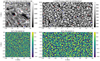 |
Fig. 1. Examples of swirls detected in SST and Hinode observations. the black and white backgrounds in panels a and c are the SST Hα line core chromospheric and SOT FG blue photospheric observations on 21 June 2012 and 5 March 2007, respectively. Red and blue contours are swirls detected by ASDA (Liu et al. 2019a) with clockwise and counter-clockwise rotations, respectively. Panels b and d are the Γ2 maps, corresponding to observations in panels a and c. Γ2 values are used to define edges of swirls (see e.g. Graftieaux et al. 2001; Liu et al. 2019a). Figure axes represent physical distances across the surface of the Sun (in Mm), with the origin of the chosen domain placed at the centre of the observing FOV. |
The other two sets of data consist of blue continuum (FG Blue) photospheric images with a central wavelength of 450.45 nm, and images at the Ca II H line with a central wavelength of 396.85 nm taken by Hinode/SOT (Kosugi et al. 2007; Tsuneta et al. 2008) between 05:48:03 UT and 08:29:59 UT on 5 March 2007. Each of them contains 1515 images of a quiet-Sun region close to the disk centre (xc = 5.3″, yc = 4.1″) with a FOV of ∼56″ × 28″. The spatial and temporal resolutions are 0.1″ and 6.42 s, respectively. Figure 1c depicts an example of the SOT FG blue photospheric images. We note that the broadband Ca II H observations by Hinode/SOT cover a wide range of altitudes from the photosphere to the chromosphere (Rutten et al. 2004; Carlsson et al. 2007).
ASDA (Liu et al. 2019a) was applied to every two successive images in each data set. ASDA contains two essential steps to perform the detection of swirls: (1) velocity field estimation using FLCT (Welsch et al. 2004; Fisher & Welsch 2008), and (2) vortex identification using two parameters (Γ1 and Γ2) proposed by Graftieaux et al. (2001). For each point in the velocity field, 49 points around it are used to calculate Γ1 and Γ2 to identify the centres and edges of swirls, respectively. A detailed description of ASDA and how the parameters including location, radius, rotating speed, expanding/shrinking speed, and lifetime of swirls are extracted from the Γ1 and Γ2 values was given in Liu et al. (2019a). In summary, Γ2 is used to identify swirl candidates and the regions they cover, while Γ1 is used to quantify the swirl strength. The red and blue curves in Figs. 1a,c are swirls that were detected by ASDA from the example SST Hα chromospheric observation and SOT FG blue photospheric observation, with clockwise rotations (red) and counter-clockwise rotations (blue), respectively. Figures 1b,d show the distributions of the Γ2 values calculated from the example observations. Figure 2 depicts examples of individual swirls detected using ASDA from SST and Hinode/SOT observations. Rows 2–6 display zoomed-in views of the dashed orange boxes in the first row. The panels in the second row show images and velocity fields ∼5 min before the example swirls, with curved streamlines at locations similar to where the swirls will form, indicating their prerequisites. The third to the sixth rows are the first, middle, and last frames of the example swirls, respectively. Consistent with the statistical findings in Liu et al. (2019a,c), these swirls are located at intergranular lanes (dark features in the first, third, fourth, and fifth columns). The last row shows the photospheric and chromospheric conditions ∼5 min after the example swirls.
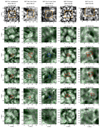 |
Fig. 2. Examples of individual swirls in SST and Hinode observations. The black and white backgrounds are the corresponding intensities at each passband. Rows 2–6 are the zoom-in views of the orange boxes in the first row. Green arrows are velocity fields estimated using FLCT. The red and blue curves are the edges of the example swirls with clockwise and counter-clockwise rotations, respectively (see main text for details). |
To explore the relation between photospheric and chromospheric swirls, bypassing a number of difficulties such as selection effects, the inclined magnetic field from the photosphere to the chromosphere, and the irregular shape of swirls, Liu et al. (2019b) proposed a new method for calculating the correlation coefficient between photospheric and chromospheric swirls. To quantify the collective behaviour of swirls in the same data set (i.e. the same layer in the solar atmosphere), we have adapted the above method, as follows:
– For the Γ2 maps of all images in a given layer, set all points to be 0 except those greater (less) than 2/π (−2/π), which are set to be 1 (−1).
– Take the first Γ2 map from the above as the reference and mark it as Γt1. Define T1 as the sum of the absolute values of all points in Γt1.
– Take the second Γ2 map and mark it as Γt2. Define T2 as the sum of the absolute values of all points in Γt2.
– Multiply Γt1 and Γt2 point by point to obtain the correlation map C. Their correlation coefficient CC is then defined as (∑C)/T, where T = max(T1, T2).
– Repeat the above processes for the rest frames to obtain their correlation coefficients with the first frame of the data set.
The definition of CC shows that it evaluates the similarity of the swirl distribution between two frames. This process is shown in Fig. 3.
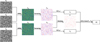 |
Fig. 3. Flowchart of how the correlation coefficient (CC) is calculated. It1, It2, and It3 are three frames of the intensity observations. Two Γ2 maps (Γt1 and Γt2) are generated from these three intensity observations employing ASDA (Liu et al. 2019a). They are further ternarised to contain only values of −1, 0, and 1. These ternarised Γ2 maps are then used to calculate CC. For more information, see the text provided in Sect. 2. |
3. Results
3.1. Overall parameters
Figure 4a depicts the distribution of CC for SST Hα line core chromospheric swirls. The correlation between each frame and the first frame drops quickly. The inset in panel a shows a zoomed-in view of the region before the dashed green line. The dashed blue line corresponds to a CC of 0.1 at ∼25 s. This is consistent with the average lifetime of photospheric and chromospheric swirls found using a different method (∼16 − 23 s, Liu et al. 2019a,b), and it again confirms the short-lived characteristics of these small-scale structures.
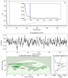 |
Fig. 4. Variation in CC and its wavelet power spectrum. Panel a is the distribution of CC vs. time for the SST Hα line core chromospheric swirls. See Sect. 2 for the definition of the CC. The inset in panel a is a zoomed-in view of the region before the dashed green line. The dashed blue line corresponds to a CC of 0.1. Panel b shows the variation in CC after applying a highpass filter and subtracting its average value. Panel c is the corresponding wavelet power spectrum with darker colours for higher powers. The solid black curves are the local 95% confidence levels. The solid black curve in panel d is the global wavelet power. Purple text indicates peaks above the 95% confidence level (dashed black line). The dotted black lines are used to determine the extension of each peak. |
We employed a wavelet analysis (Torrence & Compo 1998) to explore any potential periodicities in CC. To avoid the influence of the first few frames, which have a high correlation with the first frame, all frames before the dashed green line in Fig. 4a were omitted. Normally, an overall trend needs to be removed from the original time series to remove the undesired periods introduced by the long-term variation. This overall trend is usually generated as the rolling average with a certain window width of the original time series. However, this needs very careful consideration because false periods with values close to the window width can be introduced and thus contaminate the wavelet power spectrum.
Instead of subtracting the rolling average, we removed the long-term trend of the time series by applying a high-pass filter to it that greatly weakens all signals with a period longer than one-quarter of the length of the original time series. This approach is preferred as it does not introduce any false periods. The processed time series was then used for the wavelet analysis after subtracting its average value. Figure 4b shows the processed CC. Its wavelet power spectrum is shown in Fig. 4c with darker colours depicting stronger powers and black curves depicting 95% confidence levels. Several periods from 2 min to 8 min are found.
These periods are more obvious in the global wavelet spectrum (Fig. 4d). Two significant peaks at 2.7 min and 5.5 min are found above the 95% confidence level (dashed black curve in Fig. 4d). Horizontal dotted lines are used to estimate the extension of each peak. For a given peak, its extension is defined by the distance between the local minima or the local 95% confidence levels (whichever is closer to the target peak) on either side. The periods found by the wavelet analysis on the CC values of swirls in the SST Hα line core observations were then determined as 2.7 ± 1.5 min and 5.5 ± 1.8 min. Similar approaches using the wavelet analysis were applied to other properties of SST Hα line core chromospheric swirls, including the total number of swirls in each frame (N), their average intensity( ), average radius (
 ), average rotating speed (
 ), and average absolute expanding/shrinking speed (
 ). Similar periods from 2 min to 13 min are found, which are shown as the fourth row in Table 1. Any periods longer than one-quarter of the length of the time series are crossed out in the table.
Periods in units of minutes found from the wavelet analysis of the overall parameters of SOT and SST photospheric and chromospheric swirls.
Figure 5a shows the variation in the average intensity of SST Fe I wide-band photospheric swirls after the highpass filter was applied and its average value was subtracted. Figures 5b,c are the wavelet power spectrum and the global wavelet power, respectively. Only one significant period at 6.7 ± 1.1 min above the 95% confidence level was found. The periods found from the time series of other parameters of the SST photospheric swirls range from 2 min to 13 min (second row in Table 1). The remainder of Table 1 shows significant periods for the six parameters (CC, N,  ,
,  ,
,  , and
, and  ) of swirls detected in the SOT FG blue, SOT Ca II H, and SST Ca II line core. Eighty-four significant periods were found from all the 30 time series ranging from 1 min to 17 min, with an average value of 6.9 ± 4.4 min. Out of all 84 periods, 45 (∼54%) are between 2 min to 9 min.
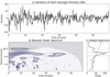 |
Fig. 5. Variation in the average intensity of swirls and its wavelet spectrum. Panels a–c are similar to panels b–d in Fig. 4, but for the SST Fe I 6302 wide-band photospheric swirls. |
3.2. Periodicity of individual swirls
To examine whether these periodicities also exist in individual swirls, we further applied the wavelet analysis and fast Fourier transformation (FFT) to the Γ1 and Γ2 maps in small regions centred on the example swirls shown in Fig. 2. To conduct the FFT analysis, cogitating on the example swirl in the SOT Ca II H observations (Fig. 2e), a three-dimensional data cube (x, y, t) 18 × 18 pix2 around the centre of the swirl was extracted from its Γ2 maps. 18 × 18 pix2 is about twice of the average diameter of swirls detected, and it was chosen to avoid mixing signals of multiple swirls in the FOV. This data cube was then converted from the space-time domain (x, y, t) into the wavenumber-frequency domain (k, ω) using FFT (similarly applied by e.g. DeForest 2004; Liu et al. 2012; Jess et al. 2017). We deduce from the definition of Γ2 that it represents regions that are covered by swirl candidates, thus it indicates the appearance of swirls. Γ2, instead of the originally observed intensity, was used in the FFT analysis because the former is directly related to swirls. As shown in Fig. 6a, several periods from ∼3 − 8 min can be identified as regions demonstrating high FFT power, where the power is the square of the complex Fourier amplitudes. Applying similar approaches to the example swirls in other passbands reveals periods from ∼3 − 16 min (Fig. 6), which are highly consistent with periods found from their corresponding overall parameters (Table 1).
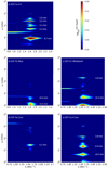 |
Fig. 6. k − ω diagrams generated from the Γ2 maps in small regions centred on the example swirls in different SOT and SST observations. Numbers denote the corresponding central periods of the patches with high FFT powers. |
The upper panel in Fig. 7 shows the variation in the average Γ2 values in the area of 18 × 18 pix2 around the centre of the SOT Ca II H example swirl (Fig. 2e), with the vertical dashed line denoting the moment of the example swirl in Fig. 2e4. Some periodicities can easily be pointed out by visual inspection. These periodicities are further confirmed by the wavelet analysis, which shows significant wavelet powers above the 95% confidence level at around 3.4, 7.0, and 14.0 min. The same approach applied to the average Γ1 values around the SOT Ca II H example swirl reveals almost identical periods at around 3.6, 7.0, and 14.0 min (first row, third column in Table 2).
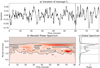 |
Fig. 7. Variation in the average Γ2 values in small regions centred on the SOT Ca II H example swirl and its wavelet spectrum. Panels a–c are similar to panels b–d in Fig. 4, except that the vertical dashed line depicts the moment of the example swirl. |
Periods in units of minutes found from the wavelet analysis in small regions centred on SOT and SST example swirls.
Table 2 lists all periods we found from the wavelet analysis of the average Γ1 and Γ2 values around the example swirls in the five passbands. Similarly as the SOT Ca II H example swirl, the periods found from the Γ1 values are almost identical to those from the Γ2 values, and most of these periods fall within the range of 3 to 14 min. When both Γ1 and Γ2 indicate the appearance of swirls, the above results suggest that in addition to the collective behaviour of swirls, the occurrence of individual swirls also exhibits periods from around 3 to 14 min.
3.3. Distribution of the periods
Figure 8 shows the distribution of periods we found in the overall parameters of photospheric swirls (panel a) and chromospheric swirls (panel b). Black dots denote the periods, and circles denote their extensions. Swirls detected from the SOT Ca II H observations were omitted from these two panels (but are included in panel c), as they might consist of photospheric and chromospheric swirls due to the complicated formation heights of the SOT Ca II H broadband filter. Except for two periods longer than 15 min among the phototopheric periods in the Hinode/SOT observations, there is no obvious difference between photospheric and chromospheric periods. Their corresponding average values are 7.1 ± 4.4 min and 6.7 ± 4.1 min. Figure 8c shows the distribution of all photospheric and chromospheric periods. It is shown again that most periods fall within the range of 3 min to 8 min. Another range of 10 min to 14 min, which is consistent with the second harmonics of the 3 min to 8 min periods, covers the second most periods. To further examine these findings, we employed a machine-learning method: the k-means clustering (MacQueen 1967), which is one of the simplest but most effective algorithms for clustering purposes. It is worth noting that k-means clustering is an unsupervised machine-learning algorithm that does not need labels. It takes a set of data as the input and automatically groups them into different clusters, among which data points in each cluster have similar properties (i.e. periods in this case).
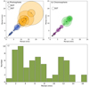 |
Fig. 8. Distributions of significant periods. Panels a and b show the distributions of periods determined from all photospheric and chromospheric swirls. The solid (dashed) black circles depict SOT (SST) swirls. Different colours denote different clusters identified by the k-means clustering algorithm (see Sect. 3). Panel c shows the histogram of all periods in all five data sets. |
The method relies on a given set of data containing n points (x1, x2, …, xn) to be divided into k clusters (S1, S2, …, Sk). The target of the k-means clustering is to separate all data into k clusters of equal variance while minimising the inertia defined as
 (1)
(1)
where μj are the centroids (average values) of each cluster. The k-clustering method was applied to photospheric periods with a k value of 2. The number 2 was chosen because we expect two main period clusters as found above. Two distinct clusters (blue and orange circles in Fig. 8a) are indeed found, with average periods of 4.6 ± 2.3 min and 12.8 ± 2.3 min, respectively. Application of the k-clustering method to the chromospheric periods reveals a very similar result. The two clusters (green and pink circles in Fig. 8b have average periods of 4.1 ± 2.1 min and 11.9 ± 1.3 min, respectively.
4. Conclusions and discussions
We conducted a statistical study of oscillations related to photospheric and chromospheric swirls detected from five SST and SOT data sets using ASDA. Periods with significant wavelet powers above their corresponding 95% confidence levels were found in the time series of the correlation coefficient (CC), the number of swirls per frame (N), the average intensity ( ), the average radius (
 ), the average rotating speed (
 ), and the average expanding/shrinking speed (
 ) of swirls detected in all five data sets. These periods range from 1 min to 17 min, with an average value of 6.9 ± 4.4 min. Two period clusters were found using the k-means clustering algorithm, one period from 3 min to 8 min, and the other from 10 min to 14 min, with the latter being approximately twice the former. More than half (∼54%) of these periods lie in or very close to the 3 min to 8 min range. Similar periods were further discovered in the Γ1 and Γ2 maps in the areas centred on five example swirls in the five different SST and SOT passbands using the FFT and wavelet analysis.
The exact relation between the 3 − 8 min and 10 − 14 min periods we found is unknown. Realistic numerical simulations might be needed to establish their physical relations. We also note that two periods shorter than 1 min are detected in the number of swirls (N), but not in other parameters (Table 1). Moreover, the longest periods found in SOT observations are overall longer than those in SST observations for the same parameters. It is unclear whether these differences are physical or artificial. Further studies are needed to investigate whether they arise because the SOT observations we used cover a longer time span.
Nevertheless, these periods in swirls recall the well-known 3 − 8 min p-mode oscillations of the Sun (e.g. Bahng & Schwarzschild 1962; Ulrich 1976; Zirker 1980), which are the result of globally coherent acoustic waves with pressure as the restoring force. Table 3 lists all significant periods from the wavelet analysis of the average intensity across the whole FOV of the SST and SOT observations. Most of the periods lie within the 5 − 8 min range (and 11 − 12 min, which are twice that of the five-minute oscillations), providing evidence that global p-mode oscillations spanning the photosphere to the chromosphere exist. These periodicities also agree well with those found in the parameters of swirls detailed in this paper. Previously, oscillations with periods of the p-mode were also observed in a large variety of structures in the solar atmosphere from the photosphere to the corona, including but not limited to sunspots (e.g. Cally et al. 2016), coronal loops (e.g. De Moortel 2006), plumes (e.g. Liu et al. 2015), and spicules (e.g. De Pontieu et al. 2004).
Periods in units of minutes found from the wavelet analysis of the average intensity throughout the entire FOV of different SOT and SST observations.
Our results suggest that the global p-mode oscillations modulate not only the occurrence manifested by periods in CC and N (and periods in the investigated example swirls), but also the properties of photospheric swirls. Chromospheric swirls have also been found to possess almost identical periods. We note that employing simultaneous photospheric and chromospheric observations and 3D numerical simulations, Liu et al. (2019b) found that photospheric swirls could trigger Alfvén pulses that propagate upward into the chromosphere and lead to the observed chromospheric swirls. This suggests that the global p-modes could play a very important role in generating photospheric swirls and thus Alfvén pulses, chromospheric swirls, and spicules, recalling that many studies have found that spicules could be driven by rotational motions at their footpoints (Oxley et al. 2020; Scalisi et al. 2021a,b; Battaglia et al. 2021). Because most photospheric swirls appear to be located at intergranular lanes (e.g. Wang et al. 1995; Bonet et al. 2008; Liu et al. 2019a), we suggest that they might be formed as a result of horizontal velocity flows (e.g. Murawski et al. 2018) that are modulated by the global p-modes. However, the exact physical processes of how photospheric swirls are formed due to global p-modes and how the vertical oscillations in the p-modes are converted into the horizontal rotations in swirls are still unclear. This may be answered by investigating realistic 3D numerical simulations similar to those in Liu et al. (2019c), where photospheric swirls were detected in the simulated photosphere undergoing p-mode oscillations.
If this scenario were proven, a new way for the global p-mode oscillation to channel both energy (via triggering Alfvén pulses) and material (via triggering spicules) into the upper solar atmosphere would be established. Here, the p-mode oscillations themselves do not need to leak into the upper solar atmosphere in inclined magnetic field lines to trigger spicules, as suggested by De Pontieu et al. (2004). Instead, they can also transport energy and mass into the upper atmosphere in less inclined magnetic lines via photospheric swirls.
Acknowledgments
Hinode is a Japanese mission developed and launched by ISAS/JAXA, with NAOJ as domestic partner and NASA and STFC (UK) as international partners. Hinode is operated by these agencies in co-operation with ESA and NSC (Norway). The Swedish s-m Solar Telescope is operated on the island of La Palma by the Institute for Solar Physics of Stockholm University in the Spanish Observatorio del Roque de los Muchachos of the Instituto de Astrofísica de Canarias. J.L. acknowledges the support from the National Key Technologies Research, Development Program of the Ministry of Science and Technology of China (2022YFF0711402) and the NSFC Distinguished Overseas Young Talents Program. D.B.J. and J.L. acknowledge support from the Leverhulme Trust via grant RPG-2019-371 and wish to thank the UK Space Agency for a National Space Technology Programme (NSTP) Technology for Space Science award (SSc 009). D.B.J. is also thankful to the UK Science and Technology Facilities Council (STFC) for grant Nos. ST/T00021X/1 and ST/X000923/1. R.E. is grateful to STFC for grant No. ST/M000826/1 and the Hungarian Scientific Research Fund (OTKA, grant No. K142987) of the National Research and Innovation Office (NKFIH), Hungary for the support received. R.E. also acknowledges the support received by the CAS Presidents International Fellowship Initiative grant No. 2019VMA052 and the Royal Society (IE161153).
References
- Attie, R., Innes, D. E., & Potts, H. E. 2009, A&A, 493, L13 [NASA ADS] [CrossRef] [EDP Sciences] [Google Scholar]
- Bahng, J., & Schwarzschild, M. 1962, AJ, 67, 267 [NASA ADS] [CrossRef] [Google Scholar]
- Balmaceda, L., Vargas Domínguez, S., Palacios, J., Cabello, I., & Domingo, V. 2010, A&A, 513, L6 [NASA ADS] [CrossRef] [EDP Sciences] [Google Scholar]
- Bate, W., Jess, D. B., Nakariakov, V. M., et al. 2022, ApJ, 930, 129 [NASA ADS] [CrossRef] [Google Scholar]
- Battaglia, A. F., Canivete Cuissa, J. R., Calvo, F., Bossart, A. A., & Steiner, O. 2021, A&A, 649, A121 [NASA ADS] [CrossRef] [EDP Sciences] [Google Scholar]
- Bonet, J. A., Márquez, I., Sánchez Almeida, J., Cabello, I., & Domingo, V. 2008, ApJ, 687, L131 [Google Scholar]
- Bonet, J. A., Márquez, I., Sánchez Almeida, J., et al. 2010, ApJ, 723, 139 [Google Scholar]
- Cally, P. S., Moradi, H., & Rajaguru, S. P. 2016, Geophys. Monograph Ser., 216, 489 [NASA ADS] [CrossRef] [Google Scholar]
- Carlsson, M., Hansteen, V. H., de Pontieu, B., et al. 2007, PASJ, 59, S663 [Google Scholar]
- Carlsson, M., Hansteen, V. H., & Gudiksen, B. V. 2009, Mem. della Soc. Astron. It., 81, 582 [NASA ADS] [Google Scholar]
- Carlsson, M., Hansteen, V. H., Gudiksen, B. V., Leenaarts, J., & De Pontieu, B. 2016, A&A, 585, A4 [NASA ADS] [CrossRef] [EDP Sciences] [Google Scholar]
- Dakanalis, I., Tsiropoula, G., Tziotziou, K., & Koutroumbas, K. 2021, Sol. Phys., 296, 17 [NASA ADS] [CrossRef] [Google Scholar]
- De Moortel, I. 2006, Philos. Trans. R. Soc. London Ser. A, 364, 461 [Google Scholar]
- De Pontieu, B., Erdélyi, R., & James, S. P. 2004, Nature, 430, 536 [Google Scholar]
- DeForest, C. E. 2004, ApJ, 617, L89 [NASA ADS] [CrossRef] [Google Scholar]
- Dey, S., Chatterjee, P., OVSN, M., et al. 2022, Nat. Phys., 18, 1 [Google Scholar]
- Fedun, V., Shelyag, S., Verth, G., Mathioudakis, M., & Erdélyi, R. 2011, Ann. Geophys., 29, 1029 [Google Scholar]
- Fisher, G. H., & Welsch, B. T. 2008, ASP Conf. Ser., 383, 373 [NASA ADS] [Google Scholar]
- Freytag, B., Steffen, M., Ludwig, H.-G., et al. 2012, J. Comput. Phys., 231, 919 [Google Scholar]
- Graftieaux, L., Michard, M., & Grosjean, N. 2001, Meas. Sci. Technol., 12, 1422 [CrossRef] [Google Scholar]
- Gudiksen, B. V., Carlsson, M., Hansteen, V. H., et al. 2011, A&A, 531, A154 [NASA ADS] [CrossRef] [EDP Sciences] [Google Scholar]
- Jess, D. B., Mathioudakis, M., Christian, D. J., Crockett, P. J., & Keenan, F. P. 2010, ApJ, 719, L134 [NASA ADS] [CrossRef] [Google Scholar]
- Jess, D. B., Van Doorsselaere, T., Verth, G., et al. 2017, ApJ, 842, 59 [Google Scholar]
- Kato, Y., & Wedemeyer, S. 2017, A&A, 601, A135 [NASA ADS] [CrossRef] [EDP Sciences] [Google Scholar]
- Kitiashvili, I. N., Kosovichev, A. G., Mansour, N. N., & Wray, A. A. 2012, ApJ, 751, 1 [Google Scholar]
- Kitiashvili, I. N., Kosovichev, A. G., Lele, S. K., Mansour, N. N., & Wray, A. A. 2013, ApJ, 770, 37 [Google Scholar]
- Kohutova, P., Verwichte, E., & Froment, C. 2020, A&A, 633, L6 [NASA ADS] [CrossRef] [EDP Sciences] [Google Scholar]
- Kosugi, T., Matsuzaki, K., Sakao, T., et al. 2007, Sol. Phys., 243, 3 [Google Scholar]
- Leonard, A. J., Mumford, S. J., Fedun, V., & Erdélyi, R. 2018, MNRAS, 480, 2839 [NASA ADS] [CrossRef] [Google Scholar]
- Liu, J., Zhou, Z., Wang, Y., et al. 2012, ApJ, 758, L26 [NASA ADS] [CrossRef] [Google Scholar]
- Liu, J., McIntosh, S. W., De Moortel, I., & Wang, Y. 2015, ApJ, 806, 273 [NASA ADS] [CrossRef] [Google Scholar]
- Liu, J., Nelson, C. J., & Erdélyi, R. 2019a, ApJ, 872, 22 [Google Scholar]
- Liu, J., Nelson, C. J., Snow, B., Wang, Y., & Erdélyi, R. 2019b, Nat. Commun., 10, 3504 [Google Scholar]
- Liu, J., Carlsson, M., Nelson, C. J., & Erdélyi, R. 2019c, A&A, 632, A97 [NASA ADS] [CrossRef] [EDP Sciences] [Google Scholar]
- MacQueen, J. 1967, Proceedings of the Ffifth Berkeley Symposium on Mathematical Statistics and Probability, 1, 281 [Google Scholar]
- Mumford, S. J., & Erdélyi, R. 2015, MNRAS, 449, 1679 [NASA ADS] [CrossRef] [Google Scholar]
- Murabito, M., Shetye, J., Stangalini, M., et al. 2020, A&A, 639, A59 [EDP Sciences] [Google Scholar]
- Murawski, K., Kayshap, P., Srivastava, A. K., et al. 2018, MNRAS, 474, 77 [NASA ADS] [CrossRef] [Google Scholar]
- Oxley, W., Scalisi, J., Ruderman, M. S., & Erdélyi, R. 2020, ApJ, 905, 168 [NASA ADS] [CrossRef] [Google Scholar]
- Rutten, R. J., de Wijn, A. G., & Sütterlin, P. 2004, A&A, 416, 333 [NASA ADS] [CrossRef] [EDP Sciences] [Google Scholar]
- Scalisi, J., Ruderman, M. S., & Erdélyi, R. 2021a, ApJ, 922, 118 [NASA ADS] [CrossRef] [Google Scholar]
- Scalisi, J., Oxley, W., Ruderman, M. S., & Erdélyi, R. 2021b, ApJ, 911, 39 [NASA ADS] [CrossRef] [Google Scholar]
- Scharmer, G. B. 2006, A&A, 447, 1111 [NASA ADS] [CrossRef] [EDP Sciences] [Google Scholar]
- Scharmer, G. B., Bjelksjo, K., Korhonen, T. K., Lindberg, B., & Petterson, B. 2003, Proc. SPIE, 4853, 341 [Google Scholar]
- Scharmer, G. B., Narayan, G., Hillberg, T., et al. 2008, ApJ, 689, L69 [Google Scholar]
- Shelyag, S., Cally, P. S., Reid, A., & Mathioudakis, M. 2013, ApJ, 776, 2011 [Google Scholar]
- Shetye, J., Verwichte, E., Stangalini, M., et al. 2019, ApJ, 881, 83 [Google Scholar]
- Shukla, P. K. 2013, J. Geophys. Res., 118, 1 [Google Scholar]
- Singh, B., Srivastava, A. K., Sharma, K., Mishra, S. K., & Dwivedi, B. N. 2022, MNRAS, 511, 4134 [NASA ADS] [CrossRef] [Google Scholar]
- Su, Y., Gömöry, P., Veronig, A., et al. 2014, ApJ, 785, L2 [NASA ADS] [CrossRef] [Google Scholar]
- Torrence, C., & Compo, G. P. 1998, Bull. Am. Meteorol. Soc., 79, 61 [Google Scholar]
- Tsuneta, S., Ichimoto, K., Katsukawa, Y., et al. 2008, Solar Phys., 249, 167 [NASA ADS] [CrossRef] [Google Scholar]
- Tziotziou, K., Tsiropoula, G., Kontogiannis, I., Scullion, E., & Doyle, J. G. 2018, A&A, 618, A51 [NASA ADS] [CrossRef] [EDP Sciences] [Google Scholar]
- Tziotziou, K., Tsiropoula, G., & Kontogiannis, I. 2019, A&A, 623, A160 [NASA ADS] [CrossRef] [EDP Sciences] [Google Scholar]
- Tziotziou, K., Tsiropoula, G., & Kontogiannis, I. 2020, A&A, 643, A166 [NASA ADS] [CrossRef] [EDP Sciences] [Google Scholar]
- Ulrich, R. K. 1976, Nat. History, 85, 73 [NASA ADS] [Google Scholar]
- Wang, Y., Noyes, R. W., Tarbell, T. D., & Title, A. M. 1995, ApJ, 447, 419 [NASA ADS] [CrossRef] [Google Scholar]
- Wedemeyer-Böhm, S., & Rouppe van der Voort, L. 2009, A&A, 507, L9 [NASA ADS] [CrossRef] [EDP Sciences] [Google Scholar]
- Wedemeyer-Böhm, S., Scullion, E., Steiner, O., et al. 2012, Nature, 486, 505 [Google Scholar]
- Welsch, B. T., Fisher, G. H., Abbett, W. P., & Regnier, S. 2004, ApJ, 610, 1148 [NASA ADS] [CrossRef] [Google Scholar]
- Yadav, N., Cameron, R. H., & Solanki, S. K. 2021, A&A, 645, A3 [NASA ADS] [CrossRef] [EDP Sciences] [Google Scholar]
- Zirker, J. B. 1980, AIAA J., 18, 176 [NASA ADS] [CrossRef] [Google Scholar]
All Tables
Periods in units of minutes found from the wavelet analysis of the overall parameters of SOT and SST photospheric and chromospheric swirls.
Periods in units of minutes found from the wavelet analysis in small regions centred on SOT and SST example swirls.
Periods in units of minutes found from the wavelet analysis of the average intensity throughout the entire FOV of different SOT and SST observations.
All Figures
|
Fig. 1. Examples of swirls detected in SST and Hinode observations. the black and white backgrounds in panels a and c are the SST Hα line core chromospheric and SOT FG blue photospheric observations on 21 June 2012 and 5 March 2007, respectively. Red and blue contours are swirls detected by ASDA (Liu et al. 2019a) with clockwise and counter-clockwise rotations, respectively. Panels b and d are the Γ2 maps, corresponding to observations in panels a and c. Γ2 values are used to define edges of swirls (see e.g. Graftieaux et al. 2001; Liu et al. 2019a). Figure axes represent physical distances across the surface of the Sun (in Mm), with the origin of the chosen domain placed at the centre of the observing FOV. |
| In the text | |
|
Fig. 2. Examples of individual swirls in SST and Hinode observations. The black and white backgrounds are the corresponding intensities at each passband. Rows 2–6 are the zoom-in views of the orange boxes in the first row. Green arrows are velocity fields estimated using FLCT. The red and blue curves are the edges of the example swirls with clockwise and counter-clockwise rotations, respectively (see main text for details). |
| In the text | |
|
Fig. 3. Flowchart of how the correlation coefficient (CC) is calculated. It1, It2, and It3 are three frames of the intensity observations. Two Γ2 maps (Γt1 and Γt2) are generated from these three intensity observations employing ASDA (Liu et al. 2019a). They are further ternarised to contain only values of −1, 0, and 1. These ternarised Γ2 maps are then used to calculate CC. For more information, see the text provided in Sect. 2. |
| In the text | |
|
Fig. 4. Variation in CC and its wavelet power spectrum. Panel a is the distribution of CC vs. time for the SST Hα line core chromospheric swirls. See Sect. 2 for the definition of the CC. The inset in panel a is a zoomed-in view of the region before the dashed green line. The dashed blue line corresponds to a CC of 0.1. Panel b shows the variation in CC after applying a highpass filter and subtracting its average value. Panel c is the corresponding wavelet power spectrum with darker colours for higher powers. The solid black curves are the local 95% confidence levels. The solid black curve in panel d is the global wavelet power. Purple text indicates peaks above the 95% confidence level (dashed black line). The dotted black lines are used to determine the extension of each peak. |
| In the text | |
|
Fig. 5. Variation in the average intensity of swirls and its wavelet spectrum. Panels a–c are similar to panels b–d in Fig. 4, but for the SST Fe I 6302 wide-band photospheric swirls. |
| In the text | |
|
Fig. 6. k − ω diagrams generated from the Γ2 maps in small regions centred on the example swirls in different SOT and SST observations. Numbers denote the corresponding central periods of the patches with high FFT powers. |
| In the text | |
|
Fig. 7. Variation in the average Γ2 values in small regions centred on the SOT Ca II H example swirl and its wavelet spectrum. Panels a–c are similar to panels b–d in Fig. 4, except that the vertical dashed line depicts the moment of the example swirl. |
| In the text | |
|
Fig. 8. Distributions of significant periods. Panels a and b show the distributions of periods determined from all photospheric and chromospheric swirls. The solid (dashed) black circles depict SOT (SST) swirls. Different colours denote different clusters identified by the k-means clustering algorithm (see Sect. 3). Panel c shows the histogram of all periods in all five data sets. |
| In the text | |
Current usage metrics show cumulative count of Article Views (full-text article views including HTML views, PDF and ePub downloads, according to the available data) and Abstracts Views on Vision4Press platform.
Data correspond to usage on the plateform after 2015. The current usage metrics is available 48-96 hours after online publication and is updated daily on week days.
Initial download of the metrics may take a while.