| Issue |
A&A
Volume 672, April 2023
|
|
|---|---|---|
| Article Number | L6 | |
| Number of page(s) | 4 | |
| Section | Letters to the Editor | |
| DOI | https://doi.org/10.1051/0004-6361/202346387 | |
| Published online | 12 April 2023 | |
Letter to the Editor
Solar oxygen abundance using SST/CRISP center-to-limb observations of the O I 7772 Å line
1
Leibniz-Institut für Astrophysik Potsdam (AIP), An der Sternwarte 16, 14482 Potsdam, Germany
e-mail: This email address is being protected from spambots. You need JavaScript enabled to view it.
2
Institute for Solar Physics, Department of Astronomy, Stockholm University, Albanova University Centre, 106 91 Stockholm, Sweden
3
Max-Planck-Institut für Astronomie, Königstuhl 17, 69117 Heidelberg, Germany
4
Scientific Computing and Research Support Unit, University of Lausanne, 1015 Lausanne, Switzerland
Received:
12
March
2023
Accepted:
3
April
2023
Abstract
Solar oxygen abundance measurements based on the O I near-infrared triplet have been a much debated subject for several decades, since non-local thermodynamic equilibrium (NLTE) calculations with 3D radiation-hydrodynamics model atmospheres introduced a large change to the 1D LTE modeling. In this work, we aim to test solar line formation across the solar disk using new observations obtained with the SST/CRISP instrument. The observed data set is based on a spectroscopic mosaic that stretches from disk center to the solar limb. By comparing the state-of-the-art 3D NLTE models with the data, we find that the 3D NLTE models provide an excellent description of the line formation across the disk. We obtain an abundance value of A(O)=(8.73 ± 0.03) dex, with a very small angular dispersion across the disk. We conclude that spectroscopic mosaics are excellent probes for geometric and physical properties of hydrodynamics models and NLTE line formation.
Key words: Sun: abundances / atomic data / radiative transfer / techniques: spectroscopic / Sun: photosphere
© The Authors 2023
 Open Access article, published by EDP Sciences, under the terms of the Creative Commons Attribution License (https://creativecommons.org/licenses/by/4.0), which permits unrestricted use, distribution, and reproduction in any medium, provided the original work is properly cited.
This article is published in open access under the Subscribe to Open model. This email address is being protected from spambots. You need JavaScript enabled to view it. to support open access publication.
1. Introduction
Oxygen (O) is the most abundant metal in the universe; its abundance is an important parameter in modern astrophysics and is widely used for determining the metallicity of galaxies (e.g., Arellano-Córdova et al. 2022). Furthermore, it influences stellar evolution (e.g., VandenBerg et al. 2012), tells us about the formation properties and history of exoplanets (e.g., Line et al. 2021), and is an important factor in stellar structure and a major contributor to stellar opacity, and thus an important ingredient for stellar models (e.g., Basu & Antia 2008). Proper and accurate measurements of the O abundance are thus critical in all of these cases. Traditionally, such methods are tested on the Sun because its disk is spatially resolved and different parts of the atmosphere can be sampled by studying the center-to-limb variation (CLV) of O lines (e.g., Delone et al. 1974; Kiselman 1993; Pereira et al. 2009; Bergemann et al. 2021).
The formation of solar O lines has been a subject of interest ever since the (believed) detection of O lines in the solar spectrum (Draper 1877; Runge & Paschen 1896; Plotkin 1977). Photospheric solar abundance studies typically focus on the O I 6300 Å and the O I near-infrared triplet. The former can be modeled in thermodynamic equilibrium (LTE) but suffers from a Ni I blend that contributes about 25% of the equivalent width (EW) of the feature and is sensitive to the treatment of convection (Allende Prieto et al. 2001; Bergemann et al. 2021). The latter lines are not significantly affected by blends but must be modeled in NLTE, as was first suggested on an empirical basis by Magain et al. (1988) and Spite & Spite (1991) for metal-poor Galactic stars on the grounds of a systematic positive difference between the abundances obtained from the permitted lines and the [O I] line. Later, the NLTE sensitivity of the 777 nm triplet was confirmed through a detailed theoretical modeling by Kiselman (1991, 1993) and Kiselman & Nordlund (1995) for the Sun. In recent years, 3D NLTE modeling has become the norm for solar photospheric abundance studies. Specifically, for O, the 3D NLTE values include (8.76 ± 0.07) dex1 by Caffau et al. (2008), (8.76 ± 0.02) dex by Steffen et al. (2015), (8.73 ± 0.05) dex by Caffau et al. (2015), (8.69 ± 0.03) dex by Amarsi et al. (2018), (8.69 ± 0.04) dex by Asplund et al. (2021), and (8.74 ± 0.03) dex by Bergemann et al. (2021). Another recent study, Magg et al. (2022), employs the O and Ni NLTE model from Bergemann et al. (2021), albeit with a different spectrum synthesis code and spatially and temporarily averaged 3D models similar to Bergemann et al. (2012). Also, less model-dependent inference methods based on 3D radiation-hydrodynamics (RHD) models have been used, for example, in Centeno & Socas-Navarro (2008), Cubas Armas et al. (2017), and Cubas Armas et al. (2020) to derive the solar O abundances of A(O)=8.86 ± 0.07 dex, 8.86 ± 0.04 dex, and 8.80 ± 0.03 dex, respectively.
In Bergemann et al. (2021), the 3D NLTE oxygen abundance was based on a spectrum with the highest spectral resolution achieved so far: the solar intensity atlas (Reiners et al. 2016) with R ≈ 700 000 provided by the Institut für Astrophysik Göttingen (IAG). An updated atlas that includes CLV is currently being prepared for public release (Ellwarth et al. 2023). However, it is worth investigating the variation in the solar profile of the O I lines at a higher spatial resolution across the spectrum because of the limited angular sampling of previous spatially resolved investigations. The aim of this work is to test the consistency of spectral line diagnostics with new Swedish 1-m Solar Telescope (SST) data and available physical models, and hence help provide more robust uncertainties on the resulting analysis of photospheric oxygen lines.
We use a new data set obtained with the CRisp Imaging SpectroPolarimeter (CRISP; Scharmer et al. 2008) at the SST (Scharmer et al. 2003) as presented in Pietrow et al. (2023). We analyze the CLV of the 7772 Å line data published by Pietrow et al. (2023) using 1D LTE, 1D NLTE, and 3D NLTE models from Bergemann et al. (2021) and discuss the implications for the solar O abundance.
2. Observations and data processing
The presented data were taken as part of a multiline CLV study by Pietrow et al. (2023). We summarize the relevant information below but refer the reader to their paper for a full overview.
The data consist of a mosaic spanning one solar radius, taken between 10:41 and 11:01 UT on 19 June 2021 with SST/CRISP. The data were reduced using a modified version of the SSTRED pipeline (de la Cruz Rodríguez et al. 2015; Löfdahl et al. 2021), which has been designed to process data from the SST. It not only includes dark and flat-field correction, but typically it also performs image restoration, removing optical aberrations caused by turbulence in the atmosphere (and partially corrected for by the SST adaptive optics) using Multi-Object Multi-Frame Blind Deconvolution (MOMFBD; Löfdahl 2002; van Noort et al. 2005). We omitted this last step, as the reconstruction can fail under poor seeing conditions (Fried parameter, r0, of 5 cm or lower).
The roughly 60″ × 1000″ mosaic was taken from the solar south pole toward the center (Fig. 1), with roughly 30% overlap between each consecutive pointing (Fig. 2). The line was sampled at ±980, ±735, ±392, ±343, ±294, ±245, ±196, ±147, ±98, ±49, and 0 mÅ at R ≈ 160 000. We recalibrated the pixel scale to 0.0584″ pixel−1 by aligning both ends of the mosaic to SDO/HMI (Scherrer et al. 2012) observations, which allows us to assign a μ value at each pixel in the mosaic. The data were then binned into 50 average profiles spaced equidistantly in μ by steps of 0.02. Finally, smoothing the data removed the effects from p-modes.
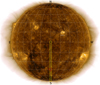 |
Fig. 1. Composite full-disk image of the Sun on 11 June 2021 in the AIA 171, 193, and 304 Å filters (Lemen et al. 2012). The yellow bar shows 25 pointings of the mosaic, which spans from the solar south pole to disk center. The red marker represents a single pointing of the telescope and has the size and orientation of SST/CRISP. |
 |
Fig. 2. Overview of the O I 7772 Å line: mosaic starting from disk center on the left and stretching to the solar limb on the right. The solid black lines show ten positions from μ = 0.1 to 1.0 (cosine of the heliocentric angle), and the dashed lines show bins of ±0.02 μ over which each μ position was averaged. The mosaic spans roughly 1000″ × 80″. |
To test the impact of limited resolving power, the data were compared to observations obtained with the Fourier Transform Spectrograph (FTS) at the IAG Vacuum Vertical Telescope (VVT), hereafter referred to as IAG FTS CLV Atlas. The resulting spectra have a resolution of 0.024 cm−1 (or R ≈ 700 000) at λ = 6000 Å (see Reiners et al. 2016; Schäfer et al. 2020; Bergemann et al. 2021). Afterward, the HITRAN (Rothman 2021) database was used to identify and mask out telluric lines from H2O and O2.
3. Methods, results, and discussion
The abundances of oxygen were calculated using the following approach. For the atmosphere, we used the 3D RHD simulations of the solar convection from the Stagger grid. We refer to Bergemann et al. (2012) and Magic et al. (2013a,b) for more details on the RHD models. The NLTE radiation transfer was carried out using the MULTI3D code (Leenaarts & Carlsson 2009), as updated in Bergemann et al. (2019) and Gallagher et al. (2020), and the new NLTE model of the oxygen atom developed in Bergemann et al. (2021). The model atom furthermore includes new oscillator strengths for the triplet lines from Bautista et al. (2022). Radiation transfer calculations were carried out using a grid of 80 × 80 × 420 points, and corrections for the finite spatial step and the lack of an overlying chromosphere were accounted for in the abundance analysis.
The line profile analysis follows Bergemann et al. (2021), where the abundance was computed via the χ2 minimization between a series of 3D NLTE line profiles calculated for the chosen μ values and the observed data. Interpolation between models computed with several values of abundance was applied. To simplify the analysis, we selected 14 μ positions with a width of ±0.02 μ from the mosaic that match the observed locations of the IAG data. We estimated the uncertainty of the abundance to be similar to the one given in Bergemann et al. (2021), although the resolution of the SST data leads to a slightly larger systematic error. Specifically, the lower sampling of the line and lower resolving power of the SST data makes it harder to correctly describe the line profile (Fig. 3), and the resulting abundance is slightly underestimated. This was tested by running the analysis on the IAG FTS CLV Atlas data degraded to the quality of SST data that can be quantified, for example, by calculating the line EW. Indeed, the EW of the SST data is somewhat lower compared to the EW of the equivalent IAG profile, yielding a ∼0.015 dex difference in the abundance. We note that the EW integration of the SST data is an unreliable procedure, especially because the sampling of the outer wings at ∼ ± 0.4 Å, where two blends are clearly visible in the original IAG data, is rather poor. A similar systematic difference is present at other angles across the disk. We accounted for the systematic bias by folding it into the absolute abundance estimate at each angle. We see a similar offset in Fig. 8 of Pietrow et al. (2023), where the trend matches data from Pereira et al. (2009) but a constant shift is found between the two sets.
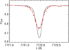 |
Fig. 3. Comparison of the observed IAG and SST line profiles for the solar disk centre. The original IAG data are shown with the solid black line. The IAG data degraded to the sampling and resolving power of the SST data are shown with filled black circles. The SST data are shown with filled red circles connected by a red line. |
The resulting oxygen abundances derived from the SST/CRISP data for 14 μ points across the solar disk are presented in Fig. 4. The average abundance obtained from the 3D NLTE modeling is very precise and independent of the viewing angle, yielding A(O)=(8.73 ± 0.031) dex. For comparison, we also show the results obtained from the 1D LTE and NLTE modeling. Clearly, these two models are unable to describe the properties of the observed solar radiation field and its CLV, overestimating the oxygen abundance by more than 0.4 dex at the limb. This supports the previous result from Bergemann et al. (2021) and reinforces the evidence that the 3D NLTE models are sufficiently complete to provide a realistic description of oxygen line formation across the disk. Hence, the abundance estimates obtained using 3D NLTE models are to be preferred for precision stellar spectroscopic diagnostics.
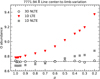 |
Fig. 4. Variation in oxygen abundance across the solar disk obtained from the SST data fitted with 3D NLTE models (open circles), a 1D LTE model (closed triangles), and a 1D NLTE model (closed squares). |
4. Conclusions
By comparing the 3D NLTE oxygen models from Bergemann et al. (2021) with our new spatially resolved SST/CRISP data, we find that the solar oxygen abundance, A(O)=(8.73 ± 0.031) dex, is fully consistent with the earlier result. Our data do not reveal any angular dependence of abundance, further demonstrating the accuracy of the 3D NLTE modeling approach as compared to 1D modeling. The abundance is consistent with the value from Amarsi et al. (2018) within the respective uncertainties of both estimates. The difference between their study and our result is indeed rather modest given the differences in the choice of observations, gf values, and correction for the chromospheric back-heating, as well the different 3D NLTE codes and the NLTE model of O. We conclude that the CLV data sets from Pietrow et al. (2023) and those of the IAG FTS CLV Atlas complement each other and synergistically probe the geometric and physical properties of RHD models of stellar convection and NLTE line formation. However, higher resolution spectral data are preferred where possible for precision solar abundance diagnostics.
We adopted the traditional astronomical logarithmic abundance scale A(ϵ)=12 + log10(nϵ/nH), which expresses the abundance of element “ϵ” on a logarithmic scale relative to nH = 1012 hydrogen atoms.
Acknowledgments
AP was supported at AIP by grants the European Commission’s Horizon 2020 Program under grant agreements 824064 (ESCAPE – European Science Cluster of Astronomy & Particle Physics ESFRI Research Infrastructures) and 824135 (SOLARNET – Integrating High Resolution Solar Physics). The CHROMATIC project (2016.0019) of the Knut and Alice Wallenberg foundation supported AP at SU. MB is supported through the Lise Meitner grant from the Max-Planck Gesellschaft. We acknowledge support by the Collaborative Research center SFB 881 at Universität Heidelberg (projects A5, A10) of the Deutsche Forschungsgemeinschaft (DFG). MB received funding from the European Research Council (ERC) as part of the European Commission’s Horizon 2020 program under grant agreement 949173. We thank Carsten Denker for his feedback on the manuscript text and the anonymous referee for their valuable suggestions during the peer-review process. The Swedish 1-m Solar Telescope is operated on the island of La Palma by the Institute for Solar Physics of Stockholm University in the Spanish Observatorio del Roque de los Muchachos of the Instituto de Astrofísica de Canarias. The Institute for Solar Physics was supported by a grant for research infrastructures of national importance from the Swedish Research Council (registration number 2017-00625). This research has made use of NASA’s Astrophysics Data System (ADS) bibliographic services. We acknowledge the community efforts devoted to the development of the following open-source packages that were used in this work: numpy (https://numpy.org/), matplotlib (https://matplotlib.org/), and astropy (https://www.astropy.org/). We extensively used the CRISPEX analysis tool (Vissers & Rouppe van der Voort 2012), the ISPy library (Díaz Baso et al. 2021), and SOAImage DS9 (Joye & Mandel 2003) for data visualization.
References
- Allende Prieto, C., Lambert, D. L., & Asplund, M. 2001, ApJ, 556, L63 [Google Scholar]
- Amarsi, A. M., Barklem, P. S., Asplund, M., Collet, R., & Zatsarinny, O. 2018, A&A, 616, A89 [NASA ADS] [CrossRef] [EDP Sciences] [Google Scholar]
- Arellano-Córdova, K. Z., Berg, D. A., Chisholm, J., et al. 2022, ApJ, 940, L23 [CrossRef] [Google Scholar]
- Asplund, M., Amarsi, A. M., & Grevesse, N. 2021, A&A, 653, A141 [NASA ADS] [CrossRef] [EDP Sciences] [Google Scholar]
- Basu, S., & Antia, H. M. 2008, Phys. Rep., 457, 217 [Google Scholar]
- Bautista, M. A., Bergemann, M., Gallego, H. C., et al. 2022, A&A, 665, A18 [NASA ADS] [CrossRef] [EDP Sciences] [Google Scholar]
- Bergemann, M., Lind, K., Collet, R., Magic, Z., & Asplund, M. 2012, MNRAS, 427, 27 [Google Scholar]
- Bergemann, M., Gallagher, A. J., Eitner, P., et al. 2019, A&A, 631, A80 [NASA ADS] [CrossRef] [EDP Sciences] [Google Scholar]
- Bergemann, M., Hoppe, R., Semenova, E., et al. 2021, MNRAS, 508, 2236 [NASA ADS] [CrossRef] [Google Scholar]
- Caffau, E., Steffen, M., & Ludwig, H. G. 2008, Eur. Sol. Phys. Meet., 12, 3.7 [NASA ADS] [Google Scholar]
- Caffau, E., Ludwig, H. G., Steffen, M., et al. 2015, A&A, 579, A88 [NASA ADS] [CrossRef] [EDP Sciences] [Google Scholar]
- Centeno, R., & Socas-Navarro, H. 2008, ApJ, 682, L61 [NASA ADS] [CrossRef] [Google Scholar]
- Cubas Armas, M., Asensio Ramos, A., & Socas-Navarro, H. 2017, A&A, 600, A45 [NASA ADS] [CrossRef] [EDP Sciences] [Google Scholar]
- Cubas Armas, M., Asensio Ramos, A., & Socas-Navarro, H. 2020, A&A, 643, A142 [NASA ADS] [CrossRef] [EDP Sciences] [Google Scholar]
- de la Cruz Rodríguez, J., Löfdahl, M. G., Sütterlin, P., Hillberg, T., & Rouppe van der Voort, L. 2015, A&A, 573, A40 [NASA ADS] [CrossRef] [EDP Sciences] [Google Scholar]
- Delone, A. B., Zakharova, A. L., & Sitnik, G. F. 1974, Sov. Astron., 17, 557 [NASA ADS] [Google Scholar]
- Díaz Baso, C. J., Vissers, G., Calvo, F., et al. 2021, https://zenodo.org/record/5608441 [Google Scholar]
- Draper, H. 1877, Am. J. Sci., 14, 89 [NASA ADS] [Google Scholar]
- Ellwarth, M., Schäfer, S., Reiners, A., & Zechmeister, M. 2023, A&A, in press https://doi.org/10.1051/0004-6361/202245612 [Google Scholar]
- Gallagher, A. J., Bergemann, M., Collet, R., et al. 2020, A&A, 634, A55 [NASA ADS] [CrossRef] [EDP Sciences] [Google Scholar]
- Joye, W. A., & Mandel, E. 2003, in Astronomical Data Analysis Software and Systems XII, eds. H. E. Payne, R. I. Jedrzejewski, & R. N. Hook, ASP Conf. Ser., 295, 489 [NASA ADS] [Google Scholar]
- Kiselman, D. 1991, A&A, 245, L9 [NASA ADS] [Google Scholar]
- Kiselman, D. 1993, A&A, 275, 269 [Google Scholar]
- Kiselman, D., & Nordlund, A. 1995, A&A, 302, 578 [Google Scholar]
- Leenaarts, J., & Carlsson, M. 2009, in The Second Hinode Science Meeting: Beyond Discovery-Toward Understanding, eds. B. Lites, M. Cheung, T. Magara, J. Mariska, & K. Reeves, ASP Conf. Ser., 415, 87 [Google Scholar]
- Lemen, J. R., Title, A. M., Akin, D. J., et al. 2012, Sol. Phys., 275, 17 [Google Scholar]
- Line, M. R., Brogi, M., Bean, J. L., et al. 2021, Nature, 598, 580 [NASA ADS] [CrossRef] [Google Scholar]
- Löfdahl, M. G. 2002, in Image Reconstruction from Incomplete Data II, eds. P. J. Bones, M. A. Fiddy, & R. P. Millane, Proc SPIE, 4792, 146 [Google Scholar]
- Löfdahl, M. G., Hillberg, T., de la Cruz Rodríguez, J., et al. 2021, A&A, 653, 653 [Google Scholar]
- Magain, P. 1988, in The Impact of Very High S/N Spectroscopy on Stellar Physics, ed. M. Spite , 132, 485 [NASA ADS] [CrossRef] [Google Scholar]
- Magg, E., Bergemann, M., Serenelli, A., et al. 2022, A&A, 661, A140 [NASA ADS] [CrossRef] [EDP Sciences] [Google Scholar]
- Magic, Z., Collet, R., Asplund, M., et al. 2013a, A&A, 557, A26 [NASA ADS] [CrossRef] [EDP Sciences] [Google Scholar]
- Magic, Z., Collet, R., Hayek, W., & Asplund, M. 2013b, A&A, 560, A8 [NASA ADS] [CrossRef] [EDP Sciences] [Google Scholar]
- Pereira, T. M. D., Asplund, M., & Kiselman, D. 2009, A&A, 508, 1403 [NASA ADS] [CrossRef] [EDP Sciences] [Google Scholar]
- Pietrow, A. G. M., Kiselman, D., Andriienko, O., et al. 2023, A&A, 671, 671 [Google Scholar]
- Plotkin, H. 1977, J. Hist. Astron., 8, 44 [NASA ADS] [CrossRef] [Google Scholar]
- Reiners, A., Mrotzek, N., Lemke, U., Hinrichs, J., & Reinsch, K. 2016, A&A, 587, A65 [NASA ADS] [CrossRef] [EDP Sciences] [Google Scholar]
- Rothman, L. S. 2021, Nat. Rev. Phys., 3, 302 [CrossRef] [Google Scholar]
- Runge, C., & Paschen, F. 1896, ApJ, 4, 317 [NASA ADS] [CrossRef] [Google Scholar]
- Schäfer, S., Royen, K., Huster Zapke, A., Ellwarth, M., & Reiners, A. 2020, in Ground-based and Airborne Instrumentation for Astronomy VIII, eds. C. J. Evans, J. J. Bryant, & K. Motohara, Proc. SPIE, 11447, 11447A9 [Google Scholar]
- Scharmer, G. B., Bjelksjo, K., Korhonen, T. K., Lindberg, B., & Petterson, B. 2003, in Innovative Telescopes and Instrumentation for Solar Astrophysics, eds. S. L. Keil, & S. V. Avakyan , Proc. SPIE, 4853, 341 [NASA ADS] [CrossRef] [Google Scholar]
- Scharmer, G. B., Narayan, G., Hillberg, T., et al. 2008, ApJ, 689, L69 [Google Scholar]
- Scherrer, P. H., Schou, J., Bush, R. I., et al. 2012, Sol. Phys., 275, 207 [Google Scholar]
- Spite, M., & Spite, F. 1991, A&A, 252, 689 [NASA ADS] [Google Scholar]
- Steffen, M., Prakapavičius, D., Caffau, E., et al. 2015, A&A, 583, A57 [NASA ADS] [CrossRef] [EDP Sciences] [Google Scholar]
- VandenBerg, D. A., Bergbusch, P. A., Dotter, A., et al. 2012, ApJ, 755, 15 [Google Scholar]
- van Noort, M., Rouppe van der Voort, L., & Löfdahl, M. G. 2005, Sol. Phys., 228, 191 [Google Scholar]
- Vissers, G., & Rouppe van der Voort, L. 2012, ApJ, 750, 22 [Google Scholar]
All Figures
|
Fig. 1. Composite full-disk image of the Sun on 11 June 2021 in the AIA 171, 193, and 304 Å filters (Lemen et al. 2012). The yellow bar shows 25 pointings of the mosaic, which spans from the solar south pole to disk center. The red marker represents a single pointing of the telescope and has the size and orientation of SST/CRISP. |
| In the text | |
|
Fig. 2. Overview of the O I 7772 Å line: mosaic starting from disk center on the left and stretching to the solar limb on the right. The solid black lines show ten positions from μ = 0.1 to 1.0 (cosine of the heliocentric angle), and the dashed lines show bins of ±0.02 μ over which each μ position was averaged. The mosaic spans roughly 1000″ × 80″. |
| In the text | |
|
Fig. 3. Comparison of the observed IAG and SST line profiles for the solar disk centre. The original IAG data are shown with the solid black line. The IAG data degraded to the sampling and resolving power of the SST data are shown with filled black circles. The SST data are shown with filled red circles connected by a red line. |
| In the text | |
|
Fig. 4. Variation in oxygen abundance across the solar disk obtained from the SST data fitted with 3D NLTE models (open circles), a 1D LTE model (closed triangles), and a 1D NLTE model (closed squares). |
| In the text | |
Current usage metrics show cumulative count of Article Views (full-text article views including HTML views, PDF and ePub downloads, according to the available data) and Abstracts Views on Vision4Press platform.
Data correspond to usage on the plateform after 2015. The current usage metrics is available 48-96 hours after online publication and is updated daily on week days.
Initial download of the metrics may take a while.