| Issue |
A&A
Volume 672, April 2023
|
|
|---|---|---|
| Article Number | A98 | |
| Number of page(s) | 8 | |
| Section | Extragalactic astronomy | |
| DOI | https://doi.org/10.1051/0004-6361/202345924 | |
| Published online | 06 April 2023 | |
The co-evolution of supermassive black holes and galaxies in luminous AGN over a wide range of redshift
Instituto de Fisica de Cantabria (CSIC-Universidad de Cantabria), Avenida de los Castros, 39005 Santander, Spain
e-mail: This email address is being protected from spambots. You need JavaScript enabled to view it.
Received:
17
January
2023
Accepted:
20
February
2023
Abstract
It is well known that supermassive black holes (SMBHs) and their host galaxies co-evolve. A manifestation of this co-evolution is the correlation that has been found between the SMBH mass, MBH, and the galaxy bulge or stellar mass, M*. The cosmic evolution of this relation, though, is still a matter of debate. In this work, we examine the MBH − M* relation, using 687 X-ray luminous (median log [LX,2−10 keV(erg s−1)] = 44.3), broad-line active galactic nuclei (AGN), at 0.2 < z < 4.0 (median z ≈ 1.4) that lie in the XMM-XXL field. Their MBH and M* range from 7.5 < log [MBH (M⊙)] < 9.5 and 10 < log [M*(M⊙)] < 12, respectively. Most of the AGN live in star-forming galaxies and their Eddington ratios range from 0.01 to 1, with a median value of 0.06. Our results show that MBH and M* are correlated (r = 0.47 ± 0.21, averaged over different redshift intervals). Our analysis also shows that the mean ratio of the MBH and M* does not evolve with redshift, at least up to z = 2 and has a value of log(MBH/M*)= − 2.44. The majority of the AGN (75%) are in a SMBH mass growth-dominant phase. In these systems, the MBH − M* correlation is weaker and their M* tends to be lower (for the same MBH) compared to systems that are in a galaxy mass growth phase. Our findings suggest that the growth of black hole mass occurs first, while the early stellar mass assembly may not be so efficient.
Key words: galaxies: active / galaxies: evolution / quasars: supermassive black holes / galaxies: star formation / X-rays: galaxies
© The Authors 2023
 Open Access article, published by EDP Sciences, under the terms of the Creative Commons Attribution License (https://creativecommons.org/licenses/by/4.0), which permits unrestricted use, distribution, and reproduction in any medium, provided the original work is properly cited.
This article is published in open access under the Subscribe to Open model. This email address is being protected from spambots. You need JavaScript enabled to view it. to support open access publication.
1. Introduction
In the last two decades, several studies have shown that there is a co-evolution between the supermassive black holes (SMBHs) and their host galaxies (e.g., Kormendy & Ho 2013). In the local Universe, this co-evolution has been demonstrated by tight correlations that have been found between the SMBH mass, MBH, and various properties of the host galaxy. For instance, there is a correlation between the MBH and the stellar velocity dispersion, the bulge luminosity, and the bulge mass, Mbulge (e.g., Magorrian et al. 1998; Ferrarese & Merritt 2000; Gebhardt et al. 2000; Tremaine et al. 2002; Häring & Rix 2004). Among them, the correlation between the MBH and the velocity dispersion of the galaxy bulge (σ) appears to be the tightest. A possible explanation could be that σ is a good predictor of Mbulge. Another, perhaps more plausible, scenario is that σ measures the depth of the potential well in which the SMBH is formed (Ferrarese & Merritt 2000).
Although these correlations are well established at low redshift (z < 1), it is still unclear if and how they evolve at high redshifts. A comparison of the local scaling relations with those at higher redshifts is not straightforward. Shankar et al. (2016) used Monte Carlo simulations and found evidence that local galaxy samples with dynamically measured MBH may suffer from an angular resolution related selection effect that could bias the observed scaling relations between the MBH and galaxy properties. However, this selection effect does not affect local samples of active galactic nuclei (AGN; Shankar et al. 2019).
The MBH and Mbulge or stellar mass, M*, is one of the most extensively studied relations, both from a theoretical as well as from an observational point of view (e.g., Marconi & Hunt 2003; Gültekin et al. 2009; Sani et al. 2011; Reines & Volonteri 2015). Since, at high redshift, it is difficult to separate the bulge from the total stellar mass, many observational works at z ≥ 1 have studied the MBH − M* relation (e.g., Jahnke et al. 2009; Merloni et al. 2010; Schramm & Silverman 2013; Sun et al. 2015; Suh et al. 2020; Setoguchi et al. 2021; Poitevineau et al. 2023) as opposed to the MBH − Mbulge that is often studied at z < 1 (e.g., Park et al. 2015).
For the majority of the aforementioned observational studies, the MBH − M* relation has been examined for broad-line AGN (BLAGN1) whose MBH were measured using continuum luminosities and broad-line widths. Jahnke et al. (2009) used ten AGN in the COSMOS field at 1 < z < 2 and found no difference between their MBH − M* relation and that in the local Universe. Merloni et al. (2010) used 89 broad-line AGN in the zCOSMOS survey at 1 < 1 < 2.2 and found that the MBH/M* ratio evolves with redshift. Schramm & Silverman (2013) used 18 X-ray selected, broad-line AGN at 0.5 < z < 1.2 and found that bulge-dominated host galaxies are more aligned with the local relation than those with prominent discs. Sun et al. (2015) used 69 Herschel detected, broad-line AGN at 0.2 ≤ z < 2.1 and found that galaxies with overmassive (undermassive) black holes (BHs) tend to have a low (high) ratio of the specific accretion rate to the specific star formation rate. Suh et al. (2020) used a sample of 100 X-ray selected, broad-line and moderate luminosity AGN in the Chandra-COSMOS Legacy survey up to z ∼ 2.5 and found no significant evolution of the MBH/M* ratio. Setoguchi et al. (2021) used 117, moderate luminosity, broad-line AGN in the Subaru/XMM-Newton Deep Field (SXDF) and found that the MBH/M* ratio is similar to that in the local Universe. According to the authors, if their galaxies are bulge dominant, then they have already established the local MBH − M* relation. If they are disc dominant, then their SMBHs are overmassive relative to their M*.
In most of the above works, a limiting factor is the relatively small number of AGN (⪅100) used in the analysis. Furthermore, the examination of the evolution of the MBH − M* relation with redshift is done my comparing and combining results from different studies. This approach, though, may hint at systematic effects. Although, the calculation of MBH at different redshifts and therefore using widths of different broad lines (Hβ, Mg II, and C IV) gives consistent results (e.g., Shen et al. 2013; Liu et al. 2016), this is not true for the measurement of the galaxy properties, such as the M* and the star formation rate (SFR). In this case, utilising different methods and/or different templates and parameter space – for example when fitting their spectral energy distribution (SED) – may introduce a number of systematics that could affect the comparison and thus the overall conclusions (Mountrichas et al. 2021b).
In this work, we use 687 X-ray selected, broad-line and luminous (median log [LX,2−10 keV(erg s−1)] = 44.3) AGN that span a redshift range of 0.2 < z < 4.0 to study the correlation between the AGN and their host galaxy properties at different redshift intervals. In Sect. 2 we describe the parent sample and the strict criteria we applied to compile a final dataset with accurate and consistent AGN and galaxy measurements. The results are presented in Sect. 3 and we summarise our main conclusions in Sect. 4. Throughout this work, we assume a flat ΛCDM cosmology with H0 = 70.4 km s−1 Mpc−1 and ΩM = 0.272 (Komatsu et al. 2011).
2. Data
In this section, we describe the XMM-XXL survey and how we obtained measurements for important AGN and host galaxy properties that are used throughout this work.
2.1. The sample
The X-ray AGN used in this study were observed in the northern field of the XMM-Newton-XXL survey (XMM-XXL; Pierre et al. 2016). XMM-XXL is a medium-depth X-ray survey that covers a total area of 50 deg2 split into two fields equal in size, the XMM-XXL North (XXL-N) and the XMM-XXL South (XXL-S). The XXL-N sample consists of 8445 X-ray sources. Of these X-ray sources, 5294 have SDSS counterparts and 2512 have reliable spectroscopy (Menzel et al. 2016; Liu et al. 2016). Mid-IR and near-IR was obtained following the likelihood ratio method (Sutherland & Saunders 1992) as implemented in Georgakakis & Nandra (2011). For more details on the reduction of the XMM observations and the IR identifications of the X-ray sources, readers can refer to Georgakakis et al. (2017).
2.2. Black hole mass measurements
As mentioned above, there are 2512 AGN in the XXL-N catalogue that have reliable spectroscopy from SDSS-III/BOSS. In particular, 1786 out of these 2512 sources have been classified as BLAGN1, by Menzel et al. (2016). A source was classified as BLAGN1 using the full width at half-maximum (FWHM) threshold of 1000 Km s−1. Liu et al. (2016) performed spectral fits to the BOSS spectroscopy of these 1786 BLAGN1 to estimate single-epoch virial MBH from continuum luminosities and broad line widths (e.g., Shen et al. 2013). The details of the spectral fitting procedure are given in Sect. 3.3 of Liu et al. (2016) and in Shen et al. (2013). In brief, they first measured the continuum luminosities and broad-line FWHMs. Then, they used several single-epoch virial mass estimators to calculate MBH. Specifically, they applied the following fiducial mass recipes, depending on the redshift of the source: H β at z < 0.9, Mg II at 0.9 < z < 2.2, and C IV at z > 2.2.
Previous studies have shown that single-epoch MBH estimates that use different emission lines, when adopting the fiducial single-epoch mass formula, are generally consistent with each other with negligible systematic offsets and scatter (e.g., Shen et al. 2008, 2011, 2013; Shen & Liu 2012). Liu et al. (2016) confirmed these previous findings. Finally, their MBH measurements have, on average, errors of ∼0.5 dex, whereas sources with higher signal-to-noise ratio (S/N) have uncertainties of the measured MBH that are less than 0.15 dex.
2.3. Host galaxy measurements
In our analysis, we use the host galaxy measurements presented in Mountrichas & Shankar (2023). These have been derived by applying spectral energy distribution (SED) fitting, using the CIGALE code (Boquien et al. 2019; Yang et al. 2020, 2022). The available photometry has been compiled and presented in Masoura et al. (2018, 2021). The templates and parameter space used is the same as that presented in Mountrichas et al. (2021b), Mountrichas et al. (2022a,c). In brief, a delayed star formation history (SFH) model with a function form SFR ∝ t × exp(−t/τ) was used to fit the galaxy component. A star formation burst was included (Ciesla et al. 2017; Małek et al. 2018; Buat et al. 2019) as a constant ongoing period of star formation of 50 Myr. The Bruzual & Charlot (2003) single stellar population template was used to model the stellar emission. Stellar emission was attenuated following Charlot & Fall (2000). The dust heated by stars was modelled following Dale et al. (2014). The SKIRTOR template (Stalevski et al. 2012, 2016) was used for the AGN emission. Accounting for the AGN emission significantly reduced the biases on the estimate of the M* and SFR of their host galaxy (Ciesla et al. 2015). The values for the various parameters are similar to those presented in Tables 1 in Mountrichas et al. (2021b), Mountrichas et al. (2022a,c).
To examine if our SFR and M* measurements are sensitive to the adopted SFH model, we repeated the SED fitting process using a different SFH module. Specifically, we adopted an expansion of the delayed SFH model mentioned above, which allows for a recent quenching of the SFR (Ciesla et al. 2017). This module is provided as sfhdelayedbq in CIGALE. We confirm that CIGALE measurements for the host galaxy properties of interest are robust and do not depend on the selection of the SFH model (see also Appendix B in Mountrichas et al. 2022a).
2.4. Final sample
To ensure that only sources with reliable galaxy measurements are included in our analysis, we followed the criteria used in our previous studies (Mountrichas et al. 2021b, 2022a, 2022c; Mountrichas & Shankar 2023). Specifically, we have included only sources that have measurements in the following photometric bands: u, g, r, i, z, J, H, K, W1, W2, and W4, where W1, W2, and W4 are the WISE photometric bands at 3.4, 4.6, and 22 μm, respectively. Approximately, 50% of our sources have far-IR measurements by Herschel (HELP collaboration; Shirley et al. 2019, 2021). However, previous studies have shown that a lack of far-IR photometry does not affect the SFR calculations of CIGALE (Mountrichas et al. 2021a, 2021b, 2022a; Mountrichas et al. 2022c). Therefore, we did not require our sources to have available far-IR photometry.
Furthermore, we excluded sources with bad SED fits and unreliable host galaxy measurements. To this end, we imposed a reduced χ2 threshold of χr2 < 5 (e.g., Masoura et al. 2018; Buat et al. 2021). We also excluded systems for which CIGALE could not constrain the parameters of interest (SFR and M*). For that, we applied the same criteria used in previous recent studies (e.g., Mountrichas et al. 2021b, 2022b, 2022c; Buat et al. 2021; Koutoulidis et al. 2022). The method uses the two values that CIGALE provides for each estimated galaxy property. One value corresponds to the best model and the other value (bayes) is the likelihood-weighted mean value. A large difference between the two calculations suggests a complex likelihood distribution and important uncertainties. Therefore, in our analysis, we have only included sources with  and
and  , where SFRbest and M*, best are the best-fit values of SFR and M*, respectively, and SFRbayes and M*, bayes are the Bayesian values estimated by CIGALE. These criteria reduce the number of X-ray AGN to 1592. We note that this number includes sources with either spectroscopic or photometric redshifts (photoz). The photoz calculations have been presented in Masoura et al. (2018).
We then cross matched these 1592 AGN with the spectroscopic sample of Liu et al. (2016). This results in 687 broad-line, X-ray AGN with spectroscopic redshifts that have reliable measurements for MBH and galaxy properties. The distribution of MBH and M* vs. redshift for our final AGN sample is presented in the top and bottom panels of Fig. 1, respectively. The X-ray luminosity of the sources spans a range of 42.5 < log [LX,2−10 keV(erg s−1)] < 45.5 with a median value of log [LX,2−10 keV(erg s−1)] = 44.3. The median redshift is z = 1.4 (0.2 < z < 4.0). To minimise selection effects in our analysis (see next sections), we split the dataset into four redshift intervals. There are 181 AGN at z < 0.9, 215 at 0.9 < z < 1.5, 188 at 1.5 < z < 2.2, and 103 AGN at z > 2.2.
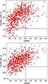 |
Fig. 1. SMBH and galaxy properties as a function of redshift. Top panel: MBH vs. redshift. Bottom panel: M* vs. redshift. The dashed horizontal lines show the MBH (top panel) and M* (bottom panel) limits to which our sample is complete up to redshift 2 (vertical lines). For more details, readers can refer to Sect. 3.3. |
There are two available measurements for the bolometric luminosities, Lbol, of our sources. The catalogue of Liu et al. (2016) includes Lbol calculations. For their estimation, they have integrated the radiation directly produced by the accretion process, that is the thermal emission from the accretion disc and the hard X-ray radiation produced by inverse-Compton scattering of the soft disc photons by a hot corona (for more details see their Sect. 4.2). We also combined CIGALE’s measurements for the absorption-corrected X-ray luminosity and the AGN disc luminosity. Comparison of the two Lbol estimates shows that the distribution of their (log) difference has a mean value of 0.08 dex and a standard deviation of 0.42 dex. In our analysis, we have chosen to use the Lbol calculations of CIGALE. However, we confirm that this choice does not affect our overall results and conclusions.
3. Results and discussion
3.1. SFR versus M*
The SFR–M* relation of our sources is presented in Fig. 2. Different symbols correspond to different redshift intervals, as indicated in the legend. The results are colour-coded based on the MBH. Sources located in the upper right corner of the SFR–M* space, with log [SFR(M⊙ yr−1)] > 3 and log [M*(M⊙)] > 12, are high-redshift sources (z > 2) with massive SMBHs (log [MBH (M⊙)] > 9). Based on the specific SFR, sSFR (sSFR = SFR/M*), measurements of CIGALE, there is only a small number of AGN in our dataset that are in quiescent systems (log sSFR(Gyr−1)> 11). The vast majority of our AGN are either in star-forming or in starburst galaxies. We note that we chose to identify quiescent systems based on their sSFR values as opposed to overploting a main sequence, MS, from the literature (e.g., Whitaker et al. 2014; Schreiber et al. 2015) due to the systematics that this approach may introduce (for more details see e.g., Mountrichas et al. 2021b).
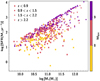 |
Fig. 2. SFR vs. M* of the X-ray AGN in our dataset. Different symbols indicate different redshift intervals, as shown in the legend. The results are colour-coded based on the MBH value. |
Most previous studies have found a strong, positive correlation between the SFR and the X-ray luminosity of AGN (e.g., Lanzuisi et al. 2017; Masoura et al. 2018, 2021), although more recent works have shown that this correlation is weaker when systematic effects are minimised and when the M* is taken into account (e.g., Mountrichas et al. 2021b, 2022c, 2022a). Recently, Bluck et al. (2023) analysed three cosmological hydrodynamical simulations (Eagle, Illustris, and IllustrisTNG) and they conclude that the MBH is the predictive parameter of galaxy quenching and not the AGN luminosity. We applied Pearson correlation analysis, splitting our data into the four redshift intervals shown in the legend of Fig. 2. The results show that the sSFR and X-ray luminosity (or Lbol) have an (average over the four redshift bins) correlation coefficient of r = 0.45 ± 0.15 (or r = 0.37 ± 0.22). The correlation coefficient of the sSFR and MBH is r = 0.31 ± 0.12. The errors are the standard deviations. These results, although indicative, corroborate that observational works should examine the role of MBH when studying the impact of AGN feedback on the host galaxy properties, as suggested by Bluck et al. (2023).
3.2. Lbol versus MBH
In Fig. 3, we plot the Lbol calculations of CIGALE as a function of MBH for the different redshift intervals used in our study. The lines correspond to Lbol = LEdd (green long-dashed line), Lbol = 0.1 LEdd (solid black line), and Lbol = 0.01 LEdd (grey dashed line), where LEdd = 1.26 × 1038MBH/M⊙ erg s−1. The vast majority of our AGN lie between Eddington ratios of 0.01–1, with a median value of 0.06, which is in agreement with previous studies (e.g., Trump et al. 2009; Lusso et al. 2012; Sun et al. 2015; Suh et al. 2020). The fact that the SMBHs of the X-ray luminous AGN in our dataset accrete at sub-Eddington rates at all redshifts spanned by our sample could indicate that most of their mass has been built up at earlier epochs.
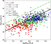 |
Fig. 3. Lbol as a function of MBH. Different symbols and colours correspond to different redshift intervals, as indicated in the legend. The lines correspond to Lbol = LEdd (green long-dashed line), Lbol = 0.1 LEdd (solid black line), and Lbol = 0.01 LEdd (grey short-dashed line). |
3.3. The MBH − M* relation
In this section, we examine the MBH − M* relation and the evolution of the MBH/M* ratio with redshift. The top panel of Fig. 4 presents the MBH measurements of the AGN as a function of their host galaxy M*. Symbols are colour coded based on the redshift interval to which the source belongs. The solid black line presents the best fit of our measurements (MBH = 1.054 M* − 3.010). In the same panel, we also present the best fits from previous studies. The orange dashed line shows the best fit from Häring & Rix (2004). In that study, the authors examined the BH−bulge mass relation, using a sample of 30 nearby galaxies. The purple long-dashed line presents the best fit from Kormendy & Ho (2013) for local, bulge galaxies. The grey dashed line is the best fit found by Suh et al. (2020), which combined their sample of 100 X-ray selected AGN in the Chandra-COSMOS Legacy Survey which spanned a redshift range up to 2.5, with the sample presented in Reines & Volonteri (2015) which consists of nearby, inactive early-type galaxies as well as local AGN.
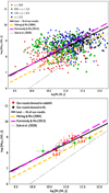 |
Fig. 4. MBH as a function of M*. The top panel shows the distribution of our AGN in the MBH − M* space. Different colours correspond to different redshift bins. The bottom panel shows our results grouped in bins of redshift (red symbols) and M* (green symbols). Median values are presented as well as the 1σ uncertainties (calculated via bootstrap resampling). The labels next to the red points show the median redshift that corresponds to each bin. The solid black line shows the best fit on our measurements. The dashed lines, in both panels, present the best fits from previous studies (see text for more details). |
We applied a correlation analysis and we found a correlation coefficient of r = 0.47 ± 0.21 between the two properties for the sources in our sample. This value was averaged over the four redshift intervals. The error presents the standard deviation of the four measurements. This result is consistent with the value we calculated using the M* and MBH measurements presented in Table 2 in Sun et al. (2015) that have a median redshift of ≈1.2 (r = 0.43). It is also consistent with MBH − M* correlations reported in the local Universe (e.g., 0.54; Reines & Volonteri 2015). The correlation coefficients of our MBH and M* for each of the redshift bins are: 0.31, 0.35, 0.38, and 0.36 at z < 0.9, 0.9 < z < 1.5, 1.5 < z < 2.2, and z > 2.2, respectively. Although, the coefficient values are consistent across all redshifts spanned by our dataset, they appear a bit lower compared to the correlation coefficient of the full sample. This is, probably, mostly due to the smaller MBH ranges spanned by the individual redshift bins compared to the full catalogue. The bottom panel of Fig. 4 presents the results when we binned the MBH and M* into the four redshift bins we used in our analysis (red circles). The median MBH and M* values and their 1σ uncertainties (calculated via bootstrap resampling) are shown. We also binned our M* and MBH calculations in four M* bins within 10 < log [M*(M⊙)] < 12 (green circles). Each bin has a 0.5 dex width.
Next, we examine the MBH/M* ratio as a function of redshift. Based on the results presented in the top panel of Fig. 5, the MBH/M* ratio does not evolve with redshift. The mean log(MBH/M*) value is found at −2.44 (with a 1σ scatter of 0.61), shown by the dashed line. The scatter of the log(MBH/M*) ratio is similar at all redshifts spanned by the dataset. Specifically, σ ∼ 0.6 up to redshift 2.2 and σ ∼ 0.45 at z > 2.2. The value of the log(MBH/M*) ratio is in agreement with that found by Setoguchi et al. (2021; −2.2), but somewhat higher compared to that found by Suh et al. (2020; ≈ − 2.7) and that found in the local Universe (−2.85; Häring & Rix 2004).
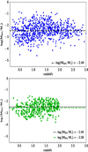 |
Fig. 5. MBH − M* ratio as a function of redshift. The top panel shows the values for the total AGN sample. The bottom panel shows the results when we accounted for selection biases (see text for more details). The horizontal dashed black line in both panels indicates the mean MBH − M* ratio value of our dataset. The horizontal long-dashed green line presents the mean MBH − M* ratio value, when selection biases are taken into consideration. |
We note that our dataset is a high-redshift, flux-limited sample and this makes it susceptible to suffer from Eddington bias. However, as has been pointed out, for instance in Poitevineau et al. (2023), both MBH and M* scale with with BLR line and the IR-to-optical luminosities, respectively, and thus have a similar dependence on redshift. Furthermore, the MBH/M* ratio spans a wide range, at least up to redshift 2, as shown in the top panel of Fig. 5. We also note that the mean value of the log(MBH/M*) ratio of the full sample is similar to that found in each of the redshift bins used in our study. Specifically, we find log(MBH/M*)= − 2.52, −2.34, −2.29, and −2.49 at z < 0.9, 0.9 < z < 1.5, 1.5 < z < 2.2, and z > 2.2, respectively.
Nevertheless, to minimise possible selection biases, from our dataset, we chose sources that lie in a M* and MBH space that is detected throughout z = 2. Specifically, we chose sources that fulfil the following criteria: z ≤ 2, log [M*(M⊙)] > 10.5 and log [MBH (M⊙)] > 7.6 (dashed lines in Fig. 1). In total, 423 AGN meet these requirements. Their MBH/M* ratio as a function of redshift is presented in the bottom panel of Fig. 5. No statistical significant evolution of the MBH/M* ratio with redshift is detected. The value of the MBH/M* ratio is similar in the four redshift bins used in our analysis, with a mean value of −2.50 (shown by the green dashed line), which is close to the value found for the total sample. This confirms our previous finding of no evolution of the MBH/M* ratio with redshift.
We conclude that the MBH/M* ratio does not evolve with cosmic time, at least up to z = 2, even when we account for selection effects. This is in agreement with most similar studies (e.g., Jahnke et al. 2009; Sun et al. 2015; Suh et al. 2020; Setoguchi et al. 2021) that examined the M*/MBH − z relation using moderate luminosity X-ray AGN. Merloni et al. (2010) reported an evolution of the MBH/M* ratio with redshift, by comparing their results with those in the local Universe (Häring & Rix 2004). However, based on the more recent results of Kormendy & Ho (2013) in the local Universe, no evolution would have been detected (see Sect. 3.3 in Setoguchi et al. 2021).
3.4. The Lbol as a function of SFR
In the previous section, we examined the relation between M* and MBH. Here, we investigate the relation between their time derivatives, that is the SFR and Lbol. The results are shown in the top panel of Fig. 6. To minimise selection effects, the measurements were divided into four redshift bins, as shown in the legend of the figure. The solid line corresponds to the local MBH − M* relation that would be expected from exactly simultaneous evolution of the SMBH and the host galaxy (see Sects. 4.4 and 3.4 in Ueda et al. 2018; Setoguchi et al. 2021, respectively). Most of the AGN (75%) lie above the solid line. This implies that these sources are in a SMBH growth phase (AGN-dominant systems). However, there is a smaller number of AGN (173) that lie below the solid line, which indicates that in these systems the galaxy growth is dominant (SF-dominant systems).
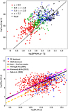 |
Fig. 6. Correlation of AGN and host galaxy properties. The top panel presents the Lbol as a function of SFR. Different symbols and colours correspond to different redshift intervals, as shown in the legend. The solid line indicates the local MBH − M* relation that would be expected from exactly simultaneous evolution of the SMBH and the host galaxy. AGN that lie above this line live in galaxies in which SMBH growth is dominant. AGN that lie below the line are systems in which galaxy growth dominates. The bottom panel shows the distribution of AGN (red circles) and SF (blue circles) dominant systems in the MBH − M* space. The dashed lines are the same as those used in Fig. 4. |
The systems in which the SF is dominant are mainly high-redshift galaxies (median z = 1.85 compared to z = 1.21 for the AGN-dominant systems) and they are in a starburst phase (log sSFR(Gyr−1)> 0.5). They also have similar MBH with their AGN-dominated counterparts at fixed redshift. SF-dominated galaxies also have, on average, a lower log(MBH/M*) ratio (−2.63) compared to AGN-dominated systems (−2.39).
The bottom panel of Fig. 6 presents the MBH − M* relation for the two AGN populations. A Pearson correlation analysis yields an average (over the four redshift intervals) of r = 0.62 ± 0.15 and r = 0.29 ± 0.11 for the SF-dominated and the AGN-dominated galaxies, respectively. This implies a significantly higher correlation between the MBH and M* for the systems in which SF is dominant compared to those in which SMBH growth dominates.
We repeated the same exercise utilising the sample of 69 AGN from the COSMOS and CDFS fields, presented in Sun et al. (2015), and using the values shown in their Table 2. We identified six AGN that are in SF-dominated systems. The median redshift of the two AGN populations is similar (z = 1.32 for systems in which galaxy growth is dominant and z = 1.16 for galaxies in which SMBH growth is dominant). A correlation analysis yields r = 0.41 and r = 0.86 for the AGN-dominated and SF-dominated systems, respectively. The log(MBH/M*) ratio is −2.60 and −2.99 for the galaxies in which SMBH growth dominates and for systems in which galaxy growth dominates, respectively. It is worth mentioning that using Lbol and SFR values from the literature and comparing them with our measurements may hint at systematics (this is also true when comparing our M* and MBH with calculations from the literature), as different methods have been applied for the calculation of these parameters (see e.g., Mountrichas et al. 2021b). Taking into account this caveat and the size of the sample of Sun et al. (2015; in particular the small number of SF-dominated systems it includes), these results confirm the trends we find in our dataset. This could also provide an, alternative, possible explanation for the higher MBH/M* ratio value presented by Setoguchi et al. (2021) and the lack of correlation they found regarding the MBH − M* relation (see the discussion in their Sect. 3.3). Their AGN dataset consists of AGN-dominated galaxies exclusively (see their Fig. 4).
AGN-dominated galaxies appear to have, on average, lower M* compared to their SF-dominated counterparts with similar MBH (bottom panel of Fig. 6). This, in conjunction with their lower correlation between the MBH and M* compared to SF-dominated systems, could suggest that SF growth becomes dominant at a later stage compared to SMBH growth, moving these galaxies rightwards in the MBH − M* plane and in line with local scaling relations. This could also explain the higher MBH/M* ratio of the AGN-dominated systems, in the sense that their M* growth maybe “lags behind” compared to their MBH (or equivalently that their BHs are overweight compared to their stellar mass).
3.5. SMBH mass growth rate versus galaxy stellar mass growth rate
To examine the possible pathways of the AGN in the MBH − M* plane, we calculated the specific SMBH growth rate, defined as sṀ = Ṁ/MBH (Merloni et al. 2010; Sun et al. 2015), where Ṁ is the accretion rate ( , where η = 0.1 is the assumed radiative efficiency of the accretion disc and c is the speed of light) and their specific galaxy stellar mass growth rate, sSFR. The distribution of the AGN used in our study in the sṀ/sSFR–MBH/M* space is presented in the top panel of Fig. 7. Different colours and symbols correspond to different redshift bins. In agreement with Sun et al. (2015), we find a strong anti-correlation between the two parameters at all redshifts spanned by our dataset (r = −0.75 ± 0.12). The horizontal dashed line indicates the sṀ/sSFR = 1, that is when the specific SMBH accretion rate and the sSFR are equal. The vertical dashed line denotes the average MBH/M* ratio value found for our sample.
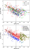 |
Fig. 7. Distribution of AGN in the sṀ/sSFR–MBH/M* space. In the top panel, different colours and symbols correspond to a different redshift bin, as shown in the legend. The bottom panel presents the distribution of SF (blue circles) and AGN (red circles) in the sṀ/sSFR–MBH/M* space. Sources marked with a square are classified as galaxies with overweight SMBHs, while those marked with a triangle are classified as galaxies with underweight SMBHs. The classification is based on the location of the AGN in the MBH − M* plane relative to the line that describes the best fit on our MBH − M* measurements (see text and Fig. 4 for more details). |
The bottom panel of Fig. 7 presents the distribution of systems that are in a SMBH growth-dominant phase (red circles) and those that are in a galaxy growth-dominant phase (blue circles) in the sṀ/sSFR–MBH/M* plane. We also define AGN that lie below the line that describes the best fit on our data in the MBH − M* plane as ‘underweight’ (see black line in Fig. 4), and AGN that lie above this line as ‘overweight’ (including, in both cases, its uncertainty of ∼0.4 dex). These sources are marked with a square (overweight) and a triangle (underweight) in the bottom panel of Fig. 7. We notice that the vast majority of galaxies with underweight SMBHs have sṀ/sSFR > 1, that is to say their specific SMBH mass growth rate is higher than their specific stellar mass growth rate. In other words, their MBH is trying to catch up to their M*. On the opposite side, the vast majority of galaxies with overweight SMBHs have sṀ/sSFR < 1, which implies that the stellar mass growth rate is higher than the SMBH mass growth rate.
4. Summary
We used 687 X-ray luminous (median log [LX,2−10 keV(erg s−1)] = 44.3), BLAGN1, at 0.2 < z < 4.0 (median z ≈ 1.4) that lie in XXL-N. Their bolometric luminosities span nearly three orders of magnitude (44 < log Lbol(erg s−1) < 47), while their BH and stellar masses range from 7.5 < log [MBH (M⊙)] < 9.5 and 10 < log [M*(M⊙)] < 12, respectively. Our goal was to study the co-evolution of the SMBHs and their host galaxies, over a wide redshift range. Our main results can be summarised as follows:
-
The vast majority of the AGN in our dataset are in star-forming systems (Sect. 3.1). Their Eddington ratios range from 0.01 to 1, with a median value of 0.06 (Sect. 3.2).
-
The MBH and M* are correlated. No statistical significant evolution of the MBH/M* ratio is found with redshift up to z = 2. The mean log(MBH/M*)= − 2.44, with a 1σ scatter of 0.61 (Sect. 3.3).
-
Most of the AGN (75%) are in a SMBH growth phase (AGN-dominant phase). In systems in which galaxy mass growth is dominant, the MBH − M* relation is significantly tighter compared to the galaxies that are in an AGN-dominant phase. This could suggest that the growth of BH mass occurs first, while the early stellar mass assembly may not be so efficient (Sect. 3.4).
-
We detect a strong anti-correlation between the MBH/M* ratio and the ratio of the specific SMBH and galaxy mass growth rates. Most of the AGN for which their SMBH is classified as underweighted have sṀ/sSFR > 1, that is their specific SMBH mass growth rate is higher than their specific stellar mass growth rate. The majority of the AGN with overweighted SMBH have sṀ/sSFR < 1, which implies that their stellar masses are catching up to their MBH (Sect. 3.5). The large AGN sample used in this work allowed us to study the co-evolution of SMBHs and their host galaxies, over a wide range of redshift. Additional constraints on this symbiosis can be put by studying the MBH − M* relation as a function of the galaxy’s morphology and local environment.
Acknowledgments
The author acknowledges support by the Agencia Estatal de Investigación, Unidad de Excelencia María de Maeztu, ref. MDM-2017-0765. This project has received funding from the European Union’s Horizon 2020 research and innovation program under grant agreement no 101004168, the XMM2ATHENA project. This research has made use of TOPCAT version 4.8 (Taylor 2005).
References
- Bluck, A. F. L., Piotrowska, J. M., & Maiolino, R. 2023, ApJ, 944, 108 [NASA ADS] [CrossRef] [Google Scholar]
- Boquien, M., Burgarella, D., Roehlly, Y., et al. 2019, A&A, 622, A103 [NASA ADS] [CrossRef] [EDP Sciences] [Google Scholar]
- Bruzual, G., & Charlot, S. 2003, MNRAS, 344, 1000 [NASA ADS] [CrossRef] [Google Scholar]
- Buat, V., Ciesla, L., Boquien, M., Małek, K., & Burgarella, D. 2019, A&A, 632, A79 [NASA ADS] [CrossRef] [EDP Sciences] [Google Scholar]
- Buat, V., Mountrichas, G., Yang, G., et al. 2021, A&A, 654, A93 [NASA ADS] [CrossRef] [EDP Sciences] [Google Scholar]
- Charlot, S., & Fall, S. M. 2000, ApJ, 539, 718 [Google Scholar]
- Ciesla, L., Charmandaris, V., Georgakakis, A., et al. 2015, A&A, 576, 19 [Google Scholar]
- Ciesla, L., Elbaz, D., & Fensch, J. 2017, A&A, 608, A41 [NASA ADS] [CrossRef] [EDP Sciences] [Google Scholar]
- Dale, D. A., Helou, G., Magdis, G. E., et al. 2014, ApJ, 784, 83 [Google Scholar]
- Ferrarese, L., & Merritt, D. 2000, ApJ, 539, 9 [Google Scholar]
- Gebhardt, K., Kormendy, J., Ho, L. C., et al. 2000, ApJ, 543, 5 [Google Scholar]
- Georgakakis, A., & Nandra, K. 2011, MNRAS, 414, 992 [NASA ADS] [CrossRef] [Google Scholar]
- Georgakakis, A., Aird, J., Schulze, A., et al. 2017, MNRAS, 471, 1976 [NASA ADS] [CrossRef] [Google Scholar]
- Gültekin, K., Richstone, D. O., Gebhardt, K., et al. 2009, ApJ, 698, 198 [Google Scholar]
- Häring, N., & Rix, H.-W. 2004, ApJ, 604, L89 [Google Scholar]
- Jahnke, K., Bongiorno, A., Brusa, M., et al. 2009, ApJ, 706, 215 [Google Scholar]
- Komatsu, E., Smith, K. M., Dunkley, J., et al. 2011, ApJS, 192, 18 [Google Scholar]
- Kormendy, J., & Ho, L. C. 2013, ARA&A, 51, 511 [Google Scholar]
- Koutoulidis, L., Mountrichas, G., Georgantopoulos, I., Pouliasis, E., & Plionis, M. 2022, A&A, 658, A35 [NASA ADS] [CrossRef] [EDP Sciences] [Google Scholar]
- Lanzuisi, G., Delvecchio, I., Berta, S., et al. 2017, A&A, 602, 13 [Google Scholar]
- Liu, Z., Merloni, A., Georgakakis, A., et al. 2016, MNRAS, 459, 1602 [Google Scholar]
- Lusso, E., Comastri, A., Simmons, B. D., et al. 2012, MNRAS, 425, 623 [Google Scholar]
- Magorrian, J., Tremaine, S., Richstone, D., et al. 1998, AJ, 115, 2285 [Google Scholar]
- Małek, K., Buat, V., Roehlly, Y., et al. 2018, A&A, 620, A50 [Google Scholar]
- Marconi, A., & Hunt, L. K. 2003, ApJ, 589, L21 [Google Scholar]
- Masoura, V. A., Mountrichas, G., Georgantopoulos, I., et al. 2018, A&A, 618, 31 [Google Scholar]
- Masoura, V. A., Mountrichas, G., Georgantopoulos, I., & Plionis, M. 2021, A&A, 646, A167 [EDP Sciences] [Google Scholar]
- Menzel, M.-L., Merloni, A., Georgakakis, A., et al. 2016, MNRAS, 457, 110 [Google Scholar]
- Merloni, A., Bongiorno, A., Bolzonella, M., et al. 2010, ApJ, 708, 137 [Google Scholar]
- Mountrichas, G., & Shankar, F. 2023, MNRAS, 518, 2088 [Google Scholar]
- Mountrichas, G., Buat, V., Yang, G., et al. 2021a, A&A, 646, A29 [EDP Sciences] [Google Scholar]
- Mountrichas, G., Buat, V., Yang, G., et al. 2021b, A&A, 653, A74 [NASA ADS] [CrossRef] [EDP Sciences] [Google Scholar]
- Mountrichas, G., Buat, V., Yang, G., et al. 2022a, A&A, 663, A130 [NASA ADS] [CrossRef] [EDP Sciences] [Google Scholar]
- Mountrichas, G., Buat, V., Yang, G., et al. 2022b, A&A, 667, A145 [NASA ADS] [CrossRef] [EDP Sciences] [Google Scholar]
- Mountrichas, G., Masoura, V. A., Xilouris, E. M., et al. 2022c, A&A, 661, A108 [NASA ADS] [CrossRef] [EDP Sciences] [Google Scholar]
- Park, D., Woo, J.-H., Bennert, V. N., et al. 2015, ApJ, 799, 164 [NASA ADS] [CrossRef] [Google Scholar]
- Pierre, M., Pacaud, F., Adami, C., et al. 2016, A&A, 592, 1 [Google Scholar]
- Poitevineau, R., Castignani, G., & Combes, F. 2023, A&A, in press, https://doi.org/10.1051/0004-6361/202244560 [Google Scholar]
- Reines, A. E., & Volonteri, M. 2015, ApJ, 813, 82 [NASA ADS] [CrossRef] [Google Scholar]
- Sani, E., Marconi, A., Hunt, L. K., & Risaliti, G. 2011, MNRAS, 413, 1479 [NASA ADS] [CrossRef] [Google Scholar]
- Schramm, M., & Silverman, J. D. 2013, ApJ, 767, 13 [NASA ADS] [CrossRef] [Google Scholar]
- Schreiber, C., Pannella, M., Elbaz, D., et al. 2015, A&A, 575, 29 [Google Scholar]
- Setoguchi, K., Ueda, Y., Toba, Y., & Akiyama, M. 2021, ApJ, 909, 188 [NASA ADS] [CrossRef] [Google Scholar]
- Shankar, F., Bernardi, M., Sheth, R. K., et al. 2016, MNRAS, 460, 3119 [NASA ADS] [CrossRef] [Google Scholar]
- Shankar, F., Bernardi, M., Richardson, K., et al. 2019, MNRAS, 485, 1278 [Google Scholar]
- Shen, Y., & Liu, X. 2012, ApJ, 753, 125 [NASA ADS] [CrossRef] [Google Scholar]
- Shen, Y., Greene, J. E., Strauss, M. A., Richards, G. T., & Schneider, D. P. 2008, ApJ, 680, 169 [Google Scholar]
- Shen, Y., Richards, G. T., Strauss, M. A., et al. 2011, ApJS, 194, 45 [Google Scholar]
- Shen, Y., McBride, C. K., White, M., et al. 2013, ApJ, 778, 98 [Google Scholar]
- Shirley, R., Roehlly, Y., Hurley, P. D., et al. 2019, MNRAS, 490, 634 [Google Scholar]
- Shirley, R., Duncan, K., Varillas, M. C. C., et al. 2021, MNRAS, 507, 129 [NASA ADS] [CrossRef] [Google Scholar]
- Stalevski, M., Fritz, J., Baes, M., Nakos, T., & Popović, L. Č. 2012, MNRAS, 420, 2756 [Google Scholar]
- Stalevski, M., Ricci, C., Ueda, Y., et al. 2016, MNRAS, 458, 2288 [Google Scholar]
- Suh, H., Civano, F., Trakhtenbrot, B., et al. 2020, ApJ, 889, 32 [NASA ADS] [CrossRef] [Google Scholar]
- Sun, M., Trump, J. R., Brandt, W. N., et al. 2015, ApJ, 802, 14 [NASA ADS] [CrossRef] [Google Scholar]
- Sutherland, W., & Saunders, W. 1992, MNRAS, 259, 413 [Google Scholar]
- Taylor, M. B. 2005, in Astronomical Data Analysis Software and Systems XIV, eds. P. Shopbell, M. Britton, & R. Ebert, ASP Conf. Ser., 347, 29 [Google Scholar]
- Tremaine, S., Gebhardt, K., Bender, R., et al. 2002, ApJ, 574, 740 [NASA ADS] [CrossRef] [Google Scholar]
- Trump, J. R., Impey, C. D., Elvis, M., et al. 2009, ApJ, 696, 1195 [NASA ADS] [CrossRef] [Google Scholar]
- Ueda, Y., Hatsukade, B., Kohno, K., et al. 2018, ApJ, 853, 24 [NASA ADS] [CrossRef] [Google Scholar]
- Whitaker, K. E., Franx, M., Leja, J., et al. 2014, ApJ, 795, 104 [NASA ADS] [CrossRef] [Google Scholar]
- Yang, G., Boquien, M., Buat, V., et al. 2020, MNRAS, 491, 740 [Google Scholar]
- Yang, G., Boquien, M., Brandt, W. N., et al. 2022, ApJ, 927, 192 [NASA ADS] [CrossRef] [Google Scholar]
All Figures
|
Fig. 1. SMBH and galaxy properties as a function of redshift. Top panel: MBH vs. redshift. Bottom panel: M* vs. redshift. The dashed horizontal lines show the MBH (top panel) and M* (bottom panel) limits to which our sample is complete up to redshift 2 (vertical lines). For more details, readers can refer to Sect. 3.3. |
| In the text | |
|
Fig. 2. SFR vs. M* of the X-ray AGN in our dataset. Different symbols indicate different redshift intervals, as shown in the legend. The results are colour-coded based on the MBH value. |
| In the text | |
|
Fig. 3. Lbol as a function of MBH. Different symbols and colours correspond to different redshift intervals, as indicated in the legend. The lines correspond to Lbol = LEdd (green long-dashed line), Lbol = 0.1 LEdd (solid black line), and Lbol = 0.01 LEdd (grey short-dashed line). |
| In the text | |
|
Fig. 4. MBH as a function of M*. The top panel shows the distribution of our AGN in the MBH − M* space. Different colours correspond to different redshift bins. The bottom panel shows our results grouped in bins of redshift (red symbols) and M* (green symbols). Median values are presented as well as the 1σ uncertainties (calculated via bootstrap resampling). The labels next to the red points show the median redshift that corresponds to each bin. The solid black line shows the best fit on our measurements. The dashed lines, in both panels, present the best fits from previous studies (see text for more details). |
| In the text | |
|
Fig. 5. MBH − M* ratio as a function of redshift. The top panel shows the values for the total AGN sample. The bottom panel shows the results when we accounted for selection biases (see text for more details). The horizontal dashed black line in both panels indicates the mean MBH − M* ratio value of our dataset. The horizontal long-dashed green line presents the mean MBH − M* ratio value, when selection biases are taken into consideration. |
| In the text | |
|
Fig. 6. Correlation of AGN and host galaxy properties. The top panel presents the Lbol as a function of SFR. Different symbols and colours correspond to different redshift intervals, as shown in the legend. The solid line indicates the local MBH − M* relation that would be expected from exactly simultaneous evolution of the SMBH and the host galaxy. AGN that lie above this line live in galaxies in which SMBH growth is dominant. AGN that lie below the line are systems in which galaxy growth dominates. The bottom panel shows the distribution of AGN (red circles) and SF (blue circles) dominant systems in the MBH − M* space. The dashed lines are the same as those used in Fig. 4. |
| In the text | |
|
Fig. 7. Distribution of AGN in the sṀ/sSFR–MBH/M* space. In the top panel, different colours and symbols correspond to a different redshift bin, as shown in the legend. The bottom panel presents the distribution of SF (blue circles) and AGN (red circles) in the sṀ/sSFR–MBH/M* space. Sources marked with a square are classified as galaxies with overweight SMBHs, while those marked with a triangle are classified as galaxies with underweight SMBHs. The classification is based on the location of the AGN in the MBH − M* plane relative to the line that describes the best fit on our MBH − M* measurements (see text and Fig. 4 for more details). |
| In the text | |
Current usage metrics show cumulative count of Article Views (full-text article views including HTML views, PDF and ePub downloads, according to the available data) and Abstracts Views on Vision4Press platform.
Data correspond to usage on the plateform after 2015. The current usage metrics is available 48-96 hours after online publication and is updated daily on week days.
Initial download of the metrics may take a while.