| Issue |
A&A
Volume 672, April 2023
|
|
|---|---|---|
| Article Number | A109 | |
| Number of page(s) | 12 | |
| Section | Astrophysical processes | |
| DOI | https://doi.org/10.1051/0004-6361/202245505 | |
| Published online | 07 April 2023 | |
Evidence for non-thermal X-ray emission from the double Wolf-Rayet colliding-wind binary Apep
1
Department of Space, Earth and Environment, Chalmers University of Technology, 412 96 Gothenburg, Sweden
e-mail: This email address is being protected from spambots. You need JavaScript enabled to view it.
2
Instituto Argentino de Radioastronomía (CCT La Plata, CONICET; CICPBA; UNLP), C.C.5, (1894) Villa Elisa, Buenos Aires, Argentina
3
Space sciences, Technologies and Astrophysics Research unit – STAR, University of Liège, Quartier Agora, 19c, Allée du 6 Août, B5c, 4000 Sart Tilman, Belgium
4
School of Physics and Astronomy, University of Southampton Highfield Campus, Southampton SO17 1PS, UK
5
Department de Física Quàntica i Astrofísica, Institut de Ciències del Cosmos (ICC), Universitat de Barcelona (IEEC-UB), Martí i Franquès 1, 08028 Barcelona, Spain
6
Joint Institute for VLBI ERIC, Oude Hoogeveensedijk 4, 7991 PD Dwingeloo, The Netherlands
Received:
18
November
2022
Accepted:
15
February
2023
Abstract
Context. Massive colliding-wind binaries (CWBs) can be non-thermal sources. The emission produced in their wind-collision region (WCR) encodes information of both the shock properties and the relativistic electrons accelerated in them. The recently discovered system Apep, a unique massive system hosting two Wolf-Rayet stars, is the most powerful synchrotron radio emitter among the known CWBs. It is an exciting candidate in which to investigate the non-thermal processes associated with stellar wind shocks.
Aims. We intend to break the degeneracy between the relativistic particle population and the magnetic field strength in the WCR of Apep by probing its hard X-ray spectrum, where inverse-Compton (IC) emission is expected to dominate.
Methods. We observed Apep with NuSTAR for 60 ks and combined this with a reanalysis of a deep archival XMM-Newton observation to better constrain the X-ray spectrum. We used a non-thermal emission model to derive physical parameters from the results.
Results. We detect hard X-ray emission consistent with a power-law component from Apep. This is compatible with IC emission produced in the WCR for a magnetic field of ≈105–190 mG, corresponding to a magnetic-to-thermal pressure ratio in the shocks of ≈0.007–0.021, and a fraction of ∼1.5 × 10⁻⁴ of the total wind kinetic power being transferred to relativistic electrons.
Conclusions. The non-thermal emission from a CWB is detected for the first time in radio and at high energies. This allows us to derive the most robust constraints so far for the particle acceleration efficiency and magnetic field intensity in a CWB, reducing the typical uncertainty of a few orders of magnitude to just within a factor of a few. This constitutes an important step forward in our characterisation of the physical properties of CWBs.
Key words: stars: Wolf-Rayet / stars: winds / outflows / radiation mechanisms: non-thermal / acceleration of particles / X-rays: stars
© The Authors 2023
 Open Access article, published by EDP Sciences, under the terms of the Creative Commons Attribution License (https://creativecommons.org/licenses/by/4.0), which permits unrestricted use, distribution, and reproduction in any medium, provided the original work is properly cited.
This article is published in open access under the Subscribe to Open model. This email address is being protected from spambots. You need JavaScript enabled to view it. to support open access publication.
1. Introduction
Colliding-wind binaries (CWBs) are binary systems in which the powerful winds of the massive stars collide. The strong shocks in the wind-collision region (WCR) produce very hot (> 106 K) X-ray emitting plasma. Moreover, they can also accelerate relativistic particles (Eichler & Usov 1993; Benaglia & Romero 2003) and constitute a subset of objects called particle-accelerating CWBs (PACWBs; De Becker & Raucq 2013). The efficiency of this particle-acceleration process is still poorly constrained theoretically and observationally, however. The commonly assumed scenario for particle acceleration in PACWBs is diffusive shock acceleration (DSA; Drury 1983).
Relativistic electrons, which are in general expected to radiate more efficiently than relativistic protons, can up-scatter stellar optical and ultraviolet photons to X-ray or γ-ray emission by the inverse Compton (IC) process. Relativistic electrons can also radiate synchrotron emission in the radio band by interacting with the magnetic fields in the WCR. Many CWBs present non-thermal radio emission (De Becker & Raucq 2013), but this is insufficient to characterise the relativistic electron population and the magnetic field intensity in the emitter without severe partitioning assumptions (De Becker 2018). Meanwhile, detections at hard X-rays and above remain scarce: η-Car has clearly been detected in hard X-rays (Hamaguchi et al. 2018) and γ-rays (Tavani et al. 2009; Reitberger et al. 2015; H.E.S.S. Collaboration 2020; Martí-Devesa & Reimer 2021), while γ2 Vel has recently been confirmed as a γ-ray source (Martí-Devesa et al. 2020), and a tentative detection of non-thermal hard X-rays (E ≲ 18 keV) has been associated with HD 93129A (del Palacio et al. 2020).
The X-ray spectral energy distribution (SED) of a CWB is determined by the thermal and non-thermal radiation components, which depend on the WCR properties, together with the local wind absorption (Pittard & Parkin 2010). The emission from individual stellar winds can only produce soft X-rays at energies ≲1 keV, and the total absorption from most stellar winds and the interstellar medium (ISM) is not relevant above 2 keV. Thus, the SED at energies > 3 keV is determined solely by processes in the WCR. Thermal processes are likely to dominate the SED up to ∼10 keV given the high wind velocities and consequent post-shock temperatures, and thus the non-thermal processes can only be investigated at energies above 10 keV. It is therefore necessary to have a broadband measurement of the X-ray SED to disentangle these two components.
The system Apep is a peculiar case of a massive binary consisting of two Wolf-Rayet stars (Callingham et al. 2019). The stars are separated by more than 100 AU, which allows the stellar winds to accelerate to full speed before collision. Radio observations of this system revealed that it is a very powerful synchrotron source (Callingham et al. 2019), which also establishes it as an efficient particle accelerator. In addition, Marcote et al. (2021) confirmed using very long baseline interferometric observations that this emission rises from the WCR. Further constraints on the radio spectrum by Bloot et al. (2022) allowed del Palacio et al. (2022) to model the source broadband emission in order to infer properties of the stellar winds and predict the SED of the source at high energies. However, these predictions are highly degenerate as it is not possible to disentangle the relativistic particle energy distribution and the magnetic field strength in the WCR, BWCR, from radio data alone (del Palacio et al. 2022). A recent analysis of Fermi-LAT data in γ-rays placed stronger constraints on the high-energy SED of Apep, but was still unable to detect its emission (Martí-Devesa et al. 2023).
In addition, Apep was also observed in soft X-rays on different occasions with XMM-Newton and Chandra. Callingham et al. (2019) analysed this data set and concluded that this source (i) is point-like in X-rays, (ii) is not variable on scales of years, and (iii) has a predominantly thermal spectrum with a significant absorption below 2 keV.
We investigate the hard X-ray spectrum of Apep and search for signatures of a non-thermal IC component, as predicted by del Palacio et al. (2022). The measurement of this component would allow to constrain much better the energy budget in relativistic particles and the magnetic field strength in the WCR. With this purpose, we conducted observations of Apep with NuSTAR, probing its spectrum at energies > 10 keV for the first time. We present the analysis and interpretation of these observations here.
2. Observations and data reduction
2.1. System Apep
The massive binary Apep (2XMM J160050.7−514245) is located at RA = 10h43m57.5s, Dec = −59° 32′51.4″ (J2000). Its orbit is wide, with a separation between the stars of some tens of AU (Han et al. 2020). The primary star is a WN star, and the secondary is a WC star. These stars have very massive and fast winds with kinetic powers of LWN ≈ 1.5 × 1038 erg s−1 and LWC ≈ 4.1 × 1037 erg s−1 (with an uncertainty of ≈30%; see Table 1). This constitutes an abundant energy reservoir to feed emission processes at the WCR. The WCR in Apep is exceptionally luminous: it is the brightest PACWB detected at radio wavelengths (Callingham et al. 2019). A more detailed list of the relevant system parameters is given in Table 1.
Parameters of the WC+WN system Apep.
This source has been observed in X-rays with XMM-Newton and Chandra during 2015–2021. Most of these observations have been analysed previously by Callingham et al. (2019), who showed that the source does not present significant variability in X-rays. We observed this system for the first time with NuSTAR in 2022. In addition, we complemented this with a reanalysis of a deep XMM-Newton observation in order to characterise the X-ray SED of Apep better. We summarise the analysed observations in Table 2 and describe them in more detail in the following subsections.
Summary of the X-ray observations.
2.2. XMM-Newton
Apep is in the field of view of several archival XMM-Newton observations. Of these, Obs. 0742050101 is the deepest (> 100 ks) and therefore the one we chose to analyse. The main drawback of this observation is the large offset from on-axis to the position of Apep, which is 8.8′. The source appears in the PN and MOS2 cameras, and the observation was carried out in full-frame mode. Other details of this observation are summarised in Table 2.
Data processing was performed using the Science Analysis Software SAS v.20.0.0 and the calibration files (CCF) available in August 2022. We used the metatasks emproc and epproc to reduce the data. We then filtered periods of high background or soft proton flares. Standard screening criteria were adopted, namely pattern ≤ 12 for MOS and pattern ≤4 for PN. We determined good time intervals by selecting events with PI> 10 000 and PATTERN==0 and adopting the standard rejection thresholds RATE≤0.35 for MOS2 and RATE≤0.4 for PN. The effective time after filtering is reported in Table 2. These values are 25–30 ks lower than those of Callingham et al. (2019), which suggests that our selection of GTIs was more conservative.
To produce the spectra, the radius of the extraction region was set to 50″, as the source is 8.8′ off axis and therefore the point-spread function (PSF) is larger than for on-axis sources (for which 10–30″ is typically used). The background spectrum was extracted in an elliptical region located on the same chip, in an area devoid of point sources that was selected using the task ebkreg. However, the adopted background region has a negligible impact on the results because the source is very bright. Adequate response matrix files (RMF) and ancillary response files (ARF) were produced using dedicated tasks (rmfgen and arfgen, respectively) for all spectra. On this last point, we note that the standard psfmodel ELLBETA does not work well for MOS2 because Apep is a very bright source and is quite off-axis (8.8′), therefore, we used the psfmodel=EXTENDED option (XMM support, priv. comm.). This correction improved the match between the MOS2 and the PN spectra (a mismatch around 6 keV can be seen in the supplementary information Fig. 4 from Callingham et al. 2019, where the standard ELLBETA model was used for MOS2). Other parameters adopted for the ARF file were extendedsource=no, detmaptype=psf, and applyabsfluxcorr=yes. The last parameter was used to improve the cross-calibration between XMM-Newton and NuSTAR. We finally grouped the spectra using the task ftgrouppha with grouptype=opt.
2.3. NuSTAR
The NuSTAR X-ray observatory was launched in 2012, and its major asset is its unique imaging capacity in hard X-rays. The observatory includes two co-aligned X-ray grazing-incidence telescopes, known as FPMA and FPMB for their focal plane modules, which are comprised of four rectangular solid-state CdZnTe detectors. NuSTAR is capable of observing in the 3–79 keV energy range with an angular resolution of 18″ (half-power diameter of 58″; Harrison et al. 2013).
We observed the massive binary Apep in June 2022 with NuSTAR under program 8020 (PI: del Palacio). The observations were carried out in two 30 ks visits, adding up to roughly 60 ks of exposure time with both cameras. We refer to the observations in each epoch as 2022a and 2022b. We summarise the relevant details of these observations in Table 2.
We reduced the data using Heasoft 6.30.1 and the latest calibration files available in June 2022 (CALDB 4.9.7-0). We used the nupipeline task to create level 2 data products with the options saacalc=2, saamode=optimized, and tentacle=yes to filter high-background epochs. This led to negligible data loss in the 2022a observations and to < 3% data loss in the 2022b observation1. We then used the nuproducts task to create level 3 data products. We extracted the source spectrum from a 55″ region centred on Apep, while the background was extracted from an ellipse located in the same chip, sufficiently far from the source so as to avoid contamination. The selected background region also avoids contamination from the supernova remnant G330.2+1.0, as shown in Fig. 1. Further analysis of the influence of the selected background region is presented in Appendix B. Finally, we binned the spectra using the task ftgrouppha with the option grouptype=opt.
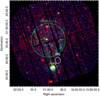 |
Fig. 1. RGB XMM-Newton image of the field of view of Apep (red = 0.3–1.2 keV, green = 1.2–2.5 keV, blue = 2.5–8 keV) from the EPIC-PN detector. We also indicate the position of the supernova remnant G330.2+1.0. |
2.4. XSPEC spectral model
A spectral model is needed to extract physical information from the obtained spectra. Any model adopted should be both physically motivated and simple enough so as to reproduce the data without requiring a very large number of parameters. A spectral model for a PACWB should include an absorption component that can take internal absorption in the stellar winds and external absorption in the ISM into account, a thermal component that is dominated by the WCR emission, and a non-thermal component that is relevant only at E > 10 keV, also produced by the WCR. The thermal emission from CWBs is usually approximated using an apec model (Smith et al. 2001), because it is simple and can reproduce the emission from an optically thin plasma well. Multiple apec components can be used to emulate the temperature gradient along the WCR (e.g., Pittard & Parkin 2010). However, the apec model assumes that electrons and ions are in equilibrium, and the shocks in the WCR can be collisionless under certain conditions, leading to an ionisation that can be out-of-equilibrium. This depends on the relation between two timescales: the dynamical timescale, tdyn, and the electron-ion temperature equalisation timescale, teq. The timescale tdyn depends on the characteristic size of the WCR (∼D) and on the velocity at which the material is advected away (∼v∞), while teq depends on the post-shock temperature and density, and therefore on v∞ and Ṁ. If tdyn < teq, the electrons and ions cannot reach thermal equilibrium through Coulomb interactions before the post-shock plasma is advected away. This condition can be summarised through the parameter  , such that if ζeq < 1, the difference between electron and ion temperatures should be taken into account (Zhekov & Skinner 2000). For long-period binaries, this condition is more likely to be fulfilled, such as in the case of Apep. For the conditions in the shocks of the primary and secondary and using the parameters given in Table 1, we obtain ζ ∼ 0.01 − 0.1. Thus, the use of a non-equilibrium model, such as pshock, is justified in this case, and we explored this possibility as well.
The simplest way to parameterise the non-thermal emission is as a power-law component. We can constrain its spectral index considering that this component is expected to be IC radiation emitted by the same relativistic electron population in the WCR that produces the synchrotron emission observed in the radio band (del Palacio et al. 2022). For a flux density Sν ∝ να in the radio band, the specific photon flux density F ∝ E−Γ in X-rays has a spectral index Γ = −α + 1 (del Palacio et al. 2022). In the case of Apep, a value of α = −0.72 was reported by Callingham et al. (2019), which leads to Γ = 1.72. We note that this value is slightly steeper than the canonical α = −0.5 (Γ = 1.5) expected to arise from electrons accelerated by DSA in high Mach number shocks under the test-particle assumption. Nonetheless, this trend of steeper spectra is also seen in supernova remnants and can be related to the back-reaction of cosmic rays in the shocks (e.g., Drury 1983; Gabici et al. 2019).
Finally, the emitted X-ray radiation can be absorbed intrinsically in the source and externally in the ISM. In XSPEC, the standard model used to calculate the ISM absorption is TBabs. The value of the NH column can be taken from HI4PI Collaboration (2016)2. For Apep, the value retrieved is NH = 1.63 × 1022 cm−2. Additional intrinsic absorption (mostly by the stellar winds) can be included using a phabs model. Throughout this work, the confidence intervals are obtained using the error command in XSPEC and are given at a 1 σ level unless stated otherwise.
3. Results
3.1. XMM-Newton
In Fig. 1 we show an RGB exposure-corrected image of the field of view of XMM-Newton. We also show the source and background extraction regions.
To fit the XMM-Newton spectra, we first considered a model of the form constant*TBabs*apec, with abundances set to Wilms (Wilms et al. 2000), as done by Callingham et al. (2019). The normalisation constant was set to unity for PN and then fitted to MOS2, from which we obtained C = 1.06 ± 0.01. We show the fitted spectra in Fig. 2. In general, we found results that were very similar to those of Callingham et al. (2019) (kT ≈ 5.1 keV, NH ≈ 2.7 × 1022 cm−2, abundance A ≈ 0.5, and observed flux F0.3 − 10 keV ≈ 8 × 10⁻¹² erg s−1 cm−2), despite the differences in the data reduction (Sect. 2.2). Nonetheless, the goodness of the fit was quite poor, yielding high structured residuals around 1–2.5 keV at energies coincident with known Si and S transitions (Fig. 2) and a C-Stat 439.0/224. This motivated us to search for a better model.
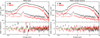 |
Fig. 2. Apep XMM-Newton spectra in the 0.3–10 keV energy range. In the left panel, the fitted model is TBabs*apec, and in the right panel, it is TBabs*vphabs*vpshock. The latter model is preferred as it leads to lower residuals between 1 and 2.5 keV. |
As discussed in Sect. 2.4, adopting a pshock model instead of an apec is physically justified in the case of Apep. The use of a pshock model required only one additional free parameter, namely the upper limit on the ionisation timescale (τu), and it improved the quality of the fit significantly (C-Stat 311.5/223). We note that this affected only the low-energy portion of the spectrum, in particular, by improving the ratios in the Si and S lines. This suggests that ionisation was indeed out of equilibrium, and is also consistent with the value obtained of τu < 1012 s cm3. However, this had a completely negligible (∼1%) impact on the spectra at energies above 3 keV. Further improvement can be achieved by setting variable abundances: although Callingham et al. (2019) claimed that using a vapec model did not improve the fit significantly, we found that a vpshock model can indeed introduce a significant improvement, reaching C-Stat 270.9/220. This is also shown in Fig. 2, which highlights the lower residuals retrieved in the 1–2.5 keV energy range with this model. When fitting the individual abundances, we obtained a similar value for Fe as for A, indicating that this element dominates the value of A for fixed relative abundances. A few elements presented different abundances (mainly Ne), while others, such as C and N, were not constrained by the data and were left fixed to one. Finally, as the stellar winds are expected to contribute significantly to the (photoelectric) absorption, we changed the absorption model to TBabs*vphabs, fixing NH = 1.63 × 1022 cm−2 for the TBabs component (Sect. 2.4) and fixed the abundances of the vphabs to those of the vpshock model. This improved the fit slightly (C-Stat 268.4/220) without adding additional free parameters. It is therefore our preferred model for the XMM-Newton data. In Table 3 we present all the fitted parameters for the most relevant models in detail, including the data from NuSTAR, as discussed in the next section. When the PN camera is taken as reference, the observed flux in the 0.3–10 keV energy range is F0.3 − 10 keV, obs = (7.92 ± 0.10)×10−12 erg s−1 cm−2, the ISM-unabsorbed flux is F0.3 − 10 keV, unabs = (9.69 ± 0.05)×10−12 erg s−1 cm−2, and the unabsorbed flux from the vpshock component alone is F0.3 − 10 keV, vpshock = (1.89 ± 0.04)×10−11 erg s−1 cm−2.
Results of the fitting of NuSTAR and XMM-Newton spectra of Apep using different models.
3.2. NuSTAR
In Fig. 3 we present an image in the 3–20 keV energy range (PI channels 35–460) with NuSTAR for each observing epoch and camera. Apep is clearly detected, and no other bright sources appear in the field. We note straylight in the FPMB observations, although this is not problematic because Apep is far away from it. In Fig. 3 we also show the selected source and background extraction regions.
 |
Fig. 3. NuSTAR image in the 3–20 keV energy range for the 2022a (left panels) and 2022b observations (right panels). For each epoch and camera, we show the selected source and background extraction regions. Straylight can be seen at the bottom right corner of the FPMB observations. |
The spectra we obtained for each epoch and camera are shown together in Fig. A.1 for comparison. All observations reveal a very similar spectrum in which the source is detected above the background up to ≳20 keV. We calculated the integrated source flux in the 3–10 keV and 10–25 keV energy ranges for each observation for a quantitative comparison3. In all cases, the fluxes differ by less than 10% and are compatible within the 1σ level. We checked whether it was possible to combine the data from the two observations to increase the signal-to-noise ratio. To do this, we co-added the spectra of both cameras for each epoch using the addspec task with the options qaddrmf=yes qsubback=yes and the default value bexpscale=1000. We repeated the calculation of the integrated fluxes and obtained variations below 2% (< 1σ difference), indicating that they are perfectly compatible. This is to be expected considering that the observations were taken very close in time to each other.
We then co-added the spectra of both epochs for each camera to determine whether FPMA and FPMB showed systematic differences. We obtained that the FPMA fluxes in the 3–10 keV were slightly (≈5%) higher than for FPMB (with a 1σ significance), while in the 10–25 keV range, the fluxes between the two cameras match up to 2%, and this difference is less significant (< 1σ). This is within the calibration uncertainties of the instrument (Madsen et al. 2015, 2022). From these tests, we concluded that the two observations are compatible, but with a small difference between the cameras. We therefore decided to work with both NuSTAR observations co-added for each camera separately to improve the signal-to-noise ratio at the highest energies while preventing cross-calibration errors to introduce further errors to the fitting of the spectra. In Fig. A.1 we show the spectrum obtained for the combined observations. In this case, the statistics are improved, as expected, and the source is brighter than the background up to ∼25 keV. In the fitting, we included data up to 35 keV as there is valuable spectral information between 25–35 keV, and we used Cash statistics in XSPEC to properly handle the low number of counts in this energy range.
We tried fitting different models to the NuSTAR spectra. The main conclusion is that these spectra are not sensitive to the adopted absorption model (as the absorption at energies > 3 keV is negligible) nor to the specifics of the emission model (as the information from emission lines is poor). Thus, we simply adopted the same model as we used to fit the XMM-Newton spectra, constant*TBabs*vphabs*vpshock, leaving the abundances and absorption fixed (but allowing temperature and normalisation to vary). Refitting the spectrum allowed us to obtain the normalisation constant between FPMA (taken as unity) and FPMB, C = 0.958 ± 0.015. A high-temperature (k T ∼ 5 keV) thermal component naturally extends to energies above 10 keV and can explain most of the emission detected with NuSTAR. In Fig. 4 we show the spectra and the residuals. However, the residuals at energies > 20 keV become increasingly high, with deviations between 3–7 σ. These deviations can be attributed to the putative non-thermal component. We therefore included an additional power-law (po) component. In this way, we obtained a significantly improved fit, as can be seen in the residuals in the right panel of Fig. 4, as well as in the lower C-stat value (which decreased from 237.5/182 to 203.1/181). For completeness, we note that an additional high-temperature vpshock component with kT > 10 keV also leads to a similar improvement in the fit (although with higher residuals at energies ∼30 keV). However, these high temperatures are not expected in CWB shocks, while a non-thermal component should arise naturally given the (already established in the radio band) presence of non-thermal particles. Thus, the main conclusion here is that the NuSTAR data by themselves strongly support the existence of an additional high-energy component, which we interpret hereon as a (non-thermal) power-law component. More robust results can be derived by consistently including the data from XMM-Newton, which we address in the next section.
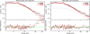 |
Fig. 4. Apep NuSTAR spectra in the 3–35 keV energy range from co-adding the observations for each camera separately. In the left panel, the fitted model is TBabs*vphabs*vpshock, and in the right panel, an additional power-law component is added as TBabs*vphabs*(vpshock+po). |
3.3. Joint analysis
The previous fitting to each instrument separately allowed us to understand the behaviour of the X-ray spectra and to determine which observations are more sensitive to each component. Namely, the XMM-Newton data allow us to better constrain the absorption and thermal emission models, whereas the NuSTAR data are sensitive to the putative high-energy non-thermal component. We now present a joint analysis of the whole data set for the same models as before. In general, we allowed for a different normalisation constant between the different instruments4 and tied the remaining physical parameters.
In Fig. 5 we show the spectra and the combined fitting for two different models, and in Table 3, we detail the fitted parameters for the most relevant models. The TBabs*apec model, used previously by Callingham et al. (2019), fails to reproduce the spectra measured by both XMM-Newton and NuSTAR. The TBabs*vphabs*vpshock model satisfactorily fits the XMM-Newton spectra, but it struggles with the NuSTAR spectra at energies above 20 keV (Fig. 5). Finally, the TBabs*vphabs*(vpshock+po) model can fit all the spectra simultaneously. In this case, the C-stat diminished from 510.5/402 to 491.2/401. The improvement is more significant for NuSTAR at the expense of a slightly poorer fit for XMM-Newton (Table 3). We further quantified the significance of the power-law component using the task simftest in XSPEC. We ran 11 000 simulations and obtained a probability < 0.01% that the data are consistent with a model without the power-law component, which corresponds to a significance > 3.91σ. We also note that the inclusion of the power-law component has little effect on the overall fit, mainly by diminishing the temperature of the thermal component slightly (from ≈5.3 to ≈4.9 keV; Table 3). We finally introduced a cflux component to calculate the total flux in the 10–30 keV band, F10 − 30 keV = (1.99 ± 0.11)×10−12 erg s−1 cm−2, and the flux coming from the power-law component alone,  erg s−1 cm−2.
 |
Fig. 5. Apep unfolded X-ray spectra in the 1–35 keV energy range with XMM-Newton and NuSTAR. The fitted models are constant*TBabs*vphabs*vpshock (left panel) and constant*TBabs*vphabs*(vpshock+po) (right panel). The spectra was rebinned for clarity. The fitted parameters are given in Table 3. |
We note that the flux of the power-law component is susceptible to the background extraction region chosen for NuSTAR, although its presence is always statistically favoured. A detailed exploration of different background regions and the caveats in their selection are given in Appendix B, together with a complementary analysis of the background using nuskybgd Wik et al. (2014). The latter yields a flux of  erg s−1 cm−2 for the power-law component, which is consistent with the previous result within 1σ.
We also corroborated whether the value adopted for the power-law index had a significant impact on the results. For Γ in the range 1.6–1.8, F10 − 30 keV varied only slightly (∼2%), by much less than 1σ. Thus, the value adopted for Γ does not affect the integrated flux in the hard X-ray band. We conclude that the presence of a power-law component is robust, and that its flux can only be measured with a rather high uncertainty.
4. Discussion
The main result from our spectral analysis is the detection of hard X-ray emission consistent with a power-law component with a flux of  erg s−1 cm−2. We also constrained the thermal emission from the WCR much better. Previous estimates of the plasma temperature by Callingham et al. (2019) were highly uncertain, spanning a range kT ∼ 4.7–6.3 keV (for the particular XMM-Newton observation that we also analysed, they obtained kT ∼ 4.9–5.3 keV). By means of a more careful analysis of the XMM-Newton observations, combined with the unique information provided by NuSTAR above 10 keV, we constrain it to kT ≈ 4.85–5.07 keV.
We now focus on the interpretation of the non-thermal component. To be more conservative, in what follows, we consider additional sources of errors in the flux values, both statistical and systematic. For example, a 10% systematic error due to absolute calibration uncertainties is estimated for NuSTAR (Harrison et al. 2013). The retrieved flux additionally depends on the chosen background region, as shown in Appendix B. Based on this, we adopt a less strongly constrained flux of F10 − 30 keV = (2–6)×10−13 erg s−1 cm−2 in our analysis, which is slightly broader than the 90% confidence interval obtained from the analysis with nuskybgd in Appendix B (F10 − 30 keV ∼ (2.3–5.6)×10−13 erg s−1 cm−2).
4.1. Modelling the hard X-ray emission
According to del Palacio et al. (2022), the hard X-ray emission should arise from IC scattering of stellar photons by relativistic electrons in the WCR. These same electrons are also expected to produce the non-thermal (synchrotron) emission observed in the radio band (Callingham et al. 2019; Marcote et al. 2021; Bloot et al. 2022). In order to relate the observed fluxes with the particle acceleration in the shocks, we need to take into account that only a fraction of the wind kinetic power can be converted into relativistic particles in the shocks, that this energy is distributed in electrons and protons, and that each of this particle species radiates only a fraction of their energy at any given frequency range (e.g., De Becker & Raucq 2013).
To model this emission, we therefore used a code based on the non-thermal emission model presented in del Palacio et al. (2016) with the system parameters listed in Table 1. The model solves for the acceleration and transport of relativistic particles for both shocks in the WCR (one for each stellar wind). These relativistic particles radiate by different processes (synchrotron, IC, and p − p collisions), and this radiation is mitigated by absorption processes in the stellar winds or radiation fields. The model has two free parameters that determine the leptonic emission: the ratio of the magnetic field pressure to thermal pressure in the WCR, ηB, and the fraction of the available power at the shocks that is converted into relativistic electrons, fNT, e. The available power for particle acceleration is the wind kinetic power injected perpendicularly into the WCR shocks. Denoting this power by Linj, ⊥ and the total wind kinetic power of a star by  , we can write Linj, ⊥ = ϵLw, with ϵWN = 8% and ϵWC = 18% for the system Apep. Here, the value of ϵ depends on the geometry of the WCR, which is governed by the value of the wind-momentum rate ratio η, and is calculated numerically in the model. Further details of the model are described in Appendix C.
It is possible to tie the two free parameters, fNT, e and ηB, by modelling the observed synchrotron component (del Palacio et al. 2016). In this case, the relation is fNT, eηB = constant (del Palacio et al. 2020). However, it is not possible to break the degeneracy between these two parameters from radio data alone. Fortunately, this can be solved when observations in hard X-rays measure the flux from the IC component, which only depends on fNT, e as FIC ∝ fNT, e (del Palacio et al. 2020). When fNT, e is derived from the measured hard X-ray flux, we can obtain ηB by fitting the synchrotron emission to the observed radio flux of ≈ 120 mJy at 2 GHz (Callingham et al. 2019). In Fig. 6 we show the SEDs fitted using this procedure. In addition, for a given value of ηB, we can calculate the magnetic field in the apex of the WCR, BWCR.
 |
Fig. 6. Modelled broadband non-thermal SED of Apep. We show SEDs for the two extreme combinations of parameters that are compatible with the hard X-ray emission component detected with NuSTAR (this work) and with the ATCA radio data (Callingham et al. 2019). Dashed lines show the synchrotron component, dot-dashed lines show the IC component, dotted lines show the p-p component, and solid lines show the total SED. We also show the Fermi-LAT upper limits from Martí-Devesa et al. (2023) and the sensitivity curve for CTA (Funk et al. 2013). |
Previous estimates by del Palacio et al. (2022) based only on the synchrotron emission from the source had an uncertaintly of more than one order of magnitude in fNT, e, namely fNT, e ≈ (0.11–2.7)×10−3. Our new estimates based on the NuSTAR detection yield a very well-constrained value with an uncertainty smaller than a factor of two, fNT, e ≈ (0.7–2)×10−3. This means that roughly 1.5 × 10⁻⁴ of the total wind kinetic power is converted into relativistic electron acceleration. Moreover, the magnetic field in the WCR was also poorly constrained by del Palacio et al. (2022) to BWCR ≈ 70–400 mG (ηB = (3–100)×10−3), while now, we constrained it to BWCR ≈ 105–190 mG (ηB = 0.007–0.021). This translates into a ratio of the energy density in relativistic electrons and the magnetic field of Ue/UB ≈ 0.02–0.2. For reasonable values of a ratio of the power injected in electrons and protons of Ke, p < 0.1, this leads to a magnetic field in subequipartition with the non-thermal particles, which in turn supports the possibility that relativistic protons drive the magnetic field amplification (Bell 2004).
These values can be compared with those found for the O+O binary HD 93129A during its periastron passage (del Palacio et al. 2020), fNT, e ≈ 6 × 10⁻³ and ηB ∼ 0.02 (BWCR ≈ 0.5 G). Comparisons with other systems are complicated because the detection of a PACWB in both radio and high energies is unique. Nonetheless, we can comment on the PACWB η-Car, for which non-thermal hard X-rays were also detected with a power-law index Γ ∼ 1.65 (although poorly constrained; Hamaguchi et al. 2018). Other systems studied by De Becker (2018), based on radio observations and equipartition assumptions between relativistic particles and magnetic fields, yielded that the fraction of the wind kinetic power converted into relativistic electrons is ∼10−4–10−6 for Cyg OB2 #8a, ∼10−7–10−9 for WR 140, and ∼10−5–10−7 for HD 167971. Compared with the value obtained here for Apep (1.5 × 10⁻⁴), it is clear that this system is a much more efficient electron accelerator. This is consistent with the fact that this binary is the brightest synchrotron-emitting PACWB. We also tried to compare the values of ηB with those derived from De Becker (2018). These values are 10−7 for WR 140, 2 × 10⁻⁴ for Cyg OB2 #8a, and 5 × 10⁻⁵ for HD 167971, but their uncertainty spans two to three orders of magnitude, so that all we can say is that our value of ηB ≈ 10−2 is exceptionally well constrained. In addition, Pittard et al. (2021) fitted the radio SED of the system WR 146 to derive a magnetic field compatible with ηB ≈ 10−3, although these authors required a very high particle efficiency in return (fNT ≈ 0.3).
One last parameter we were able to derive from our results is the surface magnetic field of the stars. To do this, we assumed a toroidal stellar magnetic field that drops as r−1 and is adiabatically compressed in the WCR shocks, and a stellar rotation velocity of Vrot ∼ 0.1v∞ (del Palacio et al. 2016, and references therein). Under these assumptions, we obtain values of the surface stellar magnetic fields in the ranges BWN = 650–1100 G and BWC = 280–490 G. Nonetheless, it is possible that magnetic field amplification processes take place in the WCR shocks (e.g., Bell 2004; Pittard et al. 2021). In this case, the aforementioned values should be interpreted as upper limits for the stellar magnetic fields.
4.2. Predictions of γ-ray emission
The previous estimates of the power in relativistic electrons also allowed us to compute the expected IC luminosity in the γ-ray domain. In Fig. 6 we show the modelled broadband SED extending to γ-ray energies, together with characteristic sensitivity thresholds of γ-ray observatories. We first focus on the 0.1–100 GeV energy range, which can be tested with observations with the Fermi-LAT instrument. The γ-ray luminosity in this case is F0.1 − 100 GeV = (1.9 ± 0.9)×10−12 erg s−1 cm−2, although it can be higher when a hadronic component is included (e.g., Ke, p = 0.04 yields to a total flux of F0.1 − 100 GeV = (2.0 ± 1.5)×10−12 erg s−1 cm−2). These values are mostly consistent with a non-detection of this source with Fermi-LAT at a level of F0.1 − 100 GeV ∼ (1–2)×10−12 erg s−1 cm−2 (Martí-Devesa et al. 2023). The small tension between the higher fluxes predicted for the lower magnetic field scenarios might suggest that the higher magnetic field scenarios are to be preferred (Fig. 4). Nonetheless, this tension can also be attributed to even small uncertainties in the particle energy distribution that lead to a significant difference in the predicted γ-ray fluxes. Assuming that the injected electron energy distribution is slightly harder, p = 2.3 (equivalently, Γ = 1.65), we obtain F0.1 − 100 GeV ∼ 4.2 × 10⁻¹² erg s−1 cm−2, while a slightly steeper distribution, p = 2.55 (Γ = 1.77), yields an IC emission of F0.1 − 100 GeV ∼ (1.0 ± 0.7)×10−12 erg s−1 cm−2. Thus, a hardening of the electron energy distribution is strongly disfavoured as it would overpredict the γ-ray luminosity. Moreover, we conclude that the source is either almost detected by Fermi or that a non-detection with deeper sensitivity (F0.1 − 100 GeV < 10−12 erg s−1 cm−2) would mean that the SED softens at energies above hard X-rays, which in turn would require a softening in the electron energy distribution at energies Ee > 100 MeV.
Finally, we address the prospects for a detection of TeV emission from Apep. We predict an IC flux of FTeV ∼ 1.8 × 10⁻¹⁴ erg s−1 cm−2 in the 0.1–10 TeV energy range, although the poorly constrained hadronic component is likely dominant (del Palacio et al. 2022): When we assume Ke, p = 0.04, the predicted total flux (p − p + IC) is FTeV ∼ 8 × 10⁻¹⁴ erg s−1 cm−2. Moreover, small variations in the spectral index of the particle energy distribution (p = 2.3–2.5) can lead to significantly different TeV fluxes, FTeV ∼ (0.3–18)×10−14 erg s−1 cm−2. Only the higher fluxes might be detectable by the Cherenkov Telescope Array (CTA; Funk et al. 2013), but they are already disfavoured in view of the lack of detections of GeV emission. Thus, the TeV emission from Apep seems too faint to be detected with current and upcoming TeV observatories.
5. Conclusions
We presented the first hard X-ray view of the PACWB Apep. This system is the brightest synchrotron source of the known PACWBs. The NuSTAR spectrum revealed strong evidence of a power-law component, consistent with the predicted IC emission produced by relativistic electrons in the WCR. The detection of this non-thermal high-energy emission from a system that also presents non-thermal emission in the radio band represents an observational breakthrough in the study of PACWBs. In particular, it has allowed us to place the tightest constraints on the magnetic field and electron acceleration efficiency in the WCR of a PACWB. We also predict that Apep is close to being detected at γ-rays with Fermi unless the electron energy distribution softens at energies > 100 MeV.
We highlight the importance of multi-wavelength observations for improving our understanding of PACWBs. Unfortunately, the high-energy emission from these systems is rather weak and difficult to detect, but at least for the brightest sources, observations in the hard X-ray and high-energy γ-rays bands have proven to be successful, paving the way for moving forward in the research of PACWBs.
The differences in absolute flux calibration between XMM-Newton and NuSTAR can be of 5–15% (Madsen et al. 2017).
We note that the apparently very low background error bars returned by the addspec task are appropriate (FTOOLS helpdesk, priv. comm.).
Acknowledgments
We would like to thank the referee for providing useful feedback that helped us to improve the manuscript. This work was carried out in the framework of the PANTERA-Stars (https://www.astro.uliege.be/~debecker/pantera/) initiative. FG is CONICET Researcher and was supported by PIP 0113 (CONICET), PICT-2017-2865 (ANPCyT), and PIBAA 1275 (CONICET). FG was also supported by grant PID2019-105510GB-C32/AEI/10.13039/501100011033 from the Agencia Estatal de Investigación of the Spanish Ministerio de Ciencia, Innovación y Universidades, and by Consejería de Economía, Innovación, Ciencia y Empleo of Junta de Andalucía as research group FQM-322, as well as FEDER funds. D.A. acknowledges support from the Royal Society. V.B.-R. is Correspondent Researcher of CONICET, Argentina, at the IAR. G.E.R. was supported by grant PIP 11220200100554CO (CONICET). This work received financial support from the State Agency for Research of the Spanish Ministry of Science and Innovation under grant PID2019-105510GB-C31/AEI/10.13039/501100011033 and through the “Unit of Excellence María de Maeztu 2020-2023” award to the Institute of Cosmos Sciences (CEX2019-000918-M). This work also made use of the softwares ds9 (Joye & Mandel 2003) and Matplotlib (Hunter 2007).
References
- Bell, A. R. 2004, MNRAS, 353, 550 [Google Scholar]
- Benaglia, P., & Romero, G. E. 2003, A&A, 399, 1121 [NASA ADS] [CrossRef] [EDP Sciences] [Google Scholar]
- Bloot, S., Callingham, J. R., & Marcote, B. 2022, MNRAS, 509, 475 [Google Scholar]
- Callingham, J. R., Tuthill, P. G., Pope, B. J. S., et al. 2019, Nat. Astron., 3, 82 [Google Scholar]
- Callingham, J. R., Crowther, P. A., Williams, P. M., et al. 2020, MNRAS, 495, 3323 [NASA ADS] [CrossRef] [Google Scholar]
- Cappa, C., Goss, W. M., & van der Hucht, K. A. 2004, AJ, 127, 2885 [NASA ADS] [CrossRef] [Google Scholar]
- Crowther, P. A. 2007, ARA&A, 45, 177 [Google Scholar]
- De Becker, M. 2018, A&A, 620, A144 [NASA ADS] [CrossRef] [EDP Sciences] [Google Scholar]
- De Becker, M., & Raucq, F. 2013, A&A, 558, A28 [NASA ADS] [CrossRef] [EDP Sciences] [Google Scholar]
- del Palacio, S., Bosch-Ramon, V., Romero, G. E., & Benaglia, P. 2016, A&A, 591, A139 [NASA ADS] [CrossRef] [EDP Sciences] [Google Scholar]
- del Palacio, S., García, F., Altamirano, D., et al. 2020, MNRAS, 494, 6043 [NASA ADS] [CrossRef] [Google Scholar]
- del Palacio, S., Benaglia, P., De Becker, M., Bosch-Ramon, V., & Romero, G. E. 2022, PASA, 39, e004 [NASA ADS] [CrossRef] [Google Scholar]
- Drury, L. O. 1983, Rep. Progr. Phys., 46, 973 [Google Scholar]
- Eichler, D., & Usov, V. 1993, ApJ, 402, 271 [Google Scholar]
- Funk, S., Hinton, J. A., & CTA Consortium 2013, Astropart. Phys., 43, 348 [NASA ADS] [CrossRef] [Google Scholar]
- Gabici, S., Evoli, C., Gaggero, D., et al. 2019, Int. J. Mod. Phys. D, 28, 1930022 [CrossRef] [Google Scholar]
- H.E.S.S. Collaboration (Abdalla, H., et al.) 2020, A&A, 635, A167 [NASA ADS] [CrossRef] [EDP Sciences] [Google Scholar]
- Hamaguchi, K., Corcoran, M. F., Pittard, J. M., et al. 2018, Nat. Astron., 2, 731 [CrossRef] [Google Scholar]
- Hamann, W. R., Gräfener, G., Liermann, A., et al. 2019, A&A, 625, A57 [NASA ADS] [CrossRef] [EDP Sciences] [Google Scholar]
- Han, Y., Tuthill, P. G., Lau, R. M., et al. 2020, MNRAS, 498, 5604 [NASA ADS] [CrossRef] [Google Scholar]
- Harrison, F. A., Craig, W. W., Christensen, F. E., et al. 2013, ApJ, 770, 103 [Google Scholar]
- HI4PI Collaboration (Ben Bekhti, N., et al.) 2016, A&A, 594, A116 [NASA ADS] [CrossRef] [EDP Sciences] [Google Scholar]
- Hunter, J. D. 2007, Comput. Sci. Eng., 9, 90 [NASA ADS] [CrossRef] [Google Scholar]
- Joye, W. A., & Mandel, E. 2003, in Astronomical Data Analysis Software and Systems XII, eds. H. E. Payne, R. I. Jedrzejewski, & R. N. Hook, ASP Conf. Ser., 295, 489 [NASA ADS] [Google Scholar]
- Leitherer, C., Chapman, J. M., & Koribalski, B. 1995, ApJ, 450, 289 [NASA ADS] [CrossRef] [Google Scholar]
- Madsen, K. K., Harrison, F. A., Markwardt, C. B., et al. 2015, ApJS, 220, 8 [Google Scholar]
- Madsen, K. K., Beardmore, A. P., Forster, K., et al. 2017, AJ, 153, 2 [Google Scholar]
- Madsen, K. K., Forster, K., Grefenstette, B., Harrison, F. A., & Miyasaka, H. 2022, J. Astron. Telesc. Instrum. Syst., 8, 034003 [NASA ADS] [CrossRef] [Google Scholar]
- Marcote, B., Callingham, J. R., De Becker, M., et al. 2021, MNRAS, 501, 2478 [NASA ADS] [CrossRef] [Google Scholar]
- Martí-Devesa, G., & Reimer, O. 2021, A&A, 654, A44 [NASA ADS] [CrossRef] [EDP Sciences] [Google Scholar]
- Martí-Devesa, G., Reimer, O., Li, J., & Torres, D. F. 2020, A&A, 635, A141 [Google Scholar]
- Martí-Devesa, G., Reimer, O., & Reimer, A. 2023, A&A, 670, L6 [NASA ADS] [CrossRef] [EDP Sciences] [Google Scholar]
- Martinez, J. R., del Palacio, S., Bosch-Ramon, V., & Romero, G. E. 2022, A&A, 661, A102 [NASA ADS] [CrossRef] [EDP Sciences] [Google Scholar]
- Merten, L., Becker Tjus, J., Eichmann, B., & Dettmar, R.-J. 2017, Astropart. Phys., 90, 75 [NASA ADS] [CrossRef] [Google Scholar]
- Park, S., Kargaltsev, O., Pavlov, G. G., et al. 2009, ApJ, 695, 431 [NASA ADS] [CrossRef] [Google Scholar]
- Pittard, J. M., & Parkin, E. R. 2010, MNRAS, 403, 1657 [NASA ADS] [CrossRef] [Google Scholar]
- Pittard, J. M., Romero, G. E., & Vila, G. S. 2021, MNRAS, 504, 4204 [NASA ADS] [CrossRef] [Google Scholar]
- Reitberger, K., Reimer, A., Reimer, O., & Takahashi, H. 2015, A&A, 577, A100 [NASA ADS] [CrossRef] [EDP Sciences] [Google Scholar]
- Sander, A. A. C., Hamann, W. R., Todt, H., et al. 2019, A&A, 621, A92 [NASA ADS] [CrossRef] [EDP Sciences] [Google Scholar]
- Smith, R. K., Brickhouse, N. S., Liedahl, D. A., & Raymond, J. C. 2001, ApJ, 556, L91 [Google Scholar]
- Tavani, M., Sabatini, S., Pian, E., et al. 2009, ApJ, 698, L142 [NASA ADS] [CrossRef] [Google Scholar]
- Wik, D. R., Hornstrup, A., Molendi, S., et al. 2014, ApJ, 792, 48 [NASA ADS] [CrossRef] [Google Scholar]
- Wilms, J., Allen, A., & McCray, R. 2000, ApJ, 542, 914 [Google Scholar]
- Zhekov, S. A., & Skinner, S. L. 2000, ApJ, 538, 808 [Google Scholar]
Appendix A: NuSTAR co-added data
In the top panel of Fig. A.1, we show the NuSTAR spectra for the two NuSTAR observations and for the two cameras independently. As detailed in Sect. 2.3, we co-added the spectra of both epochs for each camera to determine any systematic difference between FPMA and FPMB. The result is shown in the middle panel of Fig. A.15. Even though the two cameras are compatible, there is a small difference between them at energies < 10 keV, and for this reason, they were not combined in the detailed analysis carried out in Sect. 3. Nonetheless, we also explored the result of co-adding the two cameras in order to improve the signal-to-noise ratio at the highest energies (neglecting the error introduced at lower energies). The result is shown in the bottom panel of Fig. A.1. This last spectrum has improved statistics at energies > 20 keV and allows us to better see the shape of the SED by eye. Additionally, the fitting of this co-added data-set retrieved results for the best-fitting parameters that are fully compatible with those obtained in Sect. 2.3 without co-adding the cameras.
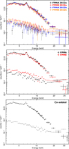 |
Fig. A.1. Apep NuSTAR spectra in the 3–35 keV energy range. The spectra were further rebinned in XSPEC for clarity. The source spectrum is shown with crosses and the background spectrum with open circles. Top panel: Spectra for the 2022a and 2022b observations showing each camera separately. Middle panel: Spectrum from the co-added observations from both epochs (for each camera separately). Bottom panel: Spectrum from the co-added observations (both epochs, both cameras). |
Appendix B: NuSTAR background
As discussed in Sect. 3, the selection of the background extraction region can have a mild impact on the high-energy spectrum of Apep derived with NuSTAR. We explore this in more detail to ensure that our results are robust.
In Fig. B.1 (top panel) we show an image in the 20–35 keV range of the Apep field of view for the first observation with FPMB, in which Apep is clearly detected above the local background. We note that other high-intensity background regions appear in this image, but they are not consistent in the observations and FPM cameras; in contrast, the count excess at the position of Apep is confirmed in all cases, which strongly supports its detection. In this image, we also indicate the different background regions analysed here, labelled bkg1–bkg5. The corresponding background-subtracted spectra of Apep and the background spectra are also shown in Fig. B.1 (bottom panel).
-
bkg1: This elliptical region is our preferred choice as it is within the same chip as the source, which is the usual recommendation for analysing NuSTAR data, and it is sufficiently far from Apep and other sources in the field. This background region leads to a power-law component with a significance of > 3.91σ (< 0.01% of a serendipitous detection) with a flux of
 erg s−1 cm−2.
 -
bkg2: An annulus region centred on the position of Apep and with inner radius of 135″and outer radius of 170″. We note that ≈90% of the photons from Apep should be contained within a 130″from the source; nonetheless, the weak Fe line emission in the bkg spectrum (seen in Fig. B.1, bottom panel) suggests a non-negligible contamination from the source (at least at energies below 10 keV). This background region leads to a power-law component with a significance of 2.12σ (3.4% of a serendipitous detection) with a flux of
 erg s−1 cm−2.
 -
bkg3: This elliptical region within the chip has the highest background level (also visible in Fig. 3). This background region leads to a power-law component with a significance of 1.66σ (9.7% of a serendipitious detection) with a flux of
 erg s−1 cm−2.
 -
bkg4: This is a circular region in another chip. This background region leads to a power-law component with a significance of 3.4σ (0.07% of a serendipitous detection) with a flux of
 erg s−1 cm−2.
 -
bkg5: This elliptical region is also within the same chip as the source, but we note that it is likely contaminated by the hard-spectra supernova remnant G330.2+1.0 (Park et al. 2009) shown in Fig. B.1. This background region leads to a power-law component with a significance of > 3.85σ (0.012% of a serendipitous detection) with a flux of
 erg s−1 cm−2.
 -
We finally considered all of the previous regions together to estimate the average background. This led to a power-law component with a significance of 2.53σ (1.1% of a serendipitous detection) with a flux of
 erg s−1 cm−2.
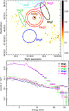 |
Fig. B.1. Exploration of the background and its impact in the high-energy spectrum of Apep. Top:NuSTAR image in the 20–35 keV energy range for FPMB (2022a). We indicate the position of Apep with a 30″ circle, the background extraction region used in the analysis (bkg1), and the alternative backgrounds used as independent checks (bkg2–bkg5). We also show with cyan contours the emission from the supernova remnant G330.2+1.0 obtained in the 2.5–8 keV range with XMM-Newton. The image is in linear scale (instead of logarithmic scale, as in Fig. 3), and it was smoothed in ds9 using a Gaussian with Radius=5. Bottom: Background-subtracted spectra (crosses) and background spectra (open circles) of Apep for the different background regions considered in Appendix B. In all cases, the whole data-set was co-added and rebinned to increase the S/N and to facilitate the visual comparison. |
We emphasise that the alternative backgrounds bkg2–bkg4 analysed here do not lie (at least not completely) within the same chip as the source, and they should therefore be taken with caution. Nonetheless, from this experiment, we conclude that a power-law component is statistically supported for all background regions considered. We highlight that the significance of the detection is lowest for bkg3 (≈1.66σ), and for the remaining regions, the significance is > 2σ. In particular, the significance of the detection for backgrounds within the same chip as the source (bkg1 and bkg5) is > 3.8σ. Finally, the flux of the power-law component fluctuates between F10 − 30 keV ∼ (1.3–4.8)×10−13 erg s−1 cm−2, depending on the background.
Complementarily, we followed a different approach to deal with uncertainties in the background. In this case, a background model was introduced and fitted using nuskybgd6 (Wik et al. 2014). The advantage of this approach is that the underlying background spectral model is well known, which limits the uncertainties to statistical ones. The total spectrum for the source region was extracted and then fitted with a fixed background model for that location. This was repeated for each observation and camera separately, using the five background regions discussed previously to have a good sampling of the background. The result is shown in Fig. B.2. In this case, a power-law component is again favoured, with a C-stat that diminishes from 682.4/589 to 666.3/588 when a power-law component is introduced. Similarly as discussed in Sect. 3, the overall decrease in C-stat is due to the better fit of the NuSTAR data, as the C-stat for the XMM-Newton cameras even increases slightly. This power-law component has a flux of  erg s−1 cm−2. The 90% confidence interval for the flux is F10 − 30 keV = (2.3–5.6)×10−13 erg s−1 cm−2, probing consistent results with those derived from fitting the background-subtracted spectra.
 |
Fig. B.2. NuSTAR spectra from the region of Apep for the two observations and cameras. This is not background subtracted, but instead, a background model was fitted using nuskybgd; the multiple components of this background model are shown as thin lines. The source model is TBabs*vphabs*(vpshock+po). |
Appendix C: Non-thermal emission model
We present a review of the multi-zone model we used to calculate the non-thermal radiation from Apep. This model is suitable for this CWB as the stars are separated by some tens of AU, which means that the shocks in the WCR are essentially adiabatic and quasi-stationary (del Palacio et al. 2022). The WCR structure is treated as an axisymmetric surface under a thin-shock approximation (i.e. the fluid is considered homogeneous along the direction perpendicular to the shock normal). The thermodynamical properties along the WCR (density, magnetic field intensity, etc.) are calculated with semi-analytical prescriptions based on mass and energy conservation of the fluid elements (Martinez et al. 2022), which is slightly more precise than the original assumption of Rankine-Hugoniot jump conditions in del Palacio et al. (2016). The only free parameter in the hydrodynamical model is the ratio of the thermal pressure (set by the properties of the stellar wind) and the magnetic pressure in the WCR, ηB.
Relativistic particles accelerate when a fluid line from a stellar wind enters the WCR. The relativistic particle distribution injected at a given position in the WCR is a power law with the spectral index given by the radio observations (p = 2.4). This distribution is normalised such that the injected power is a fraction fNT of the total power available for particle acceleration (Linj, ⊥). This power is distributed in electrons and protons as fNT = fNT, e + fNT, p. One common parametrisation is fNT, e = Ke, pfNT, with Ke, p ∼ 0.01 − 0.1 (see Merten et al. 2017, for a discussion of the uncertainties on this value). Upon injection, particles are attached to the fluid lines via the magnetic fields and flow together with the shocked fluid. As they stream, particles cool down due to different processes. The approximate solution used for the transport equation is given in Appendix A of del Palacio et al. (2022).
Finally, the non-thermal particles produce broadband radiation. The most relevant emission mechanisms are synchrotron and IC for electrons, which dominate in the radio and high-energy domain (hard X-rays and γ rays), and proton-proton collision for protons, which can contribute to the γ-ray flux (although this hadronic contribution is subdominant if Kep > 0.01). This emission is then corrected for absorption, namely free-free absorption in the ionised stellar winds for low-frequency radio emission, and γ-γ absorption in the stellar radiation fields for high-energy γ rays.
All Tables
Results of the fitting of NuSTAR and XMM-Newton spectra of Apep using different models.
All Figures
|
Fig. 1. RGB XMM-Newton image of the field of view of Apep (red = 0.3–1.2 keV, green = 1.2–2.5 keV, blue = 2.5–8 keV) from the EPIC-PN detector. We also indicate the position of the supernova remnant G330.2+1.0. |
| In the text | |
|
Fig. 2. Apep XMM-Newton spectra in the 0.3–10 keV energy range. In the left panel, the fitted model is TBabs*apec, and in the right panel, it is TBabs*vphabs*vpshock. The latter model is preferred as it leads to lower residuals between 1 and 2.5 keV. |
| In the text | |
|
Fig. 3. NuSTAR image in the 3–20 keV energy range for the 2022a (left panels) and 2022b observations (right panels). For each epoch and camera, we show the selected source and background extraction regions. Straylight can be seen at the bottom right corner of the FPMB observations. |
| In the text | |
|
Fig. 4. Apep NuSTAR spectra in the 3–35 keV energy range from co-adding the observations for each camera separately. In the left panel, the fitted model is TBabs*vphabs*vpshock, and in the right panel, an additional power-law component is added as TBabs*vphabs*(vpshock+po). |
| In the text | |
|
Fig. 5. Apep unfolded X-ray spectra in the 1–35 keV energy range with XMM-Newton and NuSTAR. The fitted models are constant*TBabs*vphabs*vpshock (left panel) and constant*TBabs*vphabs*(vpshock+po) (right panel). The spectra was rebinned for clarity. The fitted parameters are given in Table 3. |
| In the text | |
|
Fig. 6. Modelled broadband non-thermal SED of Apep. We show SEDs for the two extreme combinations of parameters that are compatible with the hard X-ray emission component detected with NuSTAR (this work) and with the ATCA radio data (Callingham et al. 2019). Dashed lines show the synchrotron component, dot-dashed lines show the IC component, dotted lines show the p-p component, and solid lines show the total SED. We also show the Fermi-LAT upper limits from Martí-Devesa et al. (2023) and the sensitivity curve for CTA (Funk et al. 2013). |
| In the text | |
|
Fig. A.1. Apep NuSTAR spectra in the 3–35 keV energy range. The spectra were further rebinned in XSPEC for clarity. The source spectrum is shown with crosses and the background spectrum with open circles. Top panel: Spectra for the 2022a and 2022b observations showing each camera separately. Middle panel: Spectrum from the co-added observations from both epochs (for each camera separately). Bottom panel: Spectrum from the co-added observations (both epochs, both cameras). |
| In the text | |
|
Fig. B.1. Exploration of the background and its impact in the high-energy spectrum of Apep. Top:NuSTAR image in the 20–35 keV energy range for FPMB (2022a). We indicate the position of Apep with a 30″ circle, the background extraction region used in the analysis (bkg1), and the alternative backgrounds used as independent checks (bkg2–bkg5). We also show with cyan contours the emission from the supernova remnant G330.2+1.0 obtained in the 2.5–8 keV range with XMM-Newton. The image is in linear scale (instead of logarithmic scale, as in Fig. 3), and it was smoothed in ds9 using a Gaussian with Radius=5. Bottom: Background-subtracted spectra (crosses) and background spectra (open circles) of Apep for the different background regions considered in Appendix B. In all cases, the whole data-set was co-added and rebinned to increase the S/N and to facilitate the visual comparison. |
| In the text | |
|
Fig. B.2. NuSTAR spectra from the region of Apep for the two observations and cameras. This is not background subtracted, but instead, a background model was fitted using nuskybgd; the multiple components of this background model are shown as thin lines. The source model is TBabs*vphabs*(vpshock+po). |
| In the text | |
Current usage metrics show cumulative count of Article Views (full-text article views including HTML views, PDF and ePub downloads, according to the available data) and Abstracts Views on Vision4Press platform.
Data correspond to usage on the plateform after 2015. The current usage metrics is available 48-96 hours after online publication and is updated daily on week days.
Initial download of the metrics may take a while.