| Issue |
A&A
Volume 693, January 2025
|
|
|---|---|---|
| Article Number | A266 | |
| Number of page(s) | 11 | |
| Section | Astrophysical processes | |
| DOI | https://doi.org/10.1051/0004-6361/202452599 | |
| Published online | 27 January 2025 | |
Chandra high-resolution spectra of Apep Plume: Exploring the colliding-wind picture in X-rays
Institute of Astronomy and National Astronomical Observatory (Bulgarian Academy of Sciences), 72 Tsarigradsko Chaussee Blvd., Sofia 1784, Bulgaria
⋆ Corresponding authors; szhekov@astro.bas.bg; bpetrov@astro.bas.bg
Received:
14
October
2024
Accepted:
2
December
2024
We present results of the first high-resolution observations of the massive Wolf-Rayet (WR) binary Apep Plume, taken with the Chandra High-Energy Transmission Grating in 2023 May. Analysis of these high-quality spectra showed that the spectral lines in this massive binary are broadened (full width at half-maximum, FWHM ≥ 2400 km s−1) and marginally blueshifted (∼ − 150 km s−1). A direct modelling of these spectra in the framework of the standard colliding stellar wind (CSW) picture provided a very good correspondence between the shape of the theoretical and observed spectra, but required a mass-loss reduction of 0.42 to be adopted. For a global view on this WR+WR binary, we performed a direct fitting of its optical spectrum by making use of stellar atmosphere models. The corresponding stellar parameters (mass-loss rate and wind velocities) from this analysis were used as input parameters for the CSW modelling of the X-ray emission from Apep Plume.
Key words: shock waves / stars: individual: Apep Plume / stars: winds / outflows / stars: Wolf-Rayet / X-rays: stars
© The Authors 2025
 Open Access article, published by EDP Sciences, under the terms of the Creative Commons Attribution License (https://creativecommons.org/licenses/by/4.0), which permits unrestricted use, distribution, and reproduction in any medium, provided the original work is properly cited.
This article is published in open access under the Subscribe to Open model. Subscribe to A&A to support open access publication.
1. Introduction
Wolf-Rayet (WR) stars are massive stars that have powerful winds and are losing mass at high rates (Ṁ ∼ 10−5 M⊙ yr−1; Vwind = 1000−5000 km s−1). Based on their optical spectra, they are divided into three subtypes: nitrogen-rich (WN), carbon-rich (WC), and oxygen-rich (WO). Their progenitors are massive stars with initial masses > 25 M⊙, and most WR stars are thought to end their lives as supernovae (see Crowther 2007 for a review on the physical properties of WRs).
If both components of a binary system are WR (or O) stars, the interaction of their massive stellar winds gives rise to a phenomenon known as colliding-stellar winds (CSWs): such a binary is referred to as a colliding-wind binary (CWB). The interaction region is bounded by two shocks, each compressing the stellar wind of the corresponding stellar component, and a contact discontinuity surface separating their shock plasmas.
Since the wind velocities are highly supersonic, the resultant post-shock temperatures are in the keV range; therefore, most of the plasma emission is in X-rays (e.g. Prilutskii & Usov 1976; Cherepashchuk 1976; see also Rauw & Nazé 2016 for a review on the progress of studies of X-ray emission from CWB). On the other hand, it is generally believed that CSWs are responsible for the non-thermal radio emission (or high-energy phenomena) in massive binaries (e.g. De Becker & Raucq 2013 and references therein) and for the periodic dust formation in WC binaries, as demonstrated by the prototype of the CSW binaries WR 140 (e.g. Williams et al. 1990).
Apep Plume (2XMM J160050.7−514245; WR 70−16) was serendipitously discovered as a bright X-ray source in the vicinity of the supernova remnant G330.2+01.0. Infrared observations revealed a dust plume with a size of ∼12 arcsec. It is a spatially resolved non-thermal radio source with a characteristic size of ∼47 mas. Optical observations resolved the binary components with an estimated binary separation of ∼47 mas. Based on optical spectroscopy, the binary components were classified as a WC8 and a WN4-6 object with wind velocity of 2100 km s−1 and 3500 km s−1, respectively. The optical observations also revealed that there is a star (likely an OB supergiant) within ∼0.7 arcsec of the WR binary. The X-ray emission of the Apep Plume originates from hot plasma with a typical temperature of ∼5 keV (for details of the observational findings, see Callingham et al. 2019, 2020; Han et al. 2020; Marcote et al. 2021). All these properties make Apep Plume a legitimate member of the CWB family.
To explore the physical picture of CSWs in Apep Plume in some detail, we need to confront the observational data with the corresponding theoretical model predictions. For this reason, we planned new X-ray observations of Apep Plume with high spectral resolution that were expected to provide X-ray spectra with better quality than achieved in the earlier observations of this object: all these observations provided only non-dispersed X-ray spectra.
This work presents the results from the first direct modelling of the X-ray emission (high-resolution spectra) from Apep Plume in the framework of the CSW picture. Our paper is organized as follows. In Sect. 2 we describe the high spectral resolution X-ray observations of Apep Plume. In Sect. 3 we analyse the profiles of strong X-ray emission lines. In Sect. 4 we give details about the CSW modelling of the X-ray spectra of Apep Plume and the corresponding results. In Sect. 5 we discuss our results, and we present our conclusions in Sect. 6.
2. Observations and data reduction
Chandra observed Apep Plume on four occasions during 2023 May with a total effective exposure of 94.96 ks (PI: S. Zhekov): Chandra Obs IDs 25895 (May 13; 26.80 ks; Obs 1), 25896 (May 13; 28.97 ks; Obs 2), 25126 (May 30; 14.71 ks; Obs 3), and 27879 (May 30; 24.48 ks; Obs 4). The observations were carried out with the high-energy transmission gratings (HETG), which has two spectral arms: medium-energy grating (MEG) and high-energy grating (HEG). Following the Science Threads for Grating Spectroscopy in the Chandra Interactive Analysis of Observations (CIAO) 4.161 data analysis software, we extracted the first-order X-ray spectra and the zero-order X-ray light curves (LCs) of Apep Plume from these data sets; we initially re-processed the data adopting the CIAO CHANDRA_REPRO script. In this study, we focus on the first-order MEG and HEG spectra.
The X-ray images for each observation are shown in Fig. 1, which illustrate the accuracy of the Chandra pointing. We constructed the background-subtracted light curves and found no variability on timescales shorter than the effective exposure of each observation. Specifically, using time bins from 100 to 1600 s (scaling bin size by a factor of 2), the X-ray LCs were statistically consistent with a constant flux. Adopting χ2 fitting, the LCs were fitted with a constant and the goodness of fit for the total light curve was ≥0.84 for all the cases of different binning. For the time bins 100, 200, 400, 800, and 1600 s, the reduced χ2 = 0.926, 0.935, 0.826, 0.770, 0.794 with the respective corresponding degrees of freedom 935, 486, 245, 123, 64.
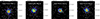 |
Fig. 1. Chandra images (0.5−10 keV) of Apep Plume (logarithmic intensity scale). RA (J2000) and Dec (J2000) are on the horizontal and vertical axes, respectively. The circled plus sign gives the near-infrared position of Apep Plume (SIMBAD). The asterisk gives the X-ray position derived by using the CIAO command WAVDETECT. |
Since no appreciable variability was detected, we constructed total HETG spectra of Apep Plume with a total number of source counts of 4212 (MEG) and 3054 (HEG). The Chandra calibration database CALDB v.4.11.0 was used to construct the response matrices and the ancillary response files. For the spectral analysis in this study, we made use of standard models and custom models in version 12.13.1 of XSPEC (Arnaud 1996).
3. Spectral lines
A general characteristic of the X-ray spectrum of Apep Plume in the 0.5−10 keV energy range is that the spectral lines are not very strong with respect to the underlying continuum. A physical reason for this could be that the X-ray emitting plasma is very hot. Thus, despite the acceptable quality of the HETG spectra, there are not many spectral lines that could be analysed in detail. We adopted various techniques (e.g. binning the spectra, using standard χ2-fitting, the Cash statistic; Cash 1979) and fits could provide line parameters only for the following lines: Fe XXV (1.85 Å), S XVI (4.73 Å), and Si XIV (6.18 Å).
We adopted the following model in the fits of the spectral lines. For the He-like triplet Fe XXV, the model was a sum of three Gaussians and a constant continuum. The centres of the triplet components were equal to their values given in the AtomDB data base (Atomic Data for Astrophysicists)2. All the components had the same line width and line shift. The free parameters of the fit were the common line shift, common line width, the individual fluxes of the three components, and the continuum level. For the H-like doublets S XVI and Si XIV, we used a similar model, but with a sum of two Gaussians and the component intensity ratios were fixed at their atomic data values.
To derive the line parameters, the MEG and HEG spectra were fitted simultaneously sharing all the same model parameters except for the continuum level. We worked with the unbinned spectra (with no background subtracted) and made use of the Cash statistic (Cash 1979) as implemented in XSPEC.
Figure 2 and Table 1 present the results from the fits to the spectral lines in the high-resolution spectra of Apep Plume. We note that the parameters of the Fe XXV He-like triplet are not constrained with the exception of the total observed line flux3. The strength of the intercombination and forbidden line components in the multiplet also seem to be in general agreement with their expected strength. This could be a sign that the Fe XXV complex forms in hot plasmas with relatively low density and located far from strong sources of UV emission. The latter could be considered a possible indication that these lines form in CSWs in wide massive binaries. However, we have to keep in mind that the quality of the X-ray spectrum near the Fe XXV line is not very good (only 35 cts in MEG and 109 cts in HEG), so future observations are needed to address this issue.
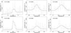 |
Fig. 2. Line profile fits to the He-like triplet of Fe XXV and the H-like doublets of S XVI and Si XIV in the first-order HETG spectra of Apep Plume. The spectra were rebinned for presentation purposes. |
Line parameters.
On the other hand, the H-like doublets of S XVI and Si XIV seem to be slightly blueshifted by ∼150 km s−1 and have line widths ≥2400 km s−1. Such line widths also seem to be consistent with the expectation that the X-ray spectrum of Apep Plume originates in CSWs. However, we again note the considerable uncertainties of these line parameters (see Table 1) that likely result from the photon statistics of S XVI (128 cts in MEG, 68 cts in HEG) and Si XIV (224 cts in MEG, 102 cts in HEG) lines.
4. CSW spectral modelling
We recall an important detail in the physical picture of Apep Plume, the presence of a third star (hereafter OB star), the likely OB supergiant at ∼0.7 arcsec from the central massive binary. We note that the X-ray emission from the OB star is soft (plasma temperatures considerably lower than 1 keV; e.g. Güdel & Nazé 2009), so we do not expect an appreciable contribution from this object to the total hard and luminous (high-luminosity) X-ray emission from Apep Plume. Therefore, we consider that the emission originates in CSWs in a massive WC+WN binary.
4.1. CSW model
In the framework of the standard CSW picture in massive binaries, we have two gas flows (stellar winds) colliding at their terminal velocities which results in a CSW interaction (shock) zone with a cylindrical symmetry. In turn, two-dimensional (2D) numerical hydrodynamic models could be used for calculating the physical parameters of this shock structure. Such a CSW structure should be considered typical for the case of wide binary systems (as Apep Plume; see Sect. 4.2), where radiative braking (Gayley et al. 1997) and radiative inhibition (Stevens & Pollock 1994) are not expected to play an important role. The same is valid for the orbital motion because orbital velocities are much slower than the wind velocities. A schematic diagram of the CSW region is shown in Fig. 3. We adopt the convention that the massive star with the weaker wind (that with the smaller ram pressure) is located at the origin of the coordinate system.
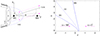 |
Fig. 3. Physical picture of CSWs in massive banaries. Left panel: Schematic presentation of the CSW region in massive WC+WN binary. The label CSW marks the wind interaction region, which is a 3D structure with its axis of symmetry Z. The axes X and Y complete the Cartesian coordinate system. The two angles i (orbital inclination) and α (azimuthal angle) define the orientation in space of the line of sight (l.o.s.) towards the observer. The label ‘Velocity’ denotes the general direction of the shocked plasma flow. The two dashed-line arrows illustrate that emission from a parcel of gas in the CSW region is subject to different wind absorption, depending on the orientation (i, α) of the l.o.s. towards the observer and the rotational angle around the axis of symmetry (Z). Right panel: CSW region derived from the 2D hydrodynamic simulations for the adopted values of the stellar-wind parameters in Apep Plume which give a wind-momentum rate ratio of the stellar winds of Λ = 4.86. The x- and z-axes are in units of the binary separation. The WC and WN components are located at (x, z) coordinates (0, 0) and (0, 1), respectively. The solid lines mark the shock fronts and the dashed line marks the contact discontinuity. The half opening angle of the WC shock (WC), contact discontinuity (CD), and the WN shock (WN) ‘cones’ is ∼47°, ∼64°, and ∼84°, respectively. |
As demonstrated by the first CSW hydrodynamic models for massive binaries (Lebedev & Myasnikov 1990; Luo et al. 1990; Stevens et al. 1992; Myasnikov & Zhekov 1993), the basic input parameters for the hydrodynamic simulations are the mass loss and velocity of the stellar winds of the binary components and the binary separation. We note that the shape and the structure of the CSW interaction region are defined by the wind-momentum rate ratio of the stellar winds of the binary components: a dimensionless parameter Λ = (ṀWNVWN)/(ṀWCVWC) (in the case of the WC+WN binary Apep Plume).
We recall that our XSPEC CSW model is based on the 2D numerical hydrodynamic model of adiabatic CSW by Lebedev & Myasnikov (1990) (see also Myasnikov & Zhekov 1993). It can take into account partial electron heating in strong shocks (see Zhekov & Skinner 2000), non-equilibrium ionization (NEI) effects (see Zhekov 2007), line broadening due to the bulk gas velocity of the emitting plasma (see Zhekov & Park 2010), the specific stellar wind absorption of both binary components along the line of sight to the observer (see Zhekov 2021), and the different chemical composition of both stellar winds. For a direct fitting of an observed X-ray spectrum with the CSW model in XSPEC, we must know the distance to the studied object. For a detailed description of the CSW model and the fitting procedure with the CSW model in XSPEC, we refer to Sect. 4.1 of Zhekov (2017) and Sect. 4.1 of Zhekov (2021).
4.2. CSW model parameters for Apep Plume
As mentioned above, the basic input parameters for the CSW hydrodynamic model and in XSPEC are the stellar wind parameters of the binary components (mass-loss rates, wind velocities), binary separation, and distance to the studied object. These parameters are usually derived from analysis of the optical spectra and the radio emission of massive stars.
From a standard analysis of optical spectra of Apep Plume, obtained with the X-SHOOTER spectrograph on the European Southern Observatory (ESO) Very Large Telescope (VLT), Callingham et al. (2020) measured the terminal wind velocities of both components of the WC+WN binary. On the other hand, the mass-loss rates were estimated from analysis of the non-thermal radio emission by addressing its corresponding free-free absorption in the stellar winds (del Palacio et al. 2022).
To derive all these parameters in a more consistent way, we modelled the above-mentioned high-resolution optical spectra of Apep Plume using stellar-atmosphere models. We adopted a novel technique to fit the composite (total) spectrum of a massive binary: a 4D grid modelling of UV-optical spectra. Details of this fitting procedure and the corresponding results are given in Appendix A. Here we provide the derived parameter values used in the CSW model: ṀWC = 1.29 × 10⁻⁵ and ṀWN = 4.47 × 10⁻⁵ (M⊙ yr−1); VWC = 2374 and VWN = 3332 (km s−1).
From an analysis of near-infrared data, Han et al. (2020) constrained the projected binary separation of 47 ± 5 mas. This study and that by del Palacio et al. (2022) suggested that we observe the central binary in Apep Plume almost pole on, that is along the X-axis in Fig. 3. Since the distance to this object is not well constrained, in this study we adopt a distance of 2.4 kpc (Callingham et al. 2019). Therefore, the separation between the stellar components in the WC+WN binary in Apep Plume is 112.7 au.
For this set of stellar and binary parameters, we see that the CSW shocks in Apep Plume are adiabatic. Specifically, using Eq. (8) from Stevens et al. (1992), the cooling parameter introduced therein has values χ > 130 for both stellar winds (shocks are adiabatic if χ > 1). Using Eq. (9) from Myasnikov & Zhekov (1993), the cooling parameter has values Γff < 3.3 × 10⁻⁴ for both stellar winds (shocks are adiabatic if Γff ≪ 1). In addition, the shock-heated plasma may have different electron and ion temperatures (Te ≠ Ti; using Eq. (1) from Zhekov & Skinner 2000), and the NEI effects may play some role (using Eq. (1) from Zhekov 2007).
4.3. CSW model spectral results
We note that the orbital parameters of Apep Plume are not well constrained: we have an estimation of the binary separation and we likely observe the WC+WN binary pole on. Thus, we considered modelling the CSW X-ray emission for an inclination angle of i = 0 deg (Fig. 3). It is worth noting that in such a case the CSW spectra do not depend on the azimuthal angle, meaning that they are the same for each value of α ∈ [0, 180] deg. Due to the symmetry of the CSW region, the CSW models with a given value of α and 360 − α give identical spectra.
In addition, we explored a range of values for the partial heating of the electrons at the shock fronts. The adopted set was β = [0.001, 0.01, 0.05, 0.1, 0.2, 0.3, 0.4, 0.5, 0.6, 0.7, 0.8, 0.9, 1]; β = Te/T, Te is the electron temperature, and T is the mean plasma temperature (β < 1 → 2 − T plasma, different electron and ion temperatures; β = 1 → 1 − T plasma, equal ion and electron temperatures).
In general, there are two components of the X-ray absorption: (a) due to the interstellar matter (ISM); (b) due to the stellar wind(s) in Apep Plume. Anticipating the spectral fit results, we note that we did not find any improvement of the spectral fits if we took into account the wind absorption (component b). This is likely due to the fact that WR is a very wide binary system observed pole-on; the wind absorption could have had some impact on the CSW spectrum if the inclination angle were large (e.g. close to 90 deg).
For a consistent global physical picture of Apep Plume, we fixed the X-ray absorption (the ISM component) to have column density NH = 2.18 × 1022 cm−2. For this, we used the derived value of the ISM reddening of the optical spectrum of Apep Plume (Appendix A) and the conversion NH = 1.65 (1.6 − 1.7)×1021AV cm−2 (Vuong et al. 2003; Getman et al. 2005).
In the framework of this global physical picture, the chemical composition of the shocked WC and WN winds have the same abundances as in our analysis of the optical spectrum of Apep Plume (Appendix A). We adopted the abundance values typical for the WC and WN stars (by number) from van der Hucht et al. (1986). Ar and Ca are not present in the van der Hucht et al. (1986) abundance sets, so we adopted for each of them a fiducial value of 2 × 10⁻⁵. For the WC shocked wind we adopted H = 0.0, He = 1.0, C = 0.4, N = 0.0, O = 0.194, Ne = 1.86 × 10⁻², Mg = 2.72 × 10⁻³, Si = 6.84 × 10⁻⁴, S = 1.52 × 10⁻⁴, Ar = 2 × 10⁻⁵, Ca = 2 × 10⁻⁵, and Fe = 3.82 × 10⁻⁴. For the WN shocked wind we adopted H = 0.067, He = 1.0, C = 1.28 × 10⁻⁴, N = .29 × 10−3, O = 2.92 × 10⁻⁴, Ne = 6.57 × 10⁻⁴, Mg = 2.19 × 10⁻⁴, Si = 2.16 × 10⁻⁴, S = 5.11 × 10⁻⁵, Ar = 2 × 10⁻⁵, Ca = 2 × 10⁻⁵, and Fe = 1.28 × 10⁻⁴.
In all the spectral fits, the NEI effects were taken into account. To improve the quality of the fits, we allowed some abundances to vary (e.g. Mg, Si, S, and Fe). Because the X-ray emission from the shocked WC and WN winds cannot be disentangled, the abundance of a given element was varied by a single scaling parameter for both parts of the CSW region with respect to their reference abundances. Our results are from simultaneous fits to the MEG and HEG spectra of Apep Plume in the 0.5−10 keV energy range (1.24−24.8 Å). The spectra were rebinned to have a minimum of 20 counts per bin to improve the photon statistics (i.e. for a better constraint of the derived parameters).
CSW spectral fit results.
For the 13 cases under consideration (β ∈ [0.001, 1]), the fits had acceptable quality (reduced χ2 < 1); this means that the shape of the observed spectra is matched very well, and the basic result is that NORM parameter of our CSW model in XSPEC had values in the range [0.171, 0.184]. We recall (see Sect. 4.1 in Zhekov 2017 and Sect. 4.1 in Zhekov 2021) that we are dealing with X-ray emission from thermal plasma and NORM = 1 (resp. NORM < 1, NORM > 1) shows whether the theoretical model predicts an amount of emission measure exactly as needed (resp. higher, lower than that) to explain the observed X-ray emission. Since the emission measure of collisionally excited hot plasma is proportional to the square of its number density (number density in the CSW region is proportional to the mass-loss rate); therefore, a mass-loss rate reduction (Ṁs) in the range [0.41, 0.43] is needed to have NORM ≈ 1.
As our fitting procedure requires, we repeated its steps: we re-ran the hydrodynamic model; we prepared the input parameters for the spectral model anew (e.g. distribution of temperature, emission measure, ionization age); and we fitted the HETG spectra in XSPEC. The quality of the CSW spectral fits is shown in Fig. 4. The results for formally the best fit (β = 0.6) are given in Fig. 5 and Table 2.
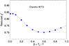 |
Fig. 4. Reduced χ2 values (degrees of freedom, d.o.f. = 343) as a function of partial heating at the shock fronts (β = Te/T) for the case of reduced mass-loss rates. The magenta circle marks the formal minimum value of the reduced χ2 at β = 0.6. |
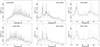 |
Fig. 5. The background-subtracted HETG (MEG – first row; HEG – second row) spectra of Apep Plume, overlaid with the best-fit model spectrum with β = 0.6. The spectra were rebinned to have a minimum of 20 counts per bin. |
We see that the theoretical CSW model spectrum matches very closely the observed high-resolution X-ray spectra of Apep Plume. The line profile of the best spectral line (i.e. with the best photon statistics) in the spectrum (Si XIV 6.18 Å) seems to be closely matched as well (see Col. 3 in Fig. 5). However, this does not seem to be the case for the line profile of the Si XIII line (6.65 Å), which is quite weak (i.e., its photon statistics are not very good). It is worth noting that it is hard to draw a general conclusion about the theory versus observations issue for the spectral line profiles because there are just two spectral lines in Apep Plume that could be analysed, as mentioned earlier in Sect. 3.
We note that for the adopted distance of 2.4 kpc the X-ray luminosity of Apep Plume in relatively soft X-rays (0.5−10 keV spectral range) makes it the second or even third most X-ray luminous WR star in the Galaxy after the WC+WN binary WR 48a (e.g. Zhekov et al. 2022 and references therein). The X-ray luminosity of Apep Plume is about equal to the mean luminosity over the orbital period of the prototype CSW binary WR 140 (see Fig. 10 in Zhekov 2021). We consider only WR binaries without a degenerate object, so we excluded the black hole candidate Cyg X-3, which is an ultra-luminous X-ray source, with X-ray luminosity > 5.5 × 1038 ergs s−1 (Veledina et al. 2024).
In general, it seems reasonable to conclude that the observed characteristics of the WC+WN binary in Apep Plume could be explained in a coherent physical picture; analysis of its optical emission provides the corresponding physical characteristics of the massive stars in the binary. These characteristics determine the properties of the resultant CSW region in the binary, whose purely thermal emission closely matches the observed X-ray emission from this system in the 0.5−10 keV energy range. This means that the contribution from non-thermal X-rays reported at high energies (10−30 keV) by del Palacio et al. (2023) is negligible in soft X-rays (0.5−10 keV)4. The same is valid for the X-ray emission from the WC and WN components themselves. We recall that single WC stars are likely very faint or X-ray quiet objects (Oskinova et al. 2003; Skinner et al. 2006; Anastasopoulou et al. 2024). In contrast, single WN stars are X-ray sources with luminosities < 1033 ergs s−1 (Skinner et al. 2010, 2012). However, there are details in the CSW physical picture in Apep Plume that need additional discussion.
5. Discussion
We analysed the first high-resolution X-ray spectra of Apep Plume that includes a direct modelling of the observed spectra in the framework of the standard colliding stellar wind picture in a massive WC+WN binary. Two of the basic results from this analysis are the following.
First, the emission lines in the X-ray spectrum of Apep Plume are not very strong, so only three of them (Fe XXV 1.85 Å, S XVI 4.73 Å, Si XIV 6.18 Å) could be subject to a standard line-profile analysis. Although the uncertainties of the derived parameters are not small (see Table 1), the results are within the expectations from the CSW picture. Namely, lines that form in cooler plasma are broader than those originating in hotter plasma. We recall that the CSW region is temperature-stratified and the hotter plasmas are near the axis of symmetry of the interaction region (axis Z in Fig. 3). Since the shocks are oblique, the bulk velocity of the cooler plasmas is higher than that of the hotter plasmas. The small (consistent with zero) line blueshifts are also expected if we observe the massive binary at very low inclination (e.g. almost along axis X in Fig. 3).
Second, the direct fitting of the observed X-ray spectra with the CSW model showed a very good correspondence between theory and observations, provided we adopt a scaling factor of Ṁs = 0.42 to the mass-loss rates in the binary. We note that the stellar wind parameters for the CSW model were derived from our analysis of the optical spectrum of Apep Plume by making use of stellar atmosphere models (see Appendix A). We recall that in the framework of stellar atmosphere models, mass-loss rate and luminosity depend on the distance to the studied object: Ṁ ∝ d1.5, L⋆ ∝ d2 (see Eqs. (1) and (4) from Hillier & Miller 1999; also Schmutz et al. 1989). So, for a mass-loss reduction of Ṁs = 0.42, a corresponding distance value of 0.56× the value adopted in this study (2.4 kpc) might be a possible explanation. It is also worth noting that the distance to this object is still quite uncertain. There is no Gaia distance to Apep Plume; moreover, Apep Plume has no Gaia identifier (name) in SIMBAD. All this leaves some ‘wiggle room’ in some details with this parameter, but we do not see it as a reasonable way to go.
On the one hand, if we adopt a distance reduction of a factor of 0.56, it will result in a lower value (by 0.50 dex) for the luminosities (log L⋆ in units of L⊙) derived in our analysis of the optical spectrum of Apep Plume. These luminosities would be somewhat on the weak side for WR stars, more so for the WC component (see e.g. Table 1 in Sander et al. 2019 and in Hamann et al. 2019; see also Appendix A).
On the other hand, there is a scaling law in the CSW model that allows us to estimate the impact of distance change on the X-ray emission from the interaction region (Luo et al. 1990; Myasnikov & Zhekov 1993). Namely, the X-ray luminosity is a function of the mass-loss rate (Ṁ), wind velocity (v), and binary separation (D): LX ∝ Ṁ2v−3D−1. Since the wind velocity does not depend on the distance to the studied object, while for a spatially resolved binary such as Apep Plume binary separation is proportional to distance (d), we have LX ∝ Ṁ2d−1. In turn, it follows that the CSW total flux (and flux density) is FX ∝ Ṁ2d−3. So, taking into account the above-mentioned mass-loss dependence on distance (Ṁ ∝ d1.5), we see that the properties of the CSW spectrum for spatially resolved binaries are invariant with the distance to the studied object. In other words, if we have derived the characteristics of the stellar components in a spatially resolved massive binary for a specific value of the distance, playing with the distance value does not change the properties of the X-ray emission from the CSW region in this system, but it will change its X-ray luminosity. Therefore, it is not possible to resolve the mass-loss reduction issue for Apep Plume by simply choosing a different distance value to this object.
We note that there is a way to adopt a mass-loss scaling in the framework of the stellar atmosphere models for the optical emission from massive stars. Because their spectra result mostly from two-particle collisions and their winds are clumpy, it is generally assumed that the spectrum of a massive star, with other stellar parameters kept fixed, will be practically the same for mass-loss rates that scale with their corresponding volume filling factors (f∞):  (for numerical tests on this issue see Sect. 4.3 in Petrov & Zhekov 2024). Since the stellar parameters of the massive stars in Apep Plume are derived adopting a value of f∞ = 0.1 (Appendix A), the mass-loss rate reduction of Ṁs = 0.42 will suggest that the volume filling factor of the stellar winds should be rather small: f∞ = 0.01764.
All this underlines what was already brought up from the CSW modelling of X-ray emission in wide WR binaries WR 147, WR 140, WR 48a (Zhekov et al. 2020, 2022; Zhekov 2021). Specifically, if the clumps occupy such a small part of the stellar wind (f∞ ≤ 0.1), we need to know how clumps manage to collide and form the CSW region.
As a possible solution, we reiterate an earlier suggestion (see Sect. 4.3 in Zhekov et al. 2020) that the stellar winds of massive stars are two-component flows: dense clumps with (even small) filling factor f∞ and a low-density component occupying 1 − f∞ of the volume. The low-density components of the stellar winds in the binary easily collide and form a basic CSW region. Then, the dense clumps are dissolved in the CSW region and provide the strong X-ray emission observed from massive binaries. If the dense clumps are not dissolved very efficiently (e.g. some clumps may pass through the basic CSW region like bullets), then in X-rays we will not observe part of the stellar wind mass that has been detected in the optical. This means that there might be some trade-off between the amount of clumping in the stellar winds and the efficiency of the mechanism providing the way the dense clumps dissolve in the CSW region.
It is worth recalling here that based on 2D numerical hydrodynamic simulations of clumpy CSWs in wide binaries, Pittard (2007) concluded that clumps are quickly heated up and dissolved in it after crossing the shock fronts of the CSW region. However, these simulations considered only one specific case of the volume filling factor for the clumps (and other physical parameters of the wide stellar binary). Thus, a parameter study of the clump-CSW-region interaction is needed. Such a study will also explicitly require 3D hydrodynamic simulations.
6. Conclusions
The basic results and conclusions from our analysis of the first high spectral resolution X-ray spectra (Chandra HETG) of Apep Plume in the framework of the CSW picture in massive binaries that incorporates the results from modelling the optical emission of this object are the following:
(i) A general characteristic of the X-ray spectrum of Apep Plume in the 0.5−10 keV energy range is that the spectral lines are not very strong with respect to the underlying continuum. Thus, line parameters were derived only for three spectral lines: Fe XXV (1.85 Å), S XVI (4.73 Å), Si XIV (6.18 Å). Despite the appreciable uncertainties, the S XVI and Si XIV lines seem to be slightly blueshifted by ∼150 km s−1 and have line widths ≥2400 km s−1, while these line parameters are not constrained for the Fe XXV line due to the quality of the data.
(ii) A direct modelling of these Chandra (MEG, HEG) spectra in the framework of the standard CSW picture provided a very good correspondence between the shape of the theoretical and observed spectra, but a mass-loss reduction of 0.42 is required for full consistency between theory and observations.
(iii) For the adopted distance of 2.4 kpc, the X-ray luminosity of Apep Plume in the 0.5–10 keV spectral range (log LX = 34.39 ergs s−1) makes it the third most X-ray luminous WR star in the Galaxy amongst the WR binaries without a degenerate companion: WR 48a; WR 140; Apep Plume.
(iv) For a coherent global view on this massive WC+WN binary, we performed a direct fitting of its optical spectrum by making use of stellar atmosphere models. Thus, the derived stellar parameters (mass-loss rate and wind velocity) were used as input parameters for the CSW modelling of the X-ray emission from Apep Plume.
Data availability
The X-ray data underlying this research are public and can be accessed as follows. The Chandra data sets can be downloaded from the Chandra X-ray observatory data archive https://cxc.harvard.edu/cda/ by typing in the target name (Apep Plume) in the general search form https://cda.harvard.edu/chaser/. The X-Shooter optical spectra can be downloaded from the ESO data archive by typing in the target name in the following search form http://archive.eso.org/wdb/wdb/adp/phase3_spectral/form
For CIAO, see https://cxc.harvard.edu/ciao/
For AtomDB, see http://www.atomdb.org/
The resolution element (FWHM) is 0.023 Å (MEG) and 0.012 Å (HEG) or correspondingly 3730 km s−1 and 1946 km s−1 (see Table 8.1 in the Chandra Proposers’ Observatory Guide; http://asc.harvard.edu/proposer/POG/html/index.html).
For the ESO Science Archive see http://archive.eso.org/cms.html
Acknowledgments
This research has made use of data and/or software provided by the High Energy Astrophysics Science Archive Research Center (HEASARC), which is a service of the Astrophysics Science Division at NASA/GSFC and the High Energy Astrophysics Division of the Smithsonian Astrophysical Observatory. This research has made use of the NASA’s Astrophysics Data System, and the SIMBAD astronomical data base, operated by CDS at Strasbourg, France. Based on data obtained from the ESO Science Archive Facility under request 586438. The authors thank an anonymous referee for valuable comments and suggestions.
References
- Anastasopoulou, K., Guarcello, M. G., Flaccomio, E., et al. 2024, A&A, 690, A25 [NASA ADS] [CrossRef] [EDP Sciences] [Google Scholar]
- Arnaud, K. A. 1996, in Astronomical Data Analysis Software and Systems, eds. G. H. Jacoby, & J. Barnes, ASP Conf. Ser., 101, 17 [NASA ADS] [Google Scholar]
- Asplund, M., Grevesse, N., Sauval, A. J., & Scott, P. 2009, ARA&A, 47, 481 [NASA ADS] [CrossRef] [Google Scholar]
- Callingham, J. R., Tuthill, P. G., Pope, B. J. S., et al. 2019, Nat. Astron., 3, 82 [Google Scholar]
- Callingham, J. R., Crowther, P. A., Williams, P. M., et al. 2020, MNRAS, 495, 3323 [NASA ADS] [CrossRef] [Google Scholar]
- Cash, W. 1979, ApJ, 228, 939 [Google Scholar]
- Cherepashchuk, A. M. 1976, Soviet. Astron. Lett., 2, 138 [NASA ADS] [Google Scholar]
- Crowther, P. A. 2007, ARA&A, 45, 177 [Google Scholar]
- De Becker, M., & Raucq, F. 2013, A&A, 558, A28 [NASA ADS] [CrossRef] [EDP Sciences] [Google Scholar]
- del Palacio, S., Benaglia, P., De Becker, M., Bosch-Ramon, V., & Romero, G. E. 2022, PASA, 39, e004 [NASA ADS] [CrossRef] [Google Scholar]
- del Palacio, S., García, F., De Becker, M., et al. 2023, A&A, 672, A109 [NASA ADS] [CrossRef] [EDP Sciences] [Google Scholar]
- Fitzpatrick, E. L. 1999, PASP, 111, 63 [Google Scholar]
- Gayley, K. G., Owocki, S. P., & Cranmer, S. R. 1997, ApJ, 475, 786 [Google Scholar]
- Getman, K. V., Feigelson, E. D., Grosso, N., et al. 2005, ApJS, 160, 353 [NASA ADS] [CrossRef] [Google Scholar]
- Güdel, M., & Nazé, Y. 2009, A&ARv, 17, 309 [Google Scholar]
- Hamann, W. R., Gräfener, G., Liermann, A., et al. 2019, A&A, 625, A57 [NASA ADS] [CrossRef] [EDP Sciences] [Google Scholar]
- Han, Y., Tuthill, P. G., Lau, R. M., et al. 2020, MNRAS, 498, 5604 [NASA ADS] [CrossRef] [Google Scholar]
- Hillier, D. J., & Lanz, T. 2001, in Spectroscopic Challenges of Photoionized Plasmas, eds. G. Ferland, & D. W. Savin, ASP Conf. Ser., 247, 343 [NASA ADS] [Google Scholar]
- Hillier, D. J., & Miller, D. L. 1998, ApJ, 496, 407 [NASA ADS] [CrossRef] [Google Scholar]
- Hillier, D. J., & Miller, D. L. 1999, ApJ, 519, 354 [Google Scholar]
- Lebedev, M. G., & Myasnikov, A. V. 1990, Fluid Dynamics, 25 [Google Scholar]
- Luo, D., McCray, R., & Mac Low, M.-M. 1990, ApJ, 362, 267 [CrossRef] [Google Scholar]
- Marcote, B., Callingham, J. R., De Becker, M., et al. 2021, MNRAS, 501, 2478 [NASA ADS] [CrossRef] [Google Scholar]
- Myasnikov, A. V., & Zhekov, S. A. 1993, MNRAS, 260, 221 [NASA ADS] [Google Scholar]
- Oskinova, L. M., Ignace, R., Hamann, W. R., Pollock, A. M. T., & Brown, J. C. 2003, A&A, 402, 755 [NASA ADS] [CrossRef] [EDP Sciences] [Google Scholar]
- Petrov, B. V., & Zhekov, S. A. 2024, ArXiv e-prints [arXiv:2410.04881] [Google Scholar]
- Pittard, J. M. 2007, ApJ, 660, L141 [NASA ADS] [CrossRef] [Google Scholar]
- Prilutskii, O. F., & Usov, V. V. 1976, Soviet Ast., 20, 2 [NASA ADS] [Google Scholar]
- Rauw, G., & Nazé, Y. 2016, Adv. Space Res., 58, 761 [Google Scholar]
- Sander, A. A. C., Hamann, W. R., Todt, H., et al. 2019, A&A, 621, A92 [NASA ADS] [CrossRef] [EDP Sciences] [Google Scholar]
- Schmutz, W., Hamann, W. R., & Wessolowski, U. 1989, A&A, 210, 236 [Google Scholar]
- Skinner, S., Güdel, M., Schmutz, W., & Zhekov, S. 2006, Ap&SS, 304, 97 [NASA ADS] [CrossRef] [Google Scholar]
- Skinner, S. L., Zhekov, S. A., Güdel, M., Schmutz, W., & Sokal, K. R. 2010, AJ, 139, 825 [Google Scholar]
- Skinner, S. L., Zhekov, S. A., Güdel, M., Schmutz, W., & Sokal, K. R. 2012, AJ, 143, 116 [Google Scholar]
- Stevens, I. R., & Pollock, A. M. T. 1994, MNRAS, 269, 226 [Google Scholar]
- Stevens, I. R., Blondin, J. M., & Pollock, A. M. T. 1992, ApJ, 386, 265 [Google Scholar]
- van der Hucht, K. A., Cassinelli, J. P., & Williams, P. M. 1986, A&A, 168, 111 [NASA ADS] [Google Scholar]
- Veledina, A., Muleri, F., Poutanen, J., et al. 2024, Nat. Astron., 8, 1031 [NASA ADS] [CrossRef] [Google Scholar]
- Vuong, M. H., Montmerle, T., Grosso, N., et al. 2003, A&A, 408, 581 [NASA ADS] [CrossRef] [EDP Sciences] [Google Scholar]
- Williams, P. M., van der Hucht, K. A., Pollock, A. M. T., et al. 1990, MNRAS, 243, 662 [NASA ADS] [Google Scholar]
- Zhekov, S. A. 2007, MNRAS, 382, 886 [Google Scholar]
- Zhekov, S. A. 2017, MNRAS, 472, 4374 [NASA ADS] [CrossRef] [Google Scholar]
- Zhekov, S. A. 2021, MNRAS, 500, 4837 [Google Scholar]
- Zhekov, S. A., & Park, S. 2010, ApJ, 721, 518 [NASA ADS] [CrossRef] [Google Scholar]
- Zhekov, S. A., & Skinner, S. L. 2000, ApJ, 538, 808 [Google Scholar]
- Zhekov, S. A., Petrov, B. V., Tomov, T. V., & Pessev, P. 2020, MNRAS, 494, 4525 [CrossRef] [Google Scholar]
- Zhekov, S. A., Gagné, M., & Skinner, S. L. 2022, MNRAS, 510, 1278 [Google Scholar]
Appendix A: 4D grid-fitting of the optical spectrum of Apep Plume
Our task here was to derive the basic stellar parameters (effective temperature, luminosity, mass-loss rate, wind velocity; (T*, L⋆, Ṁ and v∞) of the massive stars in Apep Plume from a direct modelling (fitting) of the high-resolution optical spectrum of this object. For this goal, we made use of our recent technique we refer to as 4D grid-fitting because it is based on model atmosphere spectra with specific values for the basic four stellar parameters. Details about this technique (e.g. methods, numerical uncertainties) are found in Petrov & Zhekov (2024).
A.1. Optical spectrum of Apep Plume
Optical spectra of Apep Plume were taken from the public archive of the European Southern Observatory (ESO).5 The corresponding observations [Program ID: 0103.D-0695(A)] were carried out with the X-SHOOTER spectrograph at the ESO’s Very Large Telescope (VLT) in 2019 May. Details about the observations and the standard spectral analysis are found in Callingham et al. (2020). We note that the archive spectra are wavelength and flux calibrated (ESO Phase 3 Data Release).
We used the science spectrum from all the nine individual exposures to create the mean optical spectrum of Apep Plume in the spectral range of 5000 - 11000 Å. The quality of the spectra below 5000 Å is very poor and unfortunately the spectra are not useful at those wavelengths. For our analysis, we considered two cases of 1Å and 2Å sampling of the mean spectrum. The errors of the mean spectrum (at each spectral bin) are the standard deviation for the set of the nine individual exposures, because the scatter between individual spectra is the dominant source for the mean spectrum noise.
We recall that apart from the central WC+WN binary in Apep Plume, there is an OB star at ∼0.7 arcsec from the central binary (Callingham et al. 2019, 2020). Given the X-SHOOTER set-up, the observed spectrum of Apep Plume is actually a composite spectrum; namely, it is a sum of a WC, WN, and OB star spectrum. For the central massive binary is a very wide binary we observe at very low inclination, we do not expect any wind-absorption effects for either of the WR spectra by the wind of its binary companion. The same is valid for the OB star spectrum, because this object is at a distance much larger than the binary separation of the central binary. So, we consider that the observed optical spectrum of Apep Plume is a sum of three spectra (WC, WN and O) subject to common reddening (interstellar absorption). The latter is a reasonable assumption we believe: if the OB star were located closer to us, thus, being less reddened, we would have detected its spectrum at wavelengths shorter than 5000 Å but this is not the case in the X-SHOOTER observations.
Therefore, for the 4D grid-fitting of the optical spectrum of Apep Plume, we need a theoretical spectrum that is a sum of a WC, WN, and OB star spectrum. This means that three different 4D grids of model spectra are needed for this task.
A.2. 4D grids of model spectra and fitting procedure
Details about the procedure for creating 4D grids of model spectra for massive stars are given in Petrov & Zhekov (2024) and here we outline some basics of theirs. The grids are built using the non-local thermal equilibrium (non-LTE) radiative transfer code CMFGEN (Hillier & Miller 1998; Hillier & Lanz 2001)6, adopting constant volume filling factor f∞ = 0.1. Here, we used the same WC grid described in Petrov & Zhekov (2024) and the WN grid and the O grid are new ones dedicated for the goal of this study.
WC grid. The parameter ranges are: log Ṁ = [-5.0, -4.8, -4.5, -4.3] in M⊙ yr−1, log L⋆ = [4.8, 5.2, 5.4, 5.6, 5.8] L⋆ in L⊙, T* = [45 000, 50 000, 55 000, 60 000, 65 000, 70 000, 80 000, 90 000, 100 000, 110 000, 120 000] K and v∞ = [1 500, 2 000, 3 000] km s−1, resulting in a total number of 792 model spectra. The adopted WC abundances are from van der Hucht et al. (1986).
WN grid. The parameter ranges are: log Ṁ = [-4.5, -4.3] in M⊙ yr−1, log L⋆ = [5.2, 5.4, 5.6] L⋆ in L⊙, T* = [60 000, 65 000, 70 000, 80 000, 90 000, 100 000] K and v∞ = [2 250, 3 400] km s−1, resulting in a total number of 72 model spectra. The adopted WN abundances are from van der Hucht et al. (1986).
OB star grid. The parameter ranges are: log Ṁ = [-6.0, -5.75] in M⊙ yr−1, log L⋆ = [4.5, 4.75, 5.0] L⋆ in L⊙, T* = [12 500, 15 000, 17 500] K and v∞ = [500, 1 000] km s−1, resulting in a total number of 36 model spectra. The adopted abundances are from Asplund et al. (2009).
A new feature here (a procedure upgrade) is that the theoretical model spectrum is a sum of three different spectra: WC+WN+O spectrum. It is important to note that these spectra are indeed independent vectors, because none of them could mimic any of the other two spectra. Thus, at each step of the fitting process a spectrum is calculated from each of the grids and the sum of the three components defines the total spectrum.
Since we fit an observed spectrum in absolute units, our 4D grid-fitting procedure requires a distance value to the studied object. A distance of 2.4 kpc to Apep Plume is adopted (Callingham et al. 2019). In all the fits, we used the Galactic extinction curve of Fitzpatrick (1999) with RV = 3.1.
4D grid-fitting results for Apep Plume
A.3. 4D grid-fitting results
As described in Petrov & Zhekov (2024), our 4D fitting procedure is based on searching the minimum of four similarity functions (robust likelihood estimators). In the case of Apep Plume, these fits were done for the cases of the optical spectrum with actual errors and with no errors. We repeated them for the two cases of sampling of the optical spectrum with 1Å and 2Å, respectively, to explore the effects of spectral resolution. Thus, we have 16 sets of fit results and they define the numerical accuracy of our procedure. The corresponding results are given in Table A.1 and Fig. A.1 the quoted uncertainties are the standard deviations of the 16 values for each parameter. The relatively small value for the standard deviations are sign that all the fits converge very closely. This gives us confidence in the results from our 4D grid-fitting to the optical spectrum of Apep Plume.
For consistency with the CSW modelling of the X-ray emission from Apep Plume (Sect. 4.3), we checked what could be the influence of scaled abundances of Mg, Si, S and Fe as derived from the X-ray analysis on the results here. We re-ran the best-fit model (Table A.1) with CMFGEN and corrected Mg, Si, S, and Fe abundances (Table 2). The corresponding fit spectra were ‘identical’ with those presented in Fig. A.1: the overall differences are of ∼0.5%. This is in accord with expectations because these elements do not have strong lines in the optical and they are not very important for the global ionization structure in the stellar wind with the exception of Fe but its change was small.
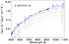 |
Fig. A.1. Observed X-SHOOTER spectrum of Apep Plume (in blue, 1Å sampling) overlaid with the best-fit model spectrum (in magenta) for the case of nominal distance of 2.4 kpc. The best-fit model spectra are calculated with CMFGEN using the mean model parameter values as given in Table A.1. The WC spectrum is in green colour, the WN spectrum is in red colour and the O spectrum is in black. |
We note that the derived stellar parameters of the massive stars responsible for the composite optical spectrum of Apep Plume can be considered within the norms for the respective spectral types (WC, WN, OB stars). Interestingly, the derived terminal velocities from our 4D grid-fitting using no a priori information are in acceptable correspondence with the values derived from the standard spectral analysis in the optical (so, no resonance lines): 2100 km s−1 (WC), 3500 km s−1 (WN), 1280 km s−1 (OB star) (Callingham et al. 2020).
As seen from Fig. A.1, it might seem a bit surprising that the optical emission of the OB star dominates the total composite spectrum (i.e. continuum) of Apep Plume. So, we performed the following technical check of this result.
Using the ancillary spectra (the 2D spectra) for each of the nine X-SHOOTER exposures of Apep Plume, we performed a fit in the cross-dispersion (i.e. in spatial) direction at certain wavelengths. We chose these wavelengths where the Apep Plume optical spectrum has no strong emission lines. In these fits, the model function consisted of two Gaussian components and a continuum. The fitting parameters were total flux and position of each component, the Gaussian width (being the same for both components) and the continuum level. The Gaussian components represent the two point sources of emission to be present: one for the central WC+WN binary, one for the northern OB star. Such fits were applied to each of the nine exposures as well as to the total 2D spectrum being the mean of the nine individual spectra.
Figure A.2 presents the result for the total 2D spectrum and we provide here the mean values of distance (separation) between the two point sources (in arcsec) : Δ = 0.74 (0.03) (at 6700Å), 0.72 (0.02) (at 7000Å), 0.73 (0.04) (at 8000Å), 0.73 (0.04) (at 9000Å). The values in parentheses are the standard deviation for the set of nine results (nine exposures). We note that the separation between the point sources is exactly as expected. We also see that the northern component is the stronger one as is found from our 4D grid-fitting to the total optical spectrum of Apep Plume.
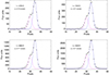 |
Fig. A.2. Examples of the spectral deconvolution using a model that is a sum of two Gaussians and underlying constant continuum. The data are depicted with filled diamonds. The fit components are shown with solid lines: the northern spectral component (OB star) in blue; the southern spectral component (WC+WN binary) in magenta. In each panel, shown are the wavelength the cross-dispersion cuts are taken at and the distance between the O and the WC+WN objects in arcseconds. |
Finally, we note that uncertainties of the distance to the studied object is one of the basic sources contributing to the inaccuracies of the stellar parameters derived from 4D-fitting of observed optical spectra, adopting stellar atmosphere models. While the wind velocity and stellar temperature do not depend on the distance, the other basic stellar parameters (mass-loss and luminosity) do depend strongly: Ṁ ∝ d1.5, L⋆ ∝ d2 (see Eqs. 1 and 4 from Hillier & Miller 1999).
On the one hand, we have to keep in mind that the situation in Apep Plume is a bit more complex since the distance to the OB star could be different from (larger than) the adopted distance of 2.4 kpc to Apep Plume. However, putting the OB star at larger distance will accordingly change the values of the derived mass-loss rate and luminosity for the OB star, while the spectrum level (flux density) will remain the same. In turn, the stellar parameters for the WC and WN stars will not be affected.
On the other hand, the actual distance to Apep Plume is still quite uncertain: there exist close by objects in the Gaia DR2 (Data Release 2) and DR3 (Data Release 3) catalogues but neither of them is yet associated with Apep Plume as seen from SIMBAD. As discussed already in Callingham et al. (2019), this might be a result from the multiplicity of this system and the presence of the complex extended dust circumstellar environment. But we only note that if one day we have a very accurate measurement of the distance to Apep Plume from Gaia and if its value puts this object close to us, say, at 600 pc, then this will require an appreciable decrease of the stellar luminosities derived in our analysis (e.g. by 1.2 dex). In turn, it will mean that the components in the central binary are unlikely to be WR stars: luminosities log L⋆ ≤ 4 (L⋆ in units of L⊙) are atypical for such massive stars. However, let us underline it again that before opening discussion (or start speculating) on a possible nature of Apep Plume in such a case, we first (and most importantly) need to have solid fact; that is, we need to have a very accurate measurement of the distance to this enigmatic object.
All Tables
All Figures
|
Fig. 1. Chandra images (0.5−10 keV) of Apep Plume (logarithmic intensity scale). RA (J2000) and Dec (J2000) are on the horizontal and vertical axes, respectively. The circled plus sign gives the near-infrared position of Apep Plume (SIMBAD). The asterisk gives the X-ray position derived by using the CIAO command WAVDETECT. |
| In the text | |
|
Fig. 2. Line profile fits to the He-like triplet of Fe XXV and the H-like doublets of S XVI and Si XIV in the first-order HETG spectra of Apep Plume. The spectra were rebinned for presentation purposes. |
| In the text | |
|
Fig. 3. Physical picture of CSWs in massive banaries. Left panel: Schematic presentation of the CSW region in massive WC+WN binary. The label CSW marks the wind interaction region, which is a 3D structure with its axis of symmetry Z. The axes X and Y complete the Cartesian coordinate system. The two angles i (orbital inclination) and α (azimuthal angle) define the orientation in space of the line of sight (l.o.s.) towards the observer. The label ‘Velocity’ denotes the general direction of the shocked plasma flow. The two dashed-line arrows illustrate that emission from a parcel of gas in the CSW region is subject to different wind absorption, depending on the orientation (i, α) of the l.o.s. towards the observer and the rotational angle around the axis of symmetry (Z). Right panel: CSW region derived from the 2D hydrodynamic simulations for the adopted values of the stellar-wind parameters in Apep Plume which give a wind-momentum rate ratio of the stellar winds of Λ = 4.86. The x- and z-axes are in units of the binary separation. The WC and WN components are located at (x, z) coordinates (0, 0) and (0, 1), respectively. The solid lines mark the shock fronts and the dashed line marks the contact discontinuity. The half opening angle of the WC shock (WC), contact discontinuity (CD), and the WN shock (WN) ‘cones’ is ∼47°, ∼64°, and ∼84°, respectively. |
| In the text | |
|
Fig. 4. Reduced χ2 values (degrees of freedom, d.o.f. = 343) as a function of partial heating at the shock fronts (β = Te/T) for the case of reduced mass-loss rates. The magenta circle marks the formal minimum value of the reduced χ2 at β = 0.6. |
| In the text | |
|
Fig. 5. The background-subtracted HETG (MEG – first row; HEG – second row) spectra of Apep Plume, overlaid with the best-fit model spectrum with β = 0.6. The spectra were rebinned to have a minimum of 20 counts per bin. |
| In the text | |
|
Fig. A.1. Observed X-SHOOTER spectrum of Apep Plume (in blue, 1Å sampling) overlaid with the best-fit model spectrum (in magenta) for the case of nominal distance of 2.4 kpc. The best-fit model spectra are calculated with CMFGEN using the mean model parameter values as given in Table A.1. The WC spectrum is in green colour, the WN spectrum is in red colour and the O spectrum is in black. |
| In the text | |
|
Fig. A.2. Examples of the spectral deconvolution using a model that is a sum of two Gaussians and underlying constant continuum. The data are depicted with filled diamonds. The fit components are shown with solid lines: the northern spectral component (OB star) in blue; the southern spectral component (WC+WN binary) in magenta. In each panel, shown are the wavelength the cross-dispersion cuts are taken at and the distance between the O and the WC+WN objects in arcseconds. |
| In the text | |
Current usage metrics show cumulative count of Article Views (full-text article views including HTML views, PDF and ePub downloads, according to the available data) and Abstracts Views on Vision4Press platform.
Data correspond to usage on the plateform after 2015. The current usage metrics is available 48-96 hours after online publication and is updated daily on week days.
Initial download of the metrics may take a while.