| Issue |
A&A
Volume 672, April 2023
|
|
|---|---|---|
| Article Number | A55 | |
| Number of page(s) | 8 | |
| Section | Extragalactic astronomy | |
| DOI | https://doi.org/10.1051/0004-6361/202245423 | |
| Published online | 30 March 2023 | |
Extended neutral hydrogen filamentary network in NGC 2403⋆
1
Netherlands Institute for Radio Astronomy (ASTRON), Oude Hoogeveensedijk 4, 7991 PD Dwingeloo, The Netherlands
e-mail: This email address is being protected from spambots. You need JavaScript enabled to view it.
2
Kapteyn Astronomical Institute, University of Groningen, PO Box 800, 9700 AV Groningen, The Netherlands
3
Department of Astronomy, University of Cape Town, Private Bag X3, 7701 Rondebosch, South Africa
4
Max Planck Institute for Astronomy, Königstuhl 17, 69117 Heidelberg, Germany
5
National Radio Astronomy Observatory, Pete V. Domenici Array Science Center, PO Box O Socorro, NM 87801, USA
Received:
10
November
2022
Accepted:
27
January
2023
Abstract
We present new neutral hydrogen (H I) observations of the nearby galaxy NGC 2403 to determine the nature of a low-column-density cloud that was detected earlier by the Green Bank Telescope. We find that this cloud is the tip of a complex of filaments of extraplanar gas that is coincident with the thin disk. The total H I mass of the complex is 2 × 10⁷ M⊙ or 0.6% of the total H I mass of the galaxy. The main structure, previously referred to as the 8 kpc filament, is now seen to be even more extended, along a 20 kpc stream. The kinematics and morphological properties of the filaments are unlikely to be the result of outflows related to galactic fountains. It is more likely that the 20 kpc filament is related to a recent galaxy interaction. In this context, a ∼50 kpc long stellar stream has recently been detected connecting NGC 2403 with the nearby dwarf satellite DDO 44. Intriguingly, the southern edge of this stream overlaps with the tip of the 20 kpc H I filament. We conclude that the H I anomalies in NGC 2403 are the result of a recent (∼2Gyr) interaction with DDO 44 leading to the observed filamentary complex.
Key words: galaxies: evolution / galaxies: interactions / techniques: interferometric / radio lines: galaxies
The reduced non-primary-beam-corrected datacube is also available at the CDS via anonymous ftp to cdsarc.cds.unistra.fr (130.79.128.5) or via https://cdsarc.cds.unistra.fr/viz-bin/cat/J/A+A/672/A55
© The Authors 2023
 Open Access article, published by EDP Sciences, under the terms of the Creative Commons Attribution License (https://creativecommons.org/licenses/by/4.0), which permits unrestricted use, distribution, and reproduction in any medium, provided the original work is properly cited.
This article is published in open access under the Subscribe to Open model. This email address is being protected from spambots. You need JavaScript enabled to view it. to support open access publication.
1. Introduction
Galaxies form stars through the collapsing of giant molecular (mainly molecular hydrogen, H2) clouds on timescales of ∼107 yr (Meidt et al. 2015; Schinnerer et al. 2019; Walter et al. 2020), and over cosmic time (Madau & Dickinson 2014) galaxies progressively deplete their molecular gas content. In a perfect steady state, the H2 reservoir is replenished by the cooling of the atomic hydrogen (H I) in the interstellar medium (Clark et al. 2012; Walch et al. 2015), which will cause a reduction in the content of the atomic gas. However, both simulations and observations reveal that the H I content in galaxies is almost constant from z ∼ 1 (Davé et al. 2017; Chen et al. 2021). Consequently, in order to maintain star formation over cosmic time, galaxies must accrete H I.
Previous studies of H I interaction features and dwarf galaxies have shown that these do not provide enough cold gas to replenish the material reservoir for star formation (Sancisi et al. 2008; Putman et al. 2012; de Blok et al. 2020). Other extraplanar gas observed closer to the galaxy disks is usually related to galactic fountains (Putman et al. 2012; Li et al. 2021; Marasco et al. 2022): star formation and supernova explosions eject interstellar medium from the disk to scale-heights of ∼1 kpc. The gas catches material from the circumgalactic medium and falls back onto the galaxy carrying new gas to fuel the star formation. However, the amount of material accreted with this process is again not enough to replenish the atomic gas reservoir (Putman et al. 2012; Afruni et al. 2021).
A hypothesis that could explain the constancy of the H I content is that galaxies accrete gas from the intergalactic medium (IGM; Somerville & Davé 2015; Danovich et al. 2015). The mode of this accretion, that is, cold clouds and streams or hot diffuse gas (Dekel & Birnboim 2006; Danovich et al. 2015), is uncertain, as is the accretion rate. Nevertheless, this model could indicate a possible way to solve the problem of how to sustain the star formation activities over cosmic time.
Nevertheless, it has one major limitation: the directly detectable component of this gas, namely the warm H I at ∼104 K, forms only a small fraction (< 1%) of the total amount of accreting material, which mostly consists of warm-hot 105 K gas. This leads to low H I column densities of ∼1017 cm−2 (Popping et al. 2009). This value is at least one order of magnitude lower than the detection limits of the current radio interferometer observations. Single-dish telescopes can reach these column densities but only at low resolutions that usually do not resolve the relevant scales. So far, surveys potentially able to detect accreting H I clouds have not found any direct evidence of them (Barnes et al. 2001; de Blok et al. 2002; Pisano et al. 2004; Giovanelli et al. 2007; Walter et al. 2008; Heald et al. 2011).
In this paper, we concentrate on one potential low-column-density cloud found with the Green Bank Telescope (GBT) near the well-studied spiral galaxy NGC 2403 (de Blok et al. 2014). The cloud is located ∼16 kpc (∼2R25) to the NW of the centre of the galaxy, but the low spatial resolution of the data prevents us from properly distinguishing it from the disk emission, meaning we are unable to robustly constrain its properties. The motivation behind this study is to confirm its detection with high-spatial-resolution radio interferometric data and to understand its nature; in particular, whether or not it is indeed the signature of the IGM accretion that previous studies have tried to find. With high-resolution data, we can also test other proposed scenarios, for example that it could be a result of strong outflow, or perhaps the remnant of a galactic interaction, and how it is linked to the kinematically anomalous H I features first detected by Fraternali et al. (2001). Additional analysis is presented in Fraternali et al. (2002), Fraternali & Binney (2006), Walter et al. (2008), de Blok et al. (2014).
NGC 2403 is a member of the M 81 group located at a distance of 3.18 Mpc (Madore & Freedman 1991) (1′=0.93 kpc, 1″ = 0.015 kpc) with a systemic velocity of 133.2 km s−1. The main H I disk is inclined by 63° and has a mass of 3.24 × 10⁹ M⊙. A list of these and other parameters can be found in Fraternali et al. (2002).
We obtained new H I radio observations of NGC 2403 and the GBT cloud in order to determine the nature of this cloud and explore its connection with the previously reported 8 kpc anomalous velocity filament (Fraternali et al. 2002).
In Sect. 2.1, we describe the data reduction and the creation of the data products that were analysed following the methods illustrated in Sect. 3. The main results and interpretation of our study are given in Sect. 4 and are summarised in Sect. 5.
2. Observations
The new Very Large Array (VLA) observations discussed in this paper were taken between December 5, 2019, and December 9, 2019, with the Expanded VLA in D-configuration1 (hereafter referred to as the 2019 data). The L-band bandwidth of 5.3 MHz comprised 2700 1.9 kHz (0.4 km s−1) channels with a central frequency of 1.41701 GHz. Two pointings were observed: 3 h centred on the galaxy (α = 7h36m44s, δ = 65° 35′35″) and another 3 h centred on the GBT cloud (α = 7h35m00s, δ = 65° 44′4″).
In addition to these new data, we also used archival VLA H I data of NGC 2403 centred on the galaxy. The archival data comprise The H I Nearby Galaxy Survey (THINGS) observations2 (Walter et al. 2008) and those discussed in Fraternali et al. (2001). Both data sets have a velocity resolution of 5.2 km s−1.
2.1. Data reduction
Here we give a brief description of the procedure used to reduce the new 2019 dataset. The data reduction was carried out with the software CASA v5.8.0 (McMullin et al. 2007). A preliminary data flagging was performed on the primary and secondary calibrator data (to correct for shadowing, correlator glitches, misbehaving antennas, bandwidth cut-offs, radio frequency interference (RFI), Milky Way emission, and absorption) as well as on NGC 2403 (to take into account shadowing, correlator glitches, and misbehaving antennas) with the CASA task flagdata. The RFI was manually removed in CASA plotms. A calibration model was then built with the following corrections: target elevation, delay, bandpass, complex gain, and flux scale using the CASA tasks gencal, gaincal, and fluxscale. A set of weights for the data was constructed based on the variance of the data with the CASA task statwt and a Hanning-smoothing in frequency was applied to remove Gibbs ringing artefacts with the CASA task hanningsmooth. Finally, the continuum was estimated with a simple linear fit – which is justified by the narrow band width – to the amplitudes and phases in the line-free channels and subtracted from the data with the CASA task uvcontsub. The THINGS and the 1999 data were re-reduced using similar standard procedures.
2.2. Cube creation
We used the CASA task tclean to create a combined mosaicked H I cube of the two pointings of the 2019 data. We applied a robustness parameter of 0.5 and a tapering of 48″ to the data in order to balance spatial resolution and sensitivity. Choosing a pixel size of 9″ to properly sample the beam, and accounting for the primary beam size then yielded channel maps with an extent of 400 × 400 pixels. As our aim is to combine the new observations with the archival data, we chose the channel width to be 5.3 km s−1, leading to 209 channels covering the range −377.8 to 724.6 km s−1.
tclean was run in the auto-multithresh masking mode: for each iteration of the cleaning process and for each channel of the cube, a mask was created that enclosed the emission above 4 × σ in the channel. Inside the masked region, tclean smooths the data by a factor of 1.5 and cleans until it reaches the stopping threshold of 0.5σ, where the noise is now that of the smoothed channel. This results in a cube based on only the new data.
In addition, we used tclean to combine all the available observations including the archival data into a single H I cube and used the same imaging parameters as the mosaicked 2019 cube above. As the different uv distributions in the two pointings would lead to different resolutions over the mosaic, we applied a 48″ taper, which resulted in a common beam size for the entire mosaic. Furthermore, the noise is different for the two pointings, but at every position the mosaic has the highest signal-to-noise ratio possible given the data. We return to this topic below. The more limited velocity range of the archival data resulted in a cube with 102 channels of 5.3 km s−1.
3. Data analysis
3.1. Cube statistics
Throughout this paper, the given noise values are referring to the non-primary-beam-corrected cubes, while all the flux density and H I mass measurements were performed on primary-beam-corrected data. The 2019 H I cube has a beam size of 62 × 55arcsec (1.24 × 1.1 kpc) and the single-channel median noise is σ = 0.53mJy beam−1. This can be converted into an H I column density with the equation
 (1)
(1)
where F is the flux density in Jy beam−1, Δv is the velocity width in km s−1, and A is the beam area in arcsec2 calculated assuming a Gaussian beam: A = 1.13ab, where a and b are the beam major and minor axis in arcsec, respectively. The resulting 3σ one-channel column density is 2.7 × 1018 cm−2.
The H I cube that also includes the archival data has a beam size of 52 × 49 arcsec (1.04 × 0.98 kpc). The noise in this cube is not spatially constant due to the combination of different pointings with different integration times. The median σ in the NW pointing is 0.31 mJy beam−1, while in the central pointing it is 0.23 mJy beam−1. Adopting the median noise value across the mosaic of σ = 0.295 mJy beam−1, gives a 3σ one-channel H I column density of 2 × 1018 cm−2, as an indicative sensitivity for the combined cube.
3.2. H I detections
As the cube resulting from the combination of the new and archival data has lower noise, we use it to create the detection mask by running the H I Source Finding Application (SoFiA2) v2.4.0 (Serra et al. 2015; Westmeier et al. 2021). SoFiA2 internally corrects for the uneven noise, so the flux threshold (expressed in multiples of the noise level) for detecting emission is consistent across the field. We blanked the channels from −55 km s−1 to 5 km s−1 as they contain strong Milky Way contamination, and used SoFiA2 to identify the emission in the data cube using the S+C method. We used a spatial kernel equal to zero, one, and two times the beam size (i.e., a kernel of 0 × 0, 3.1 × 3.1 and 6.2 × 6.2 pixels) and a spectral kernel equal to 0, 3, and 7 channels, a detection threshold of 3σ, and a reliability threshold of 0.95.
We produced also the moment-zero, -one, and -two maps by setting the linker in SoFiA2 to be a 1 × 1 × 1 box (1 × 1 pixel and 1 channel) and by rejecting all the sources whose size is less than 6 × 6 × 3 (6 × 6 pixel and 3 channels). The moment maps are given in Fig. 1. We calculated an H I mass for the galaxy of 3.2 × 10⁹ M⊙, which agrees with previous radio interferometric measurements (Fraternali et al. 2002; Walter et al. 2008).
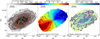 |
Fig. 1. NGC 2403 moment maps. Left panel: primary-beam-corrected H I column-density map of NGC 2403 with reversed grey-scale colour map from faint (grey) to bright (black) emission. The sharp cut-off in the bottom left is due to the 20% cut-off threshold of the primary beam response, which is illustrated with the light grey curve. The contours levels are (5, 75, 200, 500, 1000, 2000) × 1018 cm−2. The column density limit 3 × σ × dv = 2 × 1018 cm−2, where dv = 5.3 km s−1 is the spectral resolution, is reported at the bottom. In the bottom right we show the 52″ × 49″ beam. Central panel: intensity-weighted mean velocity field of NGC 2403 with respect to the systemic velocity of 133.2 km s−1, given at the bottom. Dashed contours (−105, −70, −35) km s−1 refer to the approaching side, while solid lines correspond to radial velocities of (35, 70, 105) km s−1. The thick grey line is the kinematical minor axis. Right panel: second moment map, where the signature of the filaments with their anomalous velocities is visible in the increased second-moment values. |
Figure 2 shows the channel maps covering the velocity range over which H I emission is found. From now on, all the velocity values are given relative to the systemic velocity of 133.2 km s−1. Apart from the well-known 8 kpc filament (Fraternali et al. 2002; de Blok et al. 2014), we indicate three additional filamentary structures, pointed out in Fig. 2 with the arrows: (1) between −59 km s−1 and −27 km s−1 on the east side (red arrow in Fig. 2); (2) from −27 km s−1 to 15 km s−1 on the west side of the galaxy (blue arrow in Fig. 2) next to the 8 kpc filament; and (3) from 15 km s−1 to 47 km s−1 on the west side of the galaxy (green arrow in Fig. 2) above the 8 kpc filament. The 8 kpc filament found in previous work may be part of a more extended H I stream as clearly shown in the 15 km s−1 channel, whose total extent is at least 20 kpc. We denote this the ‘20 kpc filament’ or ‘main filament’. The high-column-density parts of the other two structures were previously detected by Fraternali et al. (2001), but the increased column-density sensitivity of the new data presented here highlights their filamentary shape and extent.
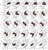 |
Fig. 2. NGC 2403 H I channel maps of the data cube with both new and archival observations where we show only every second channel. The colour-scale contours correspond to 2 × (1, 4, 16, 64) × 1018 cm−2, where 2 × 1018 cm−2 is the 3σ one-channel column density limit. The thick contour levels indicate the significant emission identified by the SoFiA source finder. Most of the low-level structures shown in thin contours are noise or mosaicking artefacts. The dashed grey contours denote the column density of −2 × 1018 cm−2. The egg-shaped borders are due to the 20% cut-off threshold of the primary beam response. At the bottom, we report the line-of-sight velocity (with respect to the systemic velocity 133.2 km s−1) in each channel. The filamentary detections, labelled with coloured arrows, are evident between −59 km s−1 and 47 km s−1. |
The location of the above features in velocity space implies that they are not co-rotating with the thin disk. It is therefore possible to kinematically isolate them from the thin disk emission for a detailed study.
3.3. Extraction of the H I filaments
As a first step, we isolate the thin disk following the method presented in Fraternali et al. (2002). We fit a single Gaussian to the line profile for each position in the sky, resulting in a ‘Gaussian cube’, which we subtract from the data cube.
We then used the velocities of the peak values of these fitted profiles to line up all H I emission profiles for each position on the sky at their peak velocities. This method is called ‘shuffle’ and was applied to both the cube and the SoFiA2 detection mask produced as described above; it is a powerful tool to easily isolate the anomalous velocity gas, for example as a function of the deviation from the thin disk rotation as shown in Fig. 3. Here, the gas rotating with the disk occupies the central channels of the shuffled cube, while H I that is not rotating with the disk will be placed at higher or lower channels. Hence, the non-co-rotating gas can be easily identified, as we show in Fig. 3.
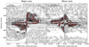 |
Fig. 3. Position–velocity diagram along the major axis (left panel) and minor axis (right panel) through a beam-wide slice of the shuffled data cube without the thin-disk removal. The emission is mapped with a reverse grey scale and we overlaid the 2 × (1, 3, 9) × 1018 cm−2 levels with grey-scale contours. The blanked area in the top left and blank stripe in the bottom are the result of the Milky Way filtering. The grey dashed lines denote the column density of −3σ. The channels between ±65 km s−1 with the residual thin disk and diffuse extraplanar emission are highlighted with the hatched area; they were not used for the computation of the moment map shown in the central panel of Fig. 4. |
We isolated the channels of the shuffled cube where the filamentary emission is present by blanking the channels between ±65 km s−1 (or equivalently ±14 times the full width at half maximum of the disk profiles). This selection is conservative by design. Our aim is to isolate the filaments with the highest velocities that are most likely not associated with the thin disk or the thicker and lagging disk as identified in Fraternali et al. (2002). A narrower velocity cut than used here would include a significant amount of gas from this lagging, thick disk. We calculated the moment maps of the anomalous-velocity gas using the shuffled detection mask. The result is given in Fig. 4, where we show the overlay between the galaxy emission and the GBT detection (left panel), the filamentary complex (central panel), and the selection effect introduced by the shuffle procedure (right panel), which we discuss in the following section.
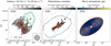 |
Fig. 4. Left panel: primary-beam-corrected H I column density map of NGC 2403 (in reverse grey-scale colourmap) overlaid with the GBT cloud candidate (green) from de Blok et al. (2014). The map was produced by integrating over the channels from −22 km s−1 to 20 km s−1 with respect to the systemic velocity. This range corresponds to the one used by de Blok et al. (2014) to compute the candidate GBT cloud moment-zero map. Grey-scale contour levels are from 5 × 1018 cm−2 to 1 × 1021 cm−2. The 3σ one-channel column-density limit is reported at the bottom. The beam of the interferometric data for both the GBT and our VLA observations is shown in the bottom right. The green contours instead define the (6.25, 12.5, 25, 62.5) – 1017 cm−2 column density in the GBT data. The light-grey line denotes the 20% cut-off threshold of the primary beam response. Central panel: primary-beam-corrected H I column-density map of the anomalous-velocity gas. Grey-scale contour levels are (3, 10, 25, 50, 100) × 1018 cm−2 column density. The spatial scale is the same as in the left panel, and the light grey line shows the same cut-off threshold. We indicate the galaxy edge with the dashed-black contour. The light blue dashed line represents the path along which the position-velocity slice has been extracted (see Fig. 5). Right panel: illustrative example of the selection effect introduced by the shuffle procedure (see discussion in Sect. 4). The map shows the fraction of the original extraplanar flux density of a mock galaxy we were able to recover and the red contour encloses the region where we are severely affected by selection effect, i.e., where more than 90% of the original flux density is lost. The blanked bits in the centre denote the region where the result is unreliable because of the steep gradient in velocity. The dashed white contours indicate the region occupied by the observed filamentary complex. |
4. Discussion
The H I filaments have a total mass of at least 2.0 × 10⁷ M⊙, about 0.6% of the total H I mass of the galaxy. This is a lower limit, firstly because of the chosen channel cut at ±65 km s−1, and secondly because close to the kinematical minor axis of the galaxy, any anomalous velocity gas co-rotating or counter-rotating with the disk will not be distinguishable. In other words, as we look close to the kinematical minor axis, the line profile of the thin disk and of the extraplanar gas overlap more and more, and we are not able to distinguish between thin disk and co-rotating or counter-rotating anomalous velocity gas.
We used the following simple model to estimate the importance of this effect: we built a mock galaxy with a thin (dispersion of 10 km s−1) disk and a thick (dispersion of 35 km s−1) disk which rotates 30 km s−1 slower and has a column density equal to 10% of the thin disk. These parameters are modelled on the properties of NGC 2403 as described in Fraternali et al. (2002).
We repeated the same steps with the observed data (Gaussian fit, thin-disk removal, shuffle, and blanking of all the channels between ±65 km s−1) in order to check how our ability to extract the anomalous H I varies as a function of the position angle along the disk. We do indeed find that the ability to separate the anomalous velocity gas from the thin disk changes with position angle. In the right panel of Fig. 4 we illustrate the effect.
The projected extent of the filaments varies from ∼10 kpc up to ∼20 kpc, and they are almost aligned with the galactic major axis. This is not purely a result of selection effects, as the distribution of the observed anomalous H I in the right panel of Fig. 4 clearly shows.
The GBT cloud found by de Blok et al. (2014) is at the location of the tip of the 20 kpc filament and can possibly be identified with it; this feature resembles a cloud in the GBT data simply because of the very low spatial resolution of these data and the limited velocity range over which it could be identified.
The larger extension of the main filament – as visible in the new data due to the increased sensitivity – is shown in Fig. 5, where we show the position–velocity diagram along the main filament and the cloud compared to the same position velocity slice presented in Fig. 6 in de Blok et al. (2014).
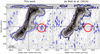 |
Fig. 5. Comparison between the position–velocity diagram through the centres of the cloud candidate and the 20 kpc filament along a 100″-thick slice as taken through our data (left panel) and as shown in Fig. 6 in de Blok et al. (2014) (right panel). The emission is mapped with a reverse grey scale and we overlaid the 2.5 × (1, 9, 81) × 1018 cm−2 column density levels with colour-scale contours (black, red and white, respectively). The blue contour denotes a level of 1.2 × 1018 cm−2 and highlights the detection of the 20 kpc filament tip with the combination of the new and archival VLA data. The red circles highlight the tip of the 20 kpc filament which was not detected in the Fraternali et al. (2002) and de Blok et al. (2014) analyses. |
In the following, we further discuss the possible origins of this filamentary complex.
4.1. Confirmation of the GBT cloud
The motivation of this study was to confirm the GBT detection of an H I cloud near NGC 2403 (de Blok et al. 2014) and to understand its origin. The left panel of Fig. 4 shows that the GBT cloud overlaps with the northern part of the 20 kpc filament. Indeed, the column density of the gas in the northern region of the filament is > 1018 cm−2 at the spatial resolution of ∼50 arcsec and de Blok et al. (2014) estimate an average column density of 2.4 × 1018 cm−2 for the cloud. Therefore, the tip of the 20 kpc filament could have been seen by the GBT.
The H I mass of the cloud as measured with the GBT is 6.3 × 10⁶ M⊙, while the H I content within the GBT contours in our data is 1.2 × 10⁶ M⊙. Given the inherent difficulty in separating the cloud and disk emission in the GBT data and the conservative blanking criteria used to extract the filamentary emission in our shuffle cube, this must be regarded as reasonable agreement and thus further supports the identification of the GBT cloud with the northern tip of the filament detected by the VLA.
4.2. The nature of the 20 kpc filament
One of the questions we try to answer is whether the GBT cloud, and by implication the filaments described in this paper, are formed due to a gas-accretion event. However, there are other possible explanations for these features, some of which we have already briefly alluded to. For example, the structures we observe could be the result of a galactic fountain process that ejects gas from the disk. This is certainly a likely scenario for the anomalous velocity gas closer to the disk (i.e., below our ±65 km s−1 cut-off), but the situation is less clear for the filaments.
It is difficult to form a straight 20 kpc-long filament in an outflow scenario. Indeed, in a pure galactic fountain model the gas ejecta reaches distances of at most 10 kpc even with extremely high kick velocities (Fraternali & Binney 2006, 2008).
The origin of the filamentary complex could still be galactic interaction. In the event of a merging or disrupting dwarf, one might expect to see a disturbed stellar population from the dwarf, most likely coinciding with or near the filaments. Barker et al. (2012) performed an in-depth study of the stellar properties in NGC 2403 but did not identify any peculiarities in the distribution of the stars and concluded that the galaxy has evolved in isolation with no significant recent merging event.
However, their Fig. 10 shows some evidence for a slightly disturbed stellar component in the NW part of the disk. These authors also reported an extended low-metallicity red giant branch (RGB) component at radii between 18 and 40 kpc. Their interpretation includes the presence of a stellar halo, or a thick stellar disk in NGC 2403, but it is not clear whether this component is associated with an accretion or interaction event.
In de Blok et al. (2014) it was shown that a line passing through the major axis of the 8 kpc filament and the GBT cloud intersects with nearby dwarf galaxies DDO 44 and NGC 2366, hinting at a possible interaction scenario with either of these galaxies. Recent deep optical wide-field data presented in Carlin et al. (2019) support this idea. These authors observed a ∼50 kpc long stellar stream originating from the dwarf galaxy DDO 44 and connecting with the NW part of the stellar disk of NGC 2403. This dwarf is likely a satellite of NGC 2403 located about 70 kpc from it. A higher-quality re-reduction of the data from Carlin et al. (2019) is given in Fig. 6 (Carlin, priv. comm) and this shows the stellar stream and the connection between DDO 44 and NGC 2403 even more clearly.
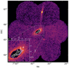 |
Fig. 6. Overlay of the re-reduced density map of candidate RGB stars presented in Carlin et al. (2019) and the H I filaments observed in our data (white contours). Bins in the density map are completeness-corrected and have a resolution of 0.75 arcmin. The hole in the centre is due to extreme crowding. The colours denote the number of stars per 0.75′ bin. The stellar stream is connecting DDO 44 and NGC 2403 with the tip of the H I filaments, strongly suggesting that DDO 44 and NGC 2403 recently underwent an interaction. |
This image is a 1.5° wide-field composite mosaic of seven pointings taken with the Hyper Suprime-Cam of the 8.2 m Subaru Telescope and converted into a density map of candidate RGB stars. Overlaid on that map, we show the filamentary H I. There is a remarkable coincidence between the position of the tip of the 20 kpc filament and the region where the DDO 44 stellar stream connects with NGC 2403 stellar disk. This is therefore a strong indication that the dwarf interaction scenario can be responsible for the H I filaments in NGC 2403.
This is also suggested by the star formation histories of the galaxies: NGC 2403 had an increase in its star formation rate about 2 Gyr ago (Williams et al. 2013), in particular at radii > 20 kpc; while DDO 44 had a burst of star formation from 1 to 3 Gyr ago (Girardi et al. 2010; Weisz et al. 2011). Also, Carlin et al. (2019) calculated from the estimated trajectory of DDO 44 that the interaction with NGC 2403 occurred ∼1 Gyr ago. These various estimates therefore give very similar timescales for the interaction.
The most likely explanation is therefore that the H I filaments in NGC 2403 are the result of the interaction with DDO 44. Nevertheless, this does not preclude a galactic fountain scenario as a potential origin for a part of the extraplanar gas in NGC 2403, especially for the gas at less extreme velocities than the filaments. It is interesting to note that for two of the most well-known nearby galaxies where extraplanar filaments are prominent, NGC 2403 and NGC 891, an interaction scenario is now the most likely cause (see Oosterloo et al. 2007 for the NGC 891 analysis).
5. Conclusion
Using new and archival VLA observations, we present a study of NGC 2403, focusing on the nature of the GBT cloud (de Blok et al. 2014). These data show a filamentary complex around the galaxy with an H I mass of 2.0 × 10⁷ M⊙. This complex is comprised of at least three filaments of 10–20 kpc in length. The GBT cloud can now be shown to be the tip of the longest structure.
Even though at first sight the stellar distribution in NGC 2403 appears undisturbed, it is now likely that these filaments are the result of an interaction with a nearby dwarf galaxy. Hints of a disturbance in the stellar component were already visible in the data presented in Barker et al. (2012), but they were dramatically confirmed in the recent study by Carlin et al. (2019), who discovered a ∼50 kpc long stellar stream connecting DDO 44 and NGC 2403. The intersection of that stream with NGC 2403 coincides with the positions of the tip of the H I filaments. The star formation history of the two galaxies and the estimated trajectory of DDO 44 seem to suggest that the interaction occurred about 1 Gyr ago.
These observations highlight the importance of minor interactions in shaping the H I disks of galaxies. Moreover, they point out the difficulty in unambiguously identifying the effects of direct cold-gas accretion from the IGM, and distinguishing them from those of minor interactions with a satellite. In this regard, the multi-wavelength approach is fundamental: optical observations are crucial to provide solid evidence for accretion or interaction as the most plausible explanation of anomalous H I structures such as the filaments.
Future observations with the SKA and its precursors at higher resolution and higher sensitivity will undoubtedly uncover many more of these features in nearby galaxies and will help us to better understand how the balance between accretion and interaction impacts the evolution of galaxies.
Project ID: 19B-081.
We included the data from the C- and D-array configurations only.
Acknowledgments
We would like to thank A. Fergusson for providing us with the stellar catalogue from Barker et al. 2012. We thank F. Fraternali for the useful discussions about the interpretation of our results and F. Maccagni for the initial discussions on the DDO 44 optical data. A. Marasco’s help in the modelling of our data is gratefully acknowledged. Also, we thank J. Carlin for kindly sharing with us the new re-reduced optical data of DDO 44. We thank the anonymous referee for the constructive comments and the suggested improvements for the quality and clarity of this paper. This work has received funding from the European Research Council (ERC) under the European Union’s Horizon 2020 research and innovation programme (grant agreement No 882793 ‘MeerGas’).
References
- Afruni, A., Fraternali, F., & Pezzulli, G. 2021, MNRAS, 501, 5575 [NASA ADS] [Google Scholar]
- Barker, M. K., Ferguson, A. M. N., Irwin, M. J., Arimoto, N., & Jablonka, P. 2012, MNRAS, 419, 1489 [CrossRef] [Google Scholar]
- Barnes, D. G., Staveley-Smith, L., de Blok, W. J. G., et al. 2001, MNRAS, 322, 486 [Google Scholar]
- Carlin, J. L., Garling, C. T., Peter, A. H. G., et al. 2019, ApJ, 886, 109 [NASA ADS] [CrossRef] [Google Scholar]
- Chen, Q., Meyer, M., Popping, A., et al. 2021, MNRAS, 508, 2758 [NASA ADS] [CrossRef] [Google Scholar]
- Clark, P. C., Glover, S. C. O., Klessen, R. S., & Bonnell, I. A. 2012, MNRAS, 424, 2599 [CrossRef] [Google Scholar]
- Danovich, M., Dekel, A., Hahn, O., Ceverino, D., & Primack, J. 2015, MNRAS, 449, 2087 [Google Scholar]
- Davé, R., Rafieferantsoa, M. H., Thompson, R. J., & Hopkins, P. F. 2017, MNRAS, 467, 115 [NASA ADS] [Google Scholar]
- de Blok, W. J. G., Zwaan, M. A., Dijkstra, M., Briggs, F. H., & Freeman, K. C. 2002, A&A, 382, 43 [NASA ADS] [CrossRef] [EDP Sciences] [Google Scholar]
- de Blok, W. J. G., Keating, K. M., Pisano, D. J., et al. 2014, A&A, 569, A68 [NASA ADS] [CrossRef] [EDP Sciences] [Google Scholar]
- de Blok, W. J. G., Athanassoula, E., Bosma, A., et al. 2020, A&A, 643, A147 [NASA ADS] [CrossRef] [EDP Sciences] [Google Scholar]
- Dekel, A., & Birnboim, Y. 2006, MNRAS, 368, 2 [NASA ADS] [CrossRef] [Google Scholar]
- Fraternali, F., & Binney, J. J. 2006, MNRAS, 366, 449 [CrossRef] [Google Scholar]
- Fraternali, F., & Binney, J. J. 2008, MNRAS, 386, 935 [CrossRef] [Google Scholar]
- Fraternali, F., Oosterloo, T., Sancisi, R., & van Moorsel, G. 2001, ApJ, 562, L47 [CrossRef] [Google Scholar]
- Fraternali, F., van Moorsel, G., Sancisi, R., & Oosterloo, T. 2002, AJ, 123, 3124 [CrossRef] [Google Scholar]
- Giovanelli, R., Haynes, M. P., Kent, B. R., et al. 2007, AJ, 133, 2569 [NASA ADS] [CrossRef] [Google Scholar]
- Girardi, L., Williams, B. F., Gilbert, K. M., et al. 2010, ApJ, 724, 1030 [NASA ADS] [CrossRef] [Google Scholar]
- Heald, G., Józsa, G., Serra, P., et al. 2011, A&A, 526, A118 [NASA ADS] [CrossRef] [EDP Sciences] [Google Scholar]
- Li, A., Marasco, A., Fraternali, F., Trager, S., & Verheijen, M. A. W. 2021, MNRAS, 504, 3013 [NASA ADS] [CrossRef] [Google Scholar]
- Madau, P., & Dickinson, M. 2014, ARA&A, 52, 415 [Google Scholar]
- Madore, B. F., & Freedman, W. L. 1991, PASP, 103, 933 [Google Scholar]
- Marasco, A., Fraternali, F., Lehner, N., & Howk, J. C. 2022, MNRAS, 515, 4176 [NASA ADS] [CrossRef] [Google Scholar]
- McMullin, J. P., Waters, B., Schiebel, D., Young, W., & Golap, K. 2007, in Astronomical Data Analysis Software and Systems XVI, eds. R. A. Shaw, F. Hill, & D. J. Bell, ASP Conf. Ser., 376, 127 [Google Scholar]
- Meidt, S. E., Hughes, A., Dobbs, C. L., et al. 2015, ApJ, 806, 72 [NASA ADS] [CrossRef] [Google Scholar]
- Oosterloo, T., Fraternali, F., & Sancisi, R. 2007, AJ, 134, 1019 [Google Scholar]
- Pisano, D. J., Barnes, D. G., Gibson, B. K., et al. 2004, ApJ, 610, L17 [NASA ADS] [CrossRef] [Google Scholar]
- Popping, A., Davé, R., Braun, R., & Oppenheimer, B. D. 2009, A&A, 504, 15 [NASA ADS] [CrossRef] [EDP Sciences] [Google Scholar]
- Putman, M. E., Peek, J. E. G., & Joung, M. R. 2012, ARA&A, 50, 491 [Google Scholar]
- Sancisi, R., Fraternali, F., Oosterloo, T., & van der Hulst, T. 2008, A&ARv, 15, 189 [NASA ADS] [CrossRef] [Google Scholar]
- Schinnerer, E., Hughes, A., Leroy, A., et al. 2019, ApJ, 887, 49 [NASA ADS] [CrossRef] [Google Scholar]
- Serra, P., Westmeier, T., Giese, N., et al. 2015, MNRAS, 448, 1922 [Google Scholar]
- Somerville, R. S., & Davé, R. 2015, ARA&A, 53, 51 [Google Scholar]
- Walch, S., Girichidis, P., Naab, T., et al. 2015, MNRAS, 454, 238 [Google Scholar]
- Walter, F., Brinks, E., de Blok, W. J. G., et al. 2008, AJ, 136, 2563 [Google Scholar]
- Walter, F., Carilli, C., Neeleman, M., et al. 2020, ApJ, 902, 111 [Google Scholar]
- Weisz, D. R., Dalcanton, J. J., Williams, B. F., et al. 2011, ApJ, 739, 5 [CrossRef] [Google Scholar]
- Westmeier, T., Kitaeff, S., Pallot, D., et al. 2021, MNRAS, 506, 3962 [NASA ADS] [CrossRef] [Google Scholar]
- Williams, B. F., Dalcanton, J. J., Stilp, A., et al. 2013, ApJ, 765, 120 [NASA ADS] [CrossRef] [Google Scholar]
All Figures
|
Fig. 1. NGC 2403 moment maps. Left panel: primary-beam-corrected H I column-density map of NGC 2403 with reversed grey-scale colour map from faint (grey) to bright (black) emission. The sharp cut-off in the bottom left is due to the 20% cut-off threshold of the primary beam response, which is illustrated with the light grey curve. The contours levels are (5, 75, 200, 500, 1000, 2000) × 1018 cm−2. The column density limit 3 × σ × dv = 2 × 1018 cm−2, where dv = 5.3 km s−1 is the spectral resolution, is reported at the bottom. In the bottom right we show the 52″ × 49″ beam. Central panel: intensity-weighted mean velocity field of NGC 2403 with respect to the systemic velocity of 133.2 km s−1, given at the bottom. Dashed contours (−105, −70, −35) km s−1 refer to the approaching side, while solid lines correspond to radial velocities of (35, 70, 105) km s−1. The thick grey line is the kinematical minor axis. Right panel: second moment map, where the signature of the filaments with their anomalous velocities is visible in the increased second-moment values. |
| In the text | |
|
Fig. 2. NGC 2403 H I channel maps of the data cube with both new and archival observations where we show only every second channel. The colour-scale contours correspond to 2 × (1, 4, 16, 64) × 1018 cm−2, where 2 × 1018 cm−2 is the 3σ one-channel column density limit. The thick contour levels indicate the significant emission identified by the SoFiA source finder. Most of the low-level structures shown in thin contours are noise or mosaicking artefacts. The dashed grey contours denote the column density of −2 × 1018 cm−2. The egg-shaped borders are due to the 20% cut-off threshold of the primary beam response. At the bottom, we report the line-of-sight velocity (with respect to the systemic velocity 133.2 km s−1) in each channel. The filamentary detections, labelled with coloured arrows, are evident between −59 km s−1 and 47 km s−1. |
| In the text | |
|
Fig. 3. Position–velocity diagram along the major axis (left panel) and minor axis (right panel) through a beam-wide slice of the shuffled data cube without the thin-disk removal. The emission is mapped with a reverse grey scale and we overlaid the 2 × (1, 3, 9) × 1018 cm−2 levels with grey-scale contours. The blanked area in the top left and blank stripe in the bottom are the result of the Milky Way filtering. The grey dashed lines denote the column density of −3σ. The channels between ±65 km s−1 with the residual thin disk and diffuse extraplanar emission are highlighted with the hatched area; they were not used for the computation of the moment map shown in the central panel of Fig. 4. |
| In the text | |
|
Fig. 4. Left panel: primary-beam-corrected H I column density map of NGC 2403 (in reverse grey-scale colourmap) overlaid with the GBT cloud candidate (green) from de Blok et al. (2014). The map was produced by integrating over the channels from −22 km s−1 to 20 km s−1 with respect to the systemic velocity. This range corresponds to the one used by de Blok et al. (2014) to compute the candidate GBT cloud moment-zero map. Grey-scale contour levels are from 5 × 1018 cm−2 to 1 × 1021 cm−2. The 3σ one-channel column-density limit is reported at the bottom. The beam of the interferometric data for both the GBT and our VLA observations is shown in the bottom right. The green contours instead define the (6.25, 12.5, 25, 62.5) – 1017 cm−2 column density in the GBT data. The light-grey line denotes the 20% cut-off threshold of the primary beam response. Central panel: primary-beam-corrected H I column-density map of the anomalous-velocity gas. Grey-scale contour levels are (3, 10, 25, 50, 100) × 1018 cm−2 column density. The spatial scale is the same as in the left panel, and the light grey line shows the same cut-off threshold. We indicate the galaxy edge with the dashed-black contour. The light blue dashed line represents the path along which the position-velocity slice has been extracted (see Fig. 5). Right panel: illustrative example of the selection effect introduced by the shuffle procedure (see discussion in Sect. 4). The map shows the fraction of the original extraplanar flux density of a mock galaxy we were able to recover and the red contour encloses the region where we are severely affected by selection effect, i.e., where more than 90% of the original flux density is lost. The blanked bits in the centre denote the region where the result is unreliable because of the steep gradient in velocity. The dashed white contours indicate the region occupied by the observed filamentary complex. |
| In the text | |
|
Fig. 5. Comparison between the position–velocity diagram through the centres of the cloud candidate and the 20 kpc filament along a 100″-thick slice as taken through our data (left panel) and as shown in Fig. 6 in de Blok et al. (2014) (right panel). The emission is mapped with a reverse grey scale and we overlaid the 2.5 × (1, 9, 81) × 1018 cm−2 column density levels with colour-scale contours (black, red and white, respectively). The blue contour denotes a level of 1.2 × 1018 cm−2 and highlights the detection of the 20 kpc filament tip with the combination of the new and archival VLA data. The red circles highlight the tip of the 20 kpc filament which was not detected in the Fraternali et al. (2002) and de Blok et al. (2014) analyses. |
| In the text | |
|
Fig. 6. Overlay of the re-reduced density map of candidate RGB stars presented in Carlin et al. (2019) and the H I filaments observed in our data (white contours). Bins in the density map are completeness-corrected and have a resolution of 0.75 arcmin. The hole in the centre is due to extreme crowding. The colours denote the number of stars per 0.75′ bin. The stellar stream is connecting DDO 44 and NGC 2403 with the tip of the H I filaments, strongly suggesting that DDO 44 and NGC 2403 recently underwent an interaction. |
| In the text | |
Current usage metrics show cumulative count of Article Views (full-text article views including HTML views, PDF and ePub downloads, according to the available data) and Abstracts Views on Vision4Press platform.
Data correspond to usage on the plateform after 2015. The current usage metrics is available 48-96 hours after online publication and is updated daily on week days.
Initial download of the metrics may take a while.