| Issue |
A&A
Volume 672, April 2023
|
|
|---|---|---|
| Article Number | A179 | |
| Number of page(s) | 12 | |
| Section | Extragalactic astronomy | |
| DOI | https://doi.org/10.1051/0004-6361/202245247 | |
| Published online | 19 April 2023 | |
AGN feedback in an infant galaxy cluster: LOFAR-Chandra view of the giant FRII radio galaxy J103025+052430 at z = 1.7
1
INAF – Osservatorio di Astrofisica e Scienza dello Spazio di Bologna, Via P. Gobetti 93/3, 40129 Bologna, Italy
e-mail: This email address is being protected from spambots. You need JavaScript enabled to view it.
2
Dipartimento di Fisica e Astronomia, Universiti di Bologna, via P. Gobetti 93/2, 40129 Bologna, Italy
3
INAF – Istituto di Radioastronomia, Bologna Via Gobetti 101, 40129 Bologna, Italy
4
SISSA, Via Bonomea 265, 34136 Trieste, Italy
5
Harvard-Smithsonian Center for Astrophysics, 60 Garden Street, Cambridge, MA 02138, USA
6
The William H. Miller III Department of Physics & Astronomy, Johns Hopkins University, Baltimore, MD 21218, USA
7
Space Telescope Science Institute for the European Space Agency, ESA Office, 3700 San Martin Drive, Baltimore, MD 21218, USA
8
Institut de Ciències del Cosmos (ICCUB), Universitat de Barcelona (IEEC-UB), Martí i Franquès, 1, 08028 Barcelona, Spain
9
ICREA, Pg. Lluís Companys 23, 08010 Barcelona, Spain
10
Department of Physics and Astronomy, Clemson University, Kinard Lab of Physics, Clemson, SC 29634, USA
11
Leiden Observatory, Leiden University, PO Box 9513 2300 RA Leiden, The Netherlands
12
Department of Physics, University of Miami, Coral Gables, FL 33124, USA
13
INAF – Osservatorio Astrofisico di Catania, Catania Via Santa Sofia 78, 95123 Catania, Italy
14
ASTRON, Netherlands Institute for Radio Astronomy, Oude Hoogeveensedijk 4, 7991 PD Dwingeloo, The Netherlands
15
INAF – Osservatorio Astrofisico di Arcetri, Largo E. Fermi, 50122 Firenze, Italy
Received:
17
October
2022
Accepted:
23
February
2023
Abstract
In the nearby universe, jets from active galactic nuclei (AGN) are observed to have a dramatic impact on their surrounding extragalactic environment. The effect of jets at high redshift (z > 1.5) is instead much more poorly constrained. However, studying the jet impact at cosmic noon, the epoch in which both star formation and AGN activity peak, is crucial for fully understanding galaxy evolution. Here we present a study of the giant (∼750 kpc) radio galaxy 103025+052430 located at the centre of a protocluster at redshift z = 1.7, with a focus on its interaction with the external medium. We present new LOFAR observations at 144 MHz, which we combine with VLA 1.4 GHz data and 0.5–7 keV Chandra archival data. The new radio map at 144 MHz confirms that the source has a complex morphology, which can possibly fit the hybrid morphology radio galaxy classification. The large size of the source enabled us to perform a resolved radio spectral index analysis, a very unique opportunity for a source at this high redshift. This revealed a tentative unexpected flattening of the radio spectral index at the edge of the backflow in the western lobe, which might be indicating plasma compression. The spatial coincidence between this region and the thermal X-ray bubble C suggests a causal connection between the two. In contrast to previous estimates for the bright X-ray component A, we find that inverse Compton scattering between the radio-emitting plasma of the eastern lobe and cosmic microwave background photons can account for a large fraction (∼45%–80%) of its total 0.5–7 keV measured flux. Finally, the X-ray bubble C, which is consistent with a thermal origin, is found to be significantly overpressurised with respect to the ambient medium. This suggests that it will tend to expand and release its energy into the surroundings, contributing to the overall intracluster medium heating. Overall, 103025+052430 enables us to investigate the interaction between AGN jets and the surrounding medium in a system that is likely the predecessor of the rich galaxy clusters we all know well at z = 0.
Key words: galaxies: jets / radio continuum: galaxies / X-rays: galaxies: clusters / galaxies: high-redshift / galaxies: active / galaxies: individual: J103025+052430
© The Authors 2023
 Open Access article, published by EDP Sciences, under the terms of the Creative Commons Attribution License (https://creativecommons.org/licenses/by/4.0), which permits unrestricted use, distribution, and reproduction in any medium, provided the original work is properly cited.
This article is published in open access under the Subscribe to Open model. This email address is being protected from spambots. You need JavaScript enabled to view it. to support open access publication.
1. Introduction
In the past decades, increasing evidence of the impact of jetted active galactic nuclei (AGN) on their surrounding medium has been collected in the local universe. On galactic scales (from a few kpc to a few tens of kpc) AGN jets have clearly shown to be able to compress, redistribute, and even drive out of the host galaxy a considerable quantity of atomic, molecular, and ionised gas (e.g., Miley et al. 1981; Clark et al. 1997; Wagner et al. 2012; Morganti et al. 2013; Santoro et al. 2018; Mukherjee et al. 2018; Zovaro et al. 2019; Nesvadba et al. 2021; Ruffa et al. 2022; Murthy & Morganti 2022; Capetti et al. 2022). On larger extra-galactic scales (hundreds of kiloparsec), jets have also been shown to be able to displace the surrounding thermal intragroup or intracluster medium (IGrM or ICM), creating cavities in its X-ray distribution, but also to induce turbulence, shocks, and sound waves, and to uplift metal-rich gas from the most central regions of the system (see McNamara & Nulsen 2007; Fabian 2012 for reviews).
The action of AGN jets has mainly attracted significant attention in the astrophysical community because of its potential ability to regulate and even quench the formation of new stars in galaxies. This so-called negative AGN jet feedback is indeed strongly needed by simulations of galaxy evolution to prevent the spontaneous overcooling of gas in dark matter halos and thus to reproduce the observed galaxy mass function (e.g., Croton et al. 2006).
Nevertheless, AGN jet feedback is a complex phenomenon, and under certain circumstances, the passage of the jet can play in favour of star formation triggering as well (positive feedback). Various examples of jet-induced star formation within the AGN host galaxy have been reported in the literature (e.g., van Breugel & Dey 1993; Oosterloo & Morganti 2005; Santoro et al. 2016; Zinn et al. 2013) and also found support in simulations (e.g., Mellema et al. 2002; Gaibler et al. 2012; Meenakshi et al. 2022). Interestingly, in a few cases, jets were reported to interact with and/or trigger star formation in external neighbour galaxies (e.g., the Minkowski object; van Breugel et al. 1985; Croft et al. 2006; Lacy et al. 2017; Fragile et al. 2017; 3C 441, Lacy et al. 1998; HE0450-2958; Molnár et al. 2017; DA 240; Chen et al. 2018).
At higher redshifts, the investigation of AGN jet feedback becomes more challenging mainly due to observational limitations, and thus its impact is less well constrained (e.g., Hardcastle & Croston 2020). However, investigating the role jets play at cosmic noon (z = 1–3; Madau & Dickinson 2014), the epoch in which both star formation and AGN activity peak, and beyond, is crucial for fully understanding galaxy evolution.
Claims of positive jet-induced feedback within the host of high-redshift radio galaxies have often been made based on the so-called alignment effect (Rees 1989), which is the alignment of the optical emission along the direction of the radio axis. This co-spatiality is interpreted as evidence for massive star formation induced by shocks associated with the radio jet passage (e.g., Chambers et al. 1990; Best et al. 1997; Dey et al. 1997; Lacy et al. 1999; Bicknell et al. 2000). Other findings for AGN jet feedback in high-z objects based on gas kinematics and outflows on galactic scales have also started to appear recently (e.g., Mukherjee et al. 2016; Carniani et al. 2017; Nesvadba et al. 2017). Probing the effects of jets on the surrounding extragalactic environment instead remains a difficult task that requires further efforts.
We also recall that jetted AGN are predominantly associated with the most massive galaxies, which are located in rich environments. For this reason, high-redshift radio galaxies (z > 1.5) are important tools for pinpointing protoclusters (e.g., Pentericci et al. 2000; Miley & De Breuck 2008; Chiaberge et al. 2010; Hatch et al. 2014; Overzier 2016; Tozzi et al. 2022) and for studying AGN feeding, feedback, and mass assembly in these systems, whose fate it is to eventually become the largest gravitationally bound structures of the local universe.
To date, the giant (> 700 kpc) radio galaxy J103025+052430 located at the centre of a protocluster at z = 1.7 (Petric et al. 2003; Nanni et al. 2018; Gilli et al. 2019; D’Amato et al. 2020; D’Amato et al. 2021; D’Amato et al. 2022,), is the first example at high redshift in which AGN jets seem to be able to trigger star formation in external galaxies. It therefore represents a very peculiar case of positive AGN jet feedback at cosmic noon, which deserves further investigation. Through the availability of extraordinary deep (480 ks) Chandra X-ray data (Nanni et al. 2018, 2020; Gilli et al. 2019), J103025+052430 is also one of the few radio galaxies around which extended X-ray emission associated with the radio jets has been detected at high redshift on scales of hundreds of kiloparsec (see also Carilli et al. 2002; Johnson et al. 2007; Erlund et al. 2008; Laskar et al. 2010), ascribed to a combination of thermal (shocks) and non-thermal (inverse Compton, IC, scattering) processes (see Sect. 2 for further discussion).
Here we present new dedicated radio observations of this system performed with the LOw-Frequency ARray (LOFAR; van Haarlem et al. 2013) at 144 MHz, aiming at recovering the oldest non-thermal particle population in the source. Using these data combined with recently published deep 1.4 GHz data (D’Amato et al. 2022) and the aforementioned X-ray data (Nanni et al. 2018; Gilli et al. 2019), we take new steps forward towards a full characterisation of the radio galaxy. In particular, we analyse its radio spectral properties and the interplay between its radio and X-ray emission, which we use to probe the interaction between the jet and the external gas, and so, in turn, the jet feedback on the protocluster.
The paper is organised in the following way. In Sect. 2 we give an overview of the radio galaxy and the system in which it is located. In Sect. 3 we describe the LOFAR 144-MHz observations and the related data reduction procedures. We also summarise the complementary data used in the subsequent analysis. In Sect. 4 we describe and discuss the source properties at 144 MHz, its resolved spectral properties in the frequency range 144–1400 MHz, and the connection between the observed radio and X-ray emission. In Sect. 5 our findings are summarised.
Hereafter, we assume a concordance ΛCDM cosmology, with Ωm = 0.3, ΩΛ = 0.7, and H0 = 70 km s−1 Mpc−1, in agreement within the uncertainties with the Planck 2015 results (Planck Collaboration XIII 2016). In the adopted cosmology, the angular scale at the source redshift z = 1.6987 is 8.5 kpc arcsec−1. All coordinates are given in J2000. The spectral index α is defined as S ∝ ν−α, where S is the flux density, and ν is the frequency.
2. Radio galaxy J103025+052430: An overview
J103025+052430 is a powerful (P1400 MHz = 4 × 1026 W Hz−1) Fanaroff–Riley II (FRII; Fanaroff & Riley 1974) radio galaxy, associated with a massive galaxy (M* ∼ 3 × 10¹¹ M⊙) located at the centre of a galaxy protocluster at redshift z = 1.6987 (Petric et al. 2003; Nanni et al. 2018; Gilli et al. 2019; D’Amato et al. 2020; D’Amato et al. 2021; D’Amato et al. 2022). It is powered by a supermassive black hole with mass < 3.2 × 10⁷ M⊙, as estimated by Gilli et al. (2019) based on the bolometric luminosity. With its total projected extension (≥700 kpc), it is one of the few giant radio sources at z > 1.5 studied to date (see e.g., Erlund et al. 2008; Kuźmicz & Jamrozy 2021 for other examples), providing a unique opportunity to study feedback from AGN jets at high redshift on large (hundreds of kiloparsec) scales.
The source was first serendipitously discovered and classified as an FRII by Petric et al. (2003), who used the Very Large Array (VLA) at 1.4 GHz to observe the field around the bright optically selected quasar SDSSJ1030+0524 (RA = 10h30m27s, Dec = +05d24′55″, Fan et al. 2001) at z = 6.3. New, deeper (2.5 μJy beam−1 with beam ∼1 arcsec) observations at 1.4 GHz performed with the Karl G. Jansky Very Large Array (JVLA) have more recently been collected and analysed (see green contours in Fig. 1), providing a more detailed view of the radio continuum and polarisation properties of the source (D’Amato et al. 2021; D’Amato et al. 2022). In particular, these data have revealed more extended emission than previously known associated with both the eastern and western lobe with peculiar, bent morphologies and a fractional polarisation of 10%–20% in correspondence to the brightest regions. Interestingly, along the jet/lobe bending, the fractional polarisation increases and the magnetic field is aligned, suggesting possible compression of the non-thermal plasma.
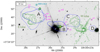 |
Fig. 1. Image of the FRII radio galaxy J103025+052430. In the background, we show the Hubble Space Telescope F160W-filter image (D’Amato et al. 2020). Radio JVLA contours (starting from 3σ) at 1400 MHz with 1.5 × 1.2 arcsec beam (D’Amato et al. 2022) are overlaid in green. The X-ray Chandra diffuse emission above 2.5σ in the soft band (0.5–2 keV) and hard band (2–7 keV) is shown with dashed and solid blue contours, respectively (Nanni et al. 2018; Gilli et al. 2019). Black letters A, B, C, and D mark the main X-ray components as defined in Gilli et al. (2019). Magenta circles mark the MUSE (m1–m5, Gilli et al. 2019) and ALMA (a1–a3, D’Amato et al. 2020) galaxies, which are part of the protocluster at z = 1.7 presented in Gilli et al. (2019). The SDSSJ1030+0524 quasar at z = 6.3 is marked with a cyan circle. The FRII radio galaxy host is marked with a yellow cross. Two galaxy members of the protocluster are located outside the displayed field of view: m6, located at ∼25 arcsec north of m2, and one source detected by LUCI, located at ∼1.5 arcmin south-east of the FRII radio galaxy host. |
The SDSSJ1030+0524 quasar field is very well studied based on the rich multi-wavelength observational campaign performed by our group. Results and data products can be found on the project webpage1. This also allows for a detailed investigation of the FRII. In particular, Nanni et al. (2018) detected diffuse extended X-ray emission using Chandra observations in the band 0.5 − 7 keV, mostly coinciding with its eastern lobe and central nucleus (see the blue and red contours in Fig. 1).
Later, using spectroscopic data collected with the Multi Unit Spectroscopic Explorer (MUSE) at the Very Large Telescope (VLT) and the Large Binocular Telescope (LBT) with the LBT Utility Camera in the Infrared (LUCI), Gilli et al. (2019) measured the redshift of the FRII galaxy and identified a galaxy overdensity that is composed of seven star-forming (star formation rate, SFR ∼ 8 − 60 M⊙ yr−1) galaxies around it (five of them are visible in Fig. 1 and are labelled m1–m5). Based on Atacama Large (sub-)Millimeter Array (ALMA) observations, three more gas-rich members of the system were later identified by D’Amato et al. (2020), with star formation rates in the range SFR ∼ 5 − 100 M⊙ yr−1 (labelled a1–a3 in Fig. 1).
The same FRII host is a highly star-forming galaxy with SFR 570 M⊙ yr−1 based on galaxy spectral energy distribution fitting (D’Amato et al. 2021). All member galaxies are distributed within a projected distance of 1.15 Mpc from the FRII host and span a redshift range of Δz = 0.012. The system is likely still not virialised, and based on the overdensity volume probed, it has a total mass of ≥3 × 10¹³ M⊙ (Gilli et al. 2019; D’Amato et al. 2020). Likely, it represents the early assembly phase of what will become a massive galaxy cluster (Msys > 1014 M⊙) in the z = 0 universe (D’Amato et al. 2020). In this view, it is also likely that the FRII host will evolve into the brightest cluster galaxy (BCG).
In the optical band and based on the NII/Hα ratio and narrow width of Hα, the FRII host is classified as a classical type 2 AGN (Gilli et al. 2019). The nuclear X-ray emission is also consistent with a heavily obscured (Compton thick) AGN, with a derived column density of NH, X ∼ 1024 cm−2 (Gilli et al. 2019). Its bolometric luminosity equal to Lbol = 4 × 1045 erg s−1 (as derived from the absorption-corrected X-ray luminosity equal to L2 − 10 keV = 1.3 × 1044 erg s, assuming a correction factor of 30 following Marconi et al. 2004), further suggests a classification as a quasar. Recent ALMA observations by D’Amato et al. (2020) showed that the FRII host is surrounded by an extended (≈20 kpc) and massive (MH2 = 2 × 10¹¹ M⊙) molecular gas reservoir, which may significantly contribute to the observed X-ray column density.
Using the Chandra observations presented by Nanni et al. (2018), which are the deepest so far for a distant FRII within a galaxy overdensity (480 ks), Gilli et al. (2019) suggested that the observed extended X-ray emission is likely due to a combination of non-thermal emission produced by IC scattering between the photons of the cosmic microwave background (CMB) and the relativistic electrons in the radio lobe, and thermal emission produced by an expanding bubble of gas that is shock-heated by the FRII jet.
Interestingly, four out of the six MUSE galaxies in the overdensity are distributed in an arc-like shape right at the edge of the diffuse X-ray emission around the eastern lobe of the FRII (see galaxies m1–m4 in Fig. 1). The measured specific star formation rates (sSFR) in these galaxies are higher by a factor from two to five than those measured in the other protocluster members and those of typical main-sequence galaxies of equal stellar mass and redshift (Gilli et al. 2019). This striking spatial coincidence and enhanced sSFR were interpreted as unique evidence of positive AGN feedback on multiple galaxies at high redshift, that is, star formation promoted by the expanding lobes, making it a unique object.
3. Data
3.1. LOFAR observations at 144 MHz
The target was observed with the LOFAR high-band antennas in the frequency range 120–168 MHz for a total observing time of 16 hours (see Table 1 for the observation setup). To obtain the best possible uv-coverage given the low declination of the target, the total observing time was split into four-hour observing blocks. The observation setup was created following the standard LOFAR Two-meter Sky Survey (LoTSS; Shimwell et al. 2019) strategy. Both Dutch and international stations were included in the observations, but the latter were not analysed here and will be presented in a future work. All four polarisations were recorded (XX, XY, YX, and YY), the correlator time was set to 1s, and the frequency resolution to 12.2 kHz. 3C 295 was observed for 10 min at the beginning of each observing run and used as primary calibrator.
LOFAR observation details.
Before being stored in the LOFAR long-term archive, the data were pre-processed using the observatory pipeline (Heald et al. 2010). This performed automatic flagging of radio frequency interference using the AOFlagger (Offringa et al. 2012) and averaged the data by a factor of 4 in frequency.
Using the PreFactor pipeline2 as described by van Weeren et al. (2016) and Williams et al. (2016), direction-independent calibration was performed, which corrects for ionospheric Faraday rotation, offsets between XX and YY phases, and clock offsets (see de Gasperin et al. 2019). Ionospheric distortions and errors in the beam model were then corrected using the DDF pipeline3, which performs various direction-dependent self-calibration cycles (Tasse et al. 2021 and Shimwell et al. 2019) using the software kMS (Tasse 2014 and Smirnov & Tasse 2015) and the imager DDFacet (Tasse et al. 2018). The calibration in the direction of the target was further improved by applying the procedure presented in van Weeren et al. (2021). This consists of subtracting from the visibilities all sources outside a square region centred on the target (here with a side equal to 24 arcmin), and performing a final direction-independent self-calibration round.
The final image deconvolution was performed with WSClean (version 2.8, Offringa et al. 2014) using a Briggs weighting scheme with robust = −0.5 (which optimises spatial resolution and noise pattern), multiscale cleaning, and applying an inner uv-cut at 40kλ. The final image (presented in Fig. 2) was restored with a beam of 6 arcsec × 6 arcsec (51 kpc × 51 kpc) and has an rms of 0.14 mJy beam−1.
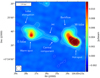 |
Fig. 2. LOFAR image of the radio galaxy J103025+052430 located at redshift z = 1.7 at a central frequency of 144 MHz. Labels mark the most significant morphological features in the source. The beam equal to 6 arcsec × 6 arcsec is shown in the bottom left corner. Contours are drawn at [−3, 3, 5, 10, 20, 50, 100, 200] ×σ, with σ = 0.14 mJy beam−1. |
A second image was also produced using the same aforementioned parameters, but excluding all baselines shorter than 1450λ. This cut corresponds to the shortest well-sampled baseline of the JVLA dataset at 1400 MHz (see Sect. 3.2) and is applied to recover the flux density on the same spatial scales at both frequencies and to perform a reliable spectral analysis (see Sect. 4.2).
The flux density scale of the final image was checked using the ten brightest sources in the field as reference. The flux densities of these sources from all publicly available surveys were used to extrapolate the expected flux densities at the frequencies of interest, and these were compared with the measured values. Following this procedure, we did not find any systematic offset in the flux density scale of the image within an uncertainty of 1σ. We assumed a conservative flux density scale calibration uncertainty equal to ΔSc = 20% following Shimwell et al. (2019, 2022). The flux density of the target is consistent with what was measured in the TIFR GMRT Sky Survey-Alternative Data Release (TGSS-ADR1; Intema et al. 2017) within the uncertainties.
3.2. Other data
In addition to the new LOFAR data at 144 MHz described in Sect. 3.1, we also used the JVLA dataset at 1400 MHz for the analysis in this work. This dataset was recently presented in D’Amato et al. (2022). This was obtained using A-array observations for a total observing time of ∼30 hours. For a full description of the data reduction procedures, we refer to (D’Amato et al. 2022). Here we re-imaged the calibrated data to match the properties of the LOFAR image and performed a resolved spectral analysis of the source in the frequency range 144-1400 MHz (see Sect. 4.2). To create the image, we used WSClean and the following parameters: a Briggs weighting scheme with robust = 0, a Gaussian taper of 5 arcsec, and a final restoring beam equal to 6 arcsec × 6 arcsec. The final image has an rms of 0.025 mJy beam−1. A flux density scale uncertainty equal to ΔSc = 5% was considered following Perley & Butler (2013).
The LOFAR and VLA images were spatially aligned to correct for spatial shifts introduced by the self-calibration. To do this, we used a bright point source in the field (RA = 10h30m16s and Dec = +05d23m03s). The source was fitted with a 2D Gaussian function, and its central pixel position was used as a reference for alignment. The procedure was carried out using the tasks imfit, imhead, and imregrid in the Common Astronomy Software Applications (CASA; McMullin et al. 2007) package. After this procedure, the images have a residual offset < 0.1 pixels, which is sufficiently accurate for our analysis.
Finally, we used the Chandra images in the energy range 0.5–7 keV, presented in Nanni et al. (2018) and Gilli et al. (2019). This allows for a comparison between the radio and X-ray emission of the system.
4. Analysis and results
4.1. Radio source properties
In Fig. 2 we present our new LOFAR image of the radio galaxy J103025+052430 at 144 MHz. The most relevant features are labelled in the figure. The source features two lobes and a central unresolved component, consistent with what has been observed at 1400 MHz (Petric et al. 2003; D’Amato et al. 2022). Moreover, a large-scale jet-like structure connecting the eastern lobe to the AGN nucleus is now clearly detected.
The western lobe shows a clear FRII-like structure, including a compact hotspot and a backflow bending towards the north-west. As already reported by D’Amato et al. (2022), the morphology of the eastern lobe is more unusual. It shows a surface brightness (SB) enhancement towards the southern edge that does not satisfy the classical definition of hotspot (i.e. SB ≥ 0.6 mJy arcsec−2 and an SB contrast with respect to the entire lobe ≥4; de Ruiter et al. 1990). It is therefore referred to as a warm spot. Moreover, in the north-east direction with respect to the warm spot, the eastern lobe shows a further elongation (see Fig. 2). Both the ratio between the jet and its counterjet and the polarisation analysis of the source suggest that the jet terminates in the warm spot (D’Amato et al. 2021; D’Amato et al. 2022), as detailed below. The polarisation image of the source shows two patches of emission in correspondence to the warm spot, similar to what is usually observed in the hotspots of FRII radio galaxies and suggesting that in this region, the jet impacts the surrounding medium and becomes compressed. Moreover, the magnetic field orientation experiences a 90-degree rotation moving from the warm-spot peak towards the centre of the lobe to the north, which might be indicative of the jets bending northwards after impacting the ICM. Furthermore, the radio galaxy inclination angle estimated from the jet versus counter-jet base flux density ratio (Gilli et al. 2019; D’Amato et al. 2022) agrees better with that estimated from the jet and counter-jet length ratio when the jet is assumed to end at the warm spot rather than at the end of the northern elongated region.
The origin of the complex morphology of the eastern lobe is unclear, but is not unusual in giant radio galaxies (e.g., Bruni et al. 2020; Cantwell et al. 2020; Carilli et al. 2022). It could be related to the jet being precessing (Donohoe & Smith 2016; Horton et al. 2020), being bent with respect to the observer line of sight (Harwood et al. 2020), or to the jet flow being deviated by a patchy external environment. The latter option would be particularly consistent with an unhomogeneous ambient medium, as expected in a protocluster environment, and could further justify the asymmetry with the western lobe-core axis (Pirya et al. 2012; Cantwell et al. 2020).
Overall, based on its morphology, the radio galaxy could be classified as a hybrid morphology radio source (Hymor; Gopal-Krishna & Wiita 2000; Harwood et al. 2020). This is a rare class of radio galaxies in which a different FRI/FRII morphology is observed for each of the two lobes.
The central component of the radio galaxy at 144 MHz is unresolved, implying an upper limit to its physical extension of ∼50 kpc. Observations at 1400 MHz with higher resolution (Fig. 1) show that this region includes both the actual nuclear emission and the base of the eastern jet.
When the 3σ contours are used as a reference, the total projected extension of the source in the LOFAR image is ∼90 arcsec, which corresponds to ∼750 kpc. This is consistent with previous estimates made using the 1.4 GHz image (D’Amato et al. 2022). This places the source within the giant radio galaxy population (GRG; Kuźmicz & Jamrozy 2021). Based on considerations of the jet-counterjet flux density ratio and length ratio, D’Amato et al. (2022) computed that the source inclination with respect to the line of sight is equal to ∼80 deg, with the eastern jet approaching the observer. By accounting for the source inclination, we obtain that the intrinsic extension of the source must be 750/cos θ ≈ 800 kpc.
We stress that while recent observational efforts have significantly increased the detection number of giant radio galaxies and giant radio quasars (GRQs; e.g., Kuźmicz et al. 2018; Dabhade et al. 2020a,b; Bruni et al. 2020; Kuźmicz & Jamrozy 2021; Delhaize et al. 2021; Andernach et al. 2021; Simonte et al. 2022; Mahato et al. 2022, Oei et al. 2023), the number of giant radio sources identified at redshift z > 1.5 remains limited to date (10 out of 239 in the sample of Dabhade et al. 2020b; 33 out of 272 in the sample of Kuźmicz & Jamrozy 2021; 3 out of 178 in the sample of Andernach et al. 2021; and 7 out of 74 in the sample of Simonte et al. 2022), possibly due to observational limits.
The total flux density of J103025+052430 at 144 MHz and 1400 MHz, as well as the flux densities of the individual morphological components, is listed in Table 2, together with the respective luminosities. These were measured from the 6 arcsec resolution maps at both frequencies for consistency and using the black regions shown in the right panel of Fig. 3, which were drawn following the 3σ contours at 144 MHz. The total uncertainty (ΔS) on the flux densities (S) was computed by combining the flux density scale calibration uncertainty (ΔSc) and the image rms noise (σ) in quadrature, multiplied by the flux density integration area in beam units (Aint),
 (1)
(1)
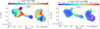 |
Fig. 3. Radio spectral index map of J103025+052430 in the range 144–1400 MHz with 6 arcsec resolution (left panel) and respective spectral index uncertainty map (right panel). The spectral index values across the radio galaxy vary in the range [0.46–1.78], but the colour scale has been compressed for visualisation purposes. Only pixels above 3σ in both images are used. The beam size is shown in the bottom left corner. Contours in the left panel represent the 144-MHz emission as shown in Fig. 2 (left panel). White contours in the right panel represent the JVLA 1400-MHz emission at 1 arcsec resolution presented in D’Amato et al. (2022). with levels equal to [−3, 3,5, 10, 20, 50, 100, 200]×σ, with σ = 0.004 mJy beam−1. Black regions in the right panel represent the regions we used to measure the flux densities listed in Table 2. The spectral index distribution of the source is overall consistent with what is typically observed in FRII radio galaxies. The compact source at RA = 10h30′27″ Dec = 5d24m50s is an unrelated source. |
Source properties as measured in the 6 arcsec images.
The integrated spectral indices and k-corrected radio powers are also presented in Table 2. The spectral index uncertainties were estimated with the following formula based on the propagation of error:
 (2)
(2)
where S144 MHz and S1400 MHz are the flux density values at the respective frequencies in MHz, and ΔS144 MHz and ΔS1400 MHz are their corresponding uncertainties.
With a power of P144 MHz ∼ 3 × 1027 W Hz−1, J103025+052430 appears to be among the 30 most powerful giant radio sources (with P144 MHz > 1027 W Hz−1) in the sample of 239 GRGs and GRQs (optically selected; see Duncan et al. 2019) extracted by Dabhade et al. (2020b) from LoTSS.
The integrated spectral index of the source is  and lies well within the observed integrated spectral index distribution derived for the aforementioned sample: the full range is equal to
 ![Mathematical equation: $ \alpha_{144\,\rm MHz}^{1400\,\rm MHz}=[0.4,1.5] $](/articles/aa/full_html/2023/04/aa45247-22/aa45247-22-eq5.gif) , and the median values are equal to
, and the median values are equal to  and
and  for GRGs and GRQs, respectively. These values are not different from those observed in active radio galaxies of smaller size (e.g., Parma et al. 1999; Mullin et al. 2008), thus confirming that despite the large size, giant radio sources are not remnant (inactive) sources, and that their integrated spectral index is dominated by freshly accelerated particles. The measured spectral index of J103025+052430 is also consistent with the values observed for the ten sources at the highest redshift (1.5 < z < 2.3) in the same sample.
4.2. Radio spectral index distribution
To investigate the spectral index variations across the source, we created the spectral index map presented in the left panel of Fig. 3 by combining the matched images at 144 MHz and 1400 MHz described in Sect. 3. Only pixels with surface brightness values above 3σ in both maps were included. The spectral index uncertainty map is shown in the right panel of Fig. 3. It was obtained using Eq. (2), where S144 and S1400 this time correspond to the surface brightness values of each pixel at the respective frequencies, and ΔS is computed with Eq. (1) using Aint = 1.
The spectral index values across the source vary in the range [0.46-1.78]. Overall, the observed spectral index distribution supports the FRII classification made previously based on the source morphology alone. In the lobes of these sources, the flattest spectral index values are observed at the lobe edges, where the actual particle acceleration occurs. The compact component at the centre shows a flatter spectral index with a mean value of  , consistent with being produced by a superposition of nuclear activity and the base of the jet (e.g., Orrù et al. 2010; Harwood et al. 2016).
In the eastern lobe, the mean spectral index is  . Interestingly, the spectral index map (Fig. 3) shows that the flattest spectral index is not observed exactly in coincidence with the warm spot, which was previously claimed to represent the jet termination region. Instead, the region with the flatter spectral index (with values down to
  ) is located along the entire edge of the eastern lobe. No special spectral index trend is instead observed in correspondence to the polarisation enhancement and magnetic field alignment reported by D’Amato et al. (2021) at the northern edge of the lobe, which were suggested to be consistent with the lobe being compressed. A flatter spectral index at this location would have been expected in this case.
The spectral index in the western hotspot has a minimum value of  , consistent with what is observed in other similar sources (e.g., Vaddi et al. 2019). As shown in Fig. 3, away from the hotspot and across the backflow northwards, the spectral index steepens up to values of
  , as expected for ageing plasma (Pacholczyk 1970). Interestingly, towards the north-eastern edge of the western lobe, there is a tentative indication that the spectral index flattens again.
To investigate this trend further, we created a spectral index profile using five square regions distributed along the lobe, with sides equal to 6 arcsec (∼50 kpc), corresponding to the beam size (see Fig. 4, left panel). We note that the result is the same when we slightly change the orientation of the boxes. The profile shows that the spectral index reaches a maximum value of  in region 4 and then decreases to a value of
  in region 5.
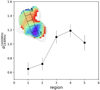 |
Fig. 4. Spectral index profile in the frequency range 144–1400 MHz across the western lobe of J103025+052430. The regions we used to extract the spectral profile are shown as black boxes overlaid on the lobe in the top left corner and have sizes equal to the beam dimension (6 arcsec = 50 kpc). In the outermost region of the backflow, the spectral index shows a tentative flattening, as discussed in Sect. 4.2. |
This trend might be suggesting that the backflow is compressed by the interaction with the surrounding medium. Compression indeed enhances the number density of relativistic electrons and of the magnetic field. This translates into an increase in brightness, as well as into a shift of the spectrum towards higher frequencies. This happens because the bulk of the synchrotron radiation released by each particle of energy E = γmec2 is emitted at the critical frequency νc,
 (3)
(3)
where γ is the Lorentz factor, me is the electron mass, c is the speed of light, e is the electron charge, and B is the magnetic field. When the magnetic field increases in the compressed plasma, the critical frequency of each particle will also increase, causing an overall shift of the entire spectrum towards higher frequencies.
As shown in Fig. 5, the region in which the flattening is observed coincides with the diffuse X-ray emission labelled component C (see Sect. 4.3.2). The measured trend of the radio spectral index might indicate that at this location, the radio-emitting plasma indeed interacts with and compresses the external thermal medium, enhancing its X-ray brightness. Unfortunately, due to the low radio brightness of the backflow emission at 1.4 GHz, D’Amato et al. (2021) were unable to detect any polarisation signal, which could have helped to investigate the compression scenario. Future multi-frequency radio observations at higher resolution are needed to confirm this trend.
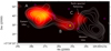 |
Fig. 5. Diffuse X-ray emission (components A, B, and C) as seen by Chandra in the full 0.5–7 keV band with LOFAR 144-MHz contours overlaid in white (same as Fig. 2). The protocluster galaxy members as reported in Fig. 1 are marked with magenta circles, and the radio galaxy host is marked with a yellow cross. |
Using the broadband radio astronomy tool software package (BRATS; Harwood et al. 2013) we obtained that it takes 8 Myr for the plasma to reach a spectral index equal to  , which is the steepest spectral index value observed in the radio galaxy. For this first-order age derivation, we used a Jaffe-Perola radiative model (Jaffe & Perola 1973) and assumed an injection index of αinj = 0.6 (assumed to be the same as the spectral index observed in the hotspot, where particle acceleration occurs) and a magnetic field equal to 1.3–2 μG (see Sect. 4.3.1 for a full discussion of the magnetic field derivation). We note, however, that this estimate is almost independent of the assumed magnetic field as the particle energy losses at this redshift are dominated by IC losses (Hodges-Kluck et al. 2021), which are a factor ∼20 higher than those for synchrotron Compton (BCMB = 3.25 ⋅ (1 + z)2).
4.3. X-ray diffuse emission
As shown in Fig. 1 and discussed in Nanni et al. (2018) and Gilli et al. (2019), the Chandra image of the system reveals several components of emission in both the soft (0.5–2 keV) and hard (2–7 keV) bands. In particular, component A approximately shows an equal amount of soft and hard X-ray emission, and was suggested to be mostly ascribed to gas that is shock-heated by the passage of the eastern jet, possibly combined with a contribution from CMB IC scattering. Component B, mostly visible in the hard band, is consistent with a non-thermal origin related to the jet or core of the FRII radio galaxy. Component C is instead detected in the soft band and is consistent with a thermal origin. Finally, beyond the western hotspot, we tentatively detect (∼2σ) a further spot of soft X-ray emission marked D, which is also consistent with a thermal origin. In the light of the new radio data, we discuss these results further.
4.3.1. Component A
Gilli et al. (2019) investigated the origin of the X-ray emission observed in component A. The X-ray spectrum was fitted with both a purely thermal model and a power-law model, which returned a gas temperature equal to > 5 keV and a photon index equal to  , respectively. Because of the low number counts, the fit statistics was unfortunately found to be inconclusive for either of the two fits. However, when the observed X-ray emission is compared with the available radio data, a thermal origin interpretation was preferred over non-thermal origin.
The new LOFAR and JVLA images show now much more clearly that the radio emission of the eastern lobe entirely overlaps with component A and that component B overlaps with the core and the well-visible eastern jet (see Fig. 5). The confirmation of this spatial coincidence reinforces the argument that the radio and X-ray emission are physically connected. Moreover, the spectral index in the hotspot of the western lobe of the radio galaxy is equal to αinj = 0.6 ± 0.1, suggesting that the particle energy injection index in the radio galaxy is p ∼ 2.2 (p = 2α + 1), which is consistent with the power-law photon index  (with Γ = α + 1) derived from the X-ray spectral analysis in the IC scenario (Gilli et al. 2019).
Using our new estimates for the source volume and spectral index as well as new considerations on the magnetic field based on results from the literature, we revised the calculations presented by Gilli et al. (2019) as shown below. We estimated the magnetic field Bme of the eastern lobe using the minimum-energy assumption following Eq. (2) in Miley (1980) and applying the revision proposed by Brunetti et al. (1997) to account for the contribution from lower-energy electrons, which might be missed by integrating over frequency. The equations are reported below:
![Mathematical equation: $$ \begin{aligned}&B_{\mathrm{me} }=5.69 \times 10^{-5}\left[\frac{(1+ k)}{\eta }(1+z)^{3+\alpha }\right. \frac{1}{\theta _{x} \theta _{{ y}} \,l \sin ^{3 / 2} \phi } \nonumber \\&\qquad \quad \left.\times \frac{S_{\rm obs}}{\nu _{\rm obs}^{-\alpha }} \frac{\nu _{2}^{ 0.5-\alpha }-\nu _{1}^{ 0.5-\alpha }}{0.5-\alpha }\right]^{2 / 7} \ \mathrm{Gauss}, \end{aligned} $$](/articles/aa/full_html/2023/04/aa45247-22/aa45247-22-eq19.gif) (4)
(4)
 (5)
(5)
where the symbols have the following meaning: θx, θy are the angular dimensions of the radio source in arcsec along the x- and y-axis; k is the ratio proton-to-electron ratio; η is the filling factor of the emitting region; l is the path length through the source in kiloparsec; Sobs is the radio flux density (in Jy) of the region at the observed frequency νobs (in GHz); α is the spectral index; ν1, ν2 are the lower and upper cut-off frequencies presumed for the radio spectrum (in GHz); ϕ is angle between the magnetic field and the line of sight; p = 2α + 1 is the particle energy index distribution; γmin is the minimum Lorentz factor of the particle distribution.
We assumed k = 1, η = 1, ϕ = 90°, ν1 = 0.01 GHz, and ν2 = 100 GHz following Gilli et al. (2019). For the flux density, we used the value reported in Table 2 equal to Sobs = 35 mJy at νobs = 144 MHz. For the size, we used θx = 22 arcsec and θy = 34 arcsec, as measured from the LOFAR image using the 3σ contours as a reference, and we assumed that the radial direction l is equal to the transverse direction θx = l = 190 kpc. Based on the LOFAR-JVLA spectral index map now available (see Fig. 3), we set the spectral index to α = 0.6 (and thus p = 2.2), which is the flattest value observed in the western hotspot and reasonably corresponds to the injection index value of the plasma within the lobes. D(γ) = 1.01 and γmin = 20 were set following Brunetti et al. (1997). According to this, the revised equipartition magnetic field value is Bme, rev = 4 μG.
We note, however, that in recent years, an increasing number of studies in the literature (e.g., Croston et al. 2005; Kataoka & Stawarz 2005; Migliori et al. 2007; Isobe et al. 2011; Ineson et al. 2017; Turner et al. 2018) have shown that magnetic fields in FRII radio galaxies are typically a factor of 2–3 lower than the values derived based on minimum-energy arguments. If this were also the case for J103025+052430, we would then expect that the actual magnetic field value is in the range Bfinal = 1.3–2 μG.
Assuming these last values, we can then compute the X-ray emission expected from IC scattering of CMB photons by the relativistic electrons (IC-CMB) in the eastern lobe using Eq. (11) of Harris & Grindlay (1979),
 (6)
(6)
Here SX and Sr (see Table 1) are the X-ray and radio flux densities in cgs units, and B is the magnetic field in Gauss. C(α) and G(α) are slowly varying functions of α (see e.g., Harris & Grindlay 1979; Pacholczyk 1970): We assumed G(α) = 0.521 (it goes from 0.521 for α = 0.6, to 0.5 for α = 1.0) and C(α) = 1.15 × 1031, which is good within 17% for 0.5 < α < 2.0.
By posing B = Bfinal and assuming that the X-ray spectrum is a power law with spectral index α = 0.6, that is, equal to the radio injection index and also consistent within the uncertainties with what we measured with Chandra for component A, we derived an X-ray flux in the 0.5–7 keV band of f0.5−7 keV ∼ (1.6 − 2.9) × 10−15 erg cm−2 s−1.
This corresponds to a fraction of ∼45%−80% of the 0.5–7 keV flux measured from the Chandra image for component A (f0.5−7 keV ≃ 3.7 × 10⁻¹⁵ erg cm−2 s−1; Gilli et al. 2019), suggesting that a significant fraction of the observed X-ray emission likely originated by IC scattering with the CMB. This is further supported by the clear spatial coincidence of the X-ray component A and the eastern lobe, as seen now by our new LOFAR observations.
We note that the synchrotron-emitting particles that upscatter CMB photons (νCMB) to higher frequencies (νX) are expected to have Lorentz factors γ equal to (see e.g., Blundell et al. 2006)
 (7)
(7)
By assuming that the photons from the peak of the CMB distribution are IC upscattered by the radio-emitting electrons in the lobes or jets, the Lorentz factor of the particles that cause the emission observed at 1 keV is γ ∼ 800. For magnetic fields in the range Bfinal = 1.3–2 μG, this corresponds to particles emitting at about a few dozen megahertz, which is below the observed radio range. The use of a spectral index equal to α = 0.6, closer to injection, for Eq. (6) is then the best approximation we can make for the energy distribution of the upscattered particles.
4.3.2. Component C
As already mentioned in Sect. 4.2, the X-ray component C overlaps with the backflow of the western radio lobe and might represent a signature of the interaction between lobe and ICM. This spot of emission extends for about 20 arcsec and is detected in the full and soft band (with a significance of S/N ∼ 2.4 and 3.4, respectively) but not in the hard band. Despite the overall low-detection significance, we are confident that component C is real because it is also visible in the XMM-Newton observation of the field presented by Nanni et al. (2018). The X-ray spectrum of component C is well fitted by a thermal model with T ≃ 1 keV, while a power-law fits returns implausibly high photon indices equal to Γ ∼ 4–5, which supports a thermal origin (Gilli et al. 2019).
We further investigated the pressure balance of this component with respect to its surrounding environment. By fixing the metallicity of the hot emitting plasma to 0.3× solar (e.g., Balestra et al. 2007), its temperature was estimated to be  keV (Gilli et al. 2019). Assuming that the plasma is distributed within a sphere of 85 kpc radius (i.e. 10 arcsec projected radius, as measured from the Chandra image), with the measured source temperature and normalisation of the best-fit plasma model (APEC within XSPEC), we derived a particle density within component C of ne = 2.3(±0.7)×10−2 cm−3. For reference, this is about six times higher than what was derived for component A by Gilli et al. (2019), assuming that all its X-ray emission was of thermal origin. The measured density in the hot gas bubble C translates into a thermal pressure of P ∼ nekT = 2.3 × 10⁻¹¹ erg cm−3.
We note that, even assuming a mild metallicity evolution with redshift, the assumed value of 0.3× solar is reasonable for the redshift of the source equal to z = 1.7 (see e.g., Vogelsberger et al. 2018; Flores et al. 2021). Our result for the bubble pressure balance also remains unchanged when a more significant decrease in metals with redshift is considered. By assuming a more conservative value of 0.1× solar, we computed that T would decrease by only ∼7% and the electron density would increase by ∼30%, which is well within the measurement errors.
It is then interesting to compare whether this bubble is in pressure equilibrium with the ambient medium around it. Gilli et al. (2019) assumed that most of the protocluster medium is in the form of atomic gas with a temperature T < 105 K and a column density NH ∼ 1019 − 20 cm−2 because a similar medium is observed in other z ∼ 2 protoclusters (e.g., Cucciati et al. 2014; Hennawi et al. 2015). It is easy to show that the pressure in bubble C would largely exceed the pressure of such a medium.
However, the cool medium pressure estimated in Gilli et al. (2019) is likely a lower limit to the total pressure of the ambient medium, which could be dominated by that of a tenuous, warm-hot medium with T = 105 − 7 K that is notoriously difficult to reveal (Nicastro et al. 2018). Under the conservative hypothesis that this medium pervades the protocluster and contains most baryons, we derived its particle density as nICM = MICM/(mpV), where V is the protocluster volume, mp is the proton mass, and MICM is the enclosed ICM mass. The latter can be estimated as MICM = 0.17 × MDM, where MDM is the total dark matter mass in the protocluster, and 0.17 is the universal baryon fraction (Spergel et al. 2007).
D’Amato et al. (2020) measured the dark matter mass enclosed within a volume of 3.9 Mpc3 around the FRII radio galaxy. This volume corresponds to the sky area covered by the ALMA observations presented in that paper (∼2 sq. arcmin) times the radial separation given by the maximum redshift interval between member galaxies (Δz = 0.012). By means of both the velocity dispersion of member galaxies and the measured overdensity level, the authors estimated an enclosed dark matter mass of MDM ∼ 6 × 10¹³ M⊙.
With the above numbers in hand, we derived a particle density for the ambient medium of nAM = 1.1 × 10⁻⁴ cm−3, and in turn a ratio of the thermal pressure of bubble C and that of the surrounding ambient medium of PbubC/PAM = 1.6 × 10⁹ TICM(K). This implies that even assuming an extremely hot ambient medium with a temperature of 107 K, the bubble of gas C is still highly overpressurised and therefore expands rapidly. In this process, it will likely release its energy, contributing to the overall heating of the surrounding intracluster medium.
The timescale on which bubble C is expected to cool owing to bremsstrahlung emission is (Mo et al. 2010; Costa et al. 2014; Gilli et al. 2017)
 (8)
(8)
where T and ne are the gas temperature in K and the gas density in cm−3. For ne = 0.023 cm−3 and kT = 0.63 keV (T = 7.3 × 10¹⁰ K) as measured in bubble C, tcool ∼ 0.9 Gyr. The bubble cooling time is then much longer than the estimated AGN lifetime (∼70 Myr; Gilli et al. 2019), and the bubble has then likely expanded adiabatically thus far. However, tcool is shorter than the ∼10 Gyr it will take for the structure to evolve into a massive > 1 × 10¹⁴ Msun cluster by z = 0 (D’Amato et al. 2020). By then, the bubble will have radiated away all its energy (Eth = 3neVkT ∼ 5 × 1060 erg), part of which may couple with the ambient medium and contribute to the overall ICM heating together with PdV work and mixing (e.g., Bourne et al. 2019).
5. Discussion and conclusions
With its broad multi-band coverage, the giant radio galaxy J103025+052430 at z = 1.7 represents an exceptional laboratory in which we can test how AGN jet feedback influences the growth of galaxies at high redshift and study the evolution of the ICM before virialisation. In this paper, we have reported new LOFAR observations at 144 MHz of the system, which we used in combination with already published VLA observations at 1.4 GHz (D’Amato et al. 2021; D’Amato et al. 2022) and 0.5–7 keV Chandra observations (Gilli et al. 2019).
The large angular (and thus physical) size of the source enabled us to perform a resolved radio spectral index analysis in the frequency range 144–1400 MHz (see Sect. 4.2), which is a very unique opportunity for a source at such a high redshift. The oldest observable radio-emitting particles have ages of ∼8 Myr, suggesting that the jets have been active for at least this time.
The observed spectral index distribution is overall consistent with expectations for FRII radio galaxies, but it also shows an unexpected pattern: there is a hint of spectral flattening at the edge of the backflow in the western lobe. In the backflow, particles are expected to lose their energy with time and to show increasingly steeper spectral index values away from the site of acceleration (the hotspot). The detection of this flattening can thus only be explained with a scenario in which particles at the edge of the backflow interact with the external medium and are re-energised.
Interestingly, the end of the backflow happens to be co-spatial (at least in projection) with the X-ray component C, which was shown to have a thermal origin by Gilli et al. (2019). The heat source for component C is unclear. One natural hypothesis would be that the X-ray emitting gas is heated and compressed by the passage of the jet and in particular by the expanding radio-lobe backflow. It is important to stress that because it is overpressurised with respect to the ambient medium (see Sect. 4.3.2), bubble C will likely expand and deposit its energy in the surrounding gas on a timescale of ∼0.9 Gyr, thus contributing to the overall ICM heating well before virialisation.
While much less significant than component C, component D, located just beyond the position of the western hotspot (see Fig. 1) and also consistent with a thermal origin, could also represent a region in which the ambient medium is compressed by the expanding jet. If this is the case, it might be wondered why, given its position close to the hotspot (where the jet pressure on the ICM is strongest), its X-ray luminosity is lower than that of component C. One simple possibility is that because the X-ray luminosity expands as the density squared, a density difference by only a factor of 1.4 between the two components could justify the observed luminosity difference. This density difference is not implausible considering that the system is likely still not virialised and its baryon content is likely inhomogeneous.
For the eastern lobe, as already mentioned in Sect. 4.3.1, Gilli et al. (2019) proposed that the X-ray emission in component A was the result of gas that was shock-heated by the jet or lobe. Based on our new LOFAR and JVLA observations, we revised the estimate of the CMB IC scattering contribution to the X-ray emission co-spatial with the eastern lobe and found that it can account for most (∼45%–80%) of the total 0.5–7 keV measured flux. This appears to reduce the role of the shock scenario previously proposed, but according to our numbers, it is not excluded that a non-negligible fraction of the total observed emission is still of thermal origin related to the ICM.
Observations of CMB-IC emission associated with (giant) radio galaxies at z > 1 is not unusual (e.g., Overzier et al. 2005; Erlund et al. 2006, 2008; Johnson et al. 2007; Laskar et al. 2010; Tamhane et al. 2015; Hodges-Kluck et al. 2021; Carilli et al. 2022; Tozzi et al. 2022). In a few cases, claims have also been made for the presence of IC ghosts, that is, IC emission associated with old lobes of radio galaxies that has become invisible at radio frequencies due to the quick energy losses (Fabian et al. 2003, 2009; Mocz et al. 2011). Detecting the thermal emission from the ICM is instead much more challenging, especially on scales of hundreds of kiloparsec. In the case of J103025+052430, disentangling its contribution from the IC contribution to the total observed X-ray emission would require high-resolution high-sensitivity observations, like for example in the case of the Spiderweb field (Carilli et al. 2022; Tozzi et al. 2022).
We note that even if the origin of the X-ray emission in component A were entirely non-thermal, the conclusions about feedback drawn by Gilli et al. (2019) do still hold because star formation in the galaxies m1–m4 (see Fig. 1) may be promoted by the non-thermal pressure of the expanding lobe and the shocks associated with them.
Overall, the protocluster J103025+052430 with its central radio galaxy is one of the best-characterised systems and one of the nicest examples of jet AGN feedback on scales of hundreds of kiloparsec at z > 1.5. Based on the estimated overdensity volume, the mass of the system is ≥3 × 10¹³ M⊙ (Gilli et al. 2019; D’Amato et al. 2020), which meas that it will likely evolve into a galaxy cluster with Msys > 1014 M⊙ at z = 0 (D’Amato et al. 2020). It thus provides us with a unique opportunity to look back in the history of nearby rich clusters, such as the famous clusters Perseus and Abell 2256, and it surely deserves further investigation.
Future observations in both the radio and X-ray band are now urgently needed to confirm the current scenario. On the one hand, deeper X-ray observations would allow us to detect the diffuse emission at higher S/N, investigating the morphology of the brightest patches (e.g., components A and C, including any possible sharp drop in brightness), confirming the presence of the faintest patches (component D), and possibly discover new, even fainter patches. Moreover, they would enable a more robust spectral analysis that is able to distinguish between the thermal or non-thermal nature of component A, and place tighter constraints on the temperature of components C and D. Currently, the only instrument that may provide this improvement is Chandra, as it features the sharp resolution on the scale of arcseconds and has the sensitivity required to detect faint diffuse X-rays after removal of point source contaminants. Nonetheless, this requires significant time investments (≳Msec), as the effective area of Chandra is relatively small (∼600 cm2 at 1 keV in the first cycles). In the future, next generation X-ray missions such as the Survey and Time-domain Astrophysical Research eXplorer (STAR-X4), a medium explorer mission selected by NASA for phase A study, and the Advanced X-ray Imaging Satellite (AXIS; Mushotzky et al. 2019; Marchesi et al. 2020), a probe-class mission proposed to NASA, will have the sufficient 1–2 arcsec angular resolution and the large effective area (∼3 − 10× that of Chandra) required to investigate this and other high-z protoclusters with moderately deep exposures (tens to hundreds of kiloseconds), allowing population studies, and hence opening a new discovery space for structure formation.
From the radio point of view, new observations at complementary frequencies that have a resolution higher by a factor of a few are needed to produce more detailed spectral index maps and confirm the compression scenario proposed based on the observed spectral index trend in the western lobe. LOFAR observations at 55∼144 MHz with the international stations reaching a resolution ≲1 arcsec and observations with the upgraded Giant Meterwave Radio Telescope (GMRT; Gupta et al. 2017) at 400–700 MHz with a resolution of a few arcseconds are planned to pursue this goal. Faraday rotation and (de-)polarisation analysis at frequencies ≳1.4 GHz could also provide interesting information on the magneto-ionic properties of the ICM surrounding the radio galaxy and their interplay (e.g., Carilli & Taylor 2002; Guidetti et al. 2011; Anderson et al. 2022), and ALMA/ACA observations could be used to investigate the presence of any Sunyaev-Zeldovich effect signal and thus to more robustly constrain the pressure of component C (e.g., Abdulla et al. 2019; Di Mascolo et al. 2021).
Acknowledgments
M. Brienza would like to thank Giulia Migliori for the useful discussions. MB acknowledges financial support from the Italian L’Oreal UNESCO “For Women in Science” program, from the ERC-Stg “DRANOEL”, no. 714245 and from the ERC-Stg “MAGCOW”, no. 714196. MB and IP acknowledge support from INAF under the SKA/CTA PRIN “FORECaST”. IP acknowledges support from INAF under the PRIN MAIN STREAM “SAuROS” projects. We acknowledge support from the agreement ASI-INAF n. 2017-14-H.O and fr om the PRIN MIUR 2017PH3WAT “Blackout”. KI acknowledges support by the Spanish MCIN under grant PID2019-105510GB-C33/AEI/10.13039/501100011033. FV acknowledges the computing centre of INAF – Osservatorio Astrofisico di Catania, under the coordination of the WG-DATI of LOFAR-IT project, for the availability of computing resources and support. LOFAR, the Low Frequency Array designed and constructed by ASTRON, has facilities in several countries, which are owned by various parties (each with their own funding sources), and are collectively operated by the International LOFAR Telescope (ILT) foundation under a joint scientific policy. The ILT resources have benefited from the following recent major funding sources: CNRS-INSU, Observatoire de Paris and Université d’Orléans, France; BMBF, MIWF-NRW, MPG, Germany; Science Foundation Ireland (SFI), Department of Business, Enterprise and Innovation (DBEI), Ireland; NWO, The Netherlands; the Science and Technology Facilities Council, UK; Ministry of Science and Higher Education, Poland; The Istituto Nazionale di Astrofisica (INAF), Italy. Part of this work was carried out on the Dutch national e-infrastructure with the support of the SURF Cooperative through grant e-infra 160022 & 160152. The LOFAR software and dedicated reduction packages on https://github.com/apmechev/GRID_LRT were deployed on the e-infrastructure by the LOFAR e-infragrop, consisting of J. B. R. Oonk (ASTRON & Leiden Observatory), A. P. Mechev (Leiden Observatory) and T. Shimwell (ASTRON) with support from N. Danezi (SURFsara) and C. Schrijvers (SURFsara). The Jülich LOFAR Long Term Archive and the German LOFAR network are both coordinated and operated by the Jülich Supercomputing Centre (JSC), and computing resources on the supercomputer JUWELS at JSC were provided by the Gauss Centre for supercomputing e.V. (grant CHTB00) through the John von Neumann Institute for Computing (NIC). This research made use of the University of Hertfordshire high-performance computing facility and the LOFAR-UK computing facility located at the University of Hertfordshire and supported by STFC (ST/P000096/1), and of the Italian LOFAR IT computing infrastructure supported and operated by INAF, and by the Physics Department of Turin University (under an agreement with Consorzio Interuniversitario per la Fisica Spaziale) at the C3S Supercomputing Centre, Italy. This research made use of APLpy, an open-source plotting package for Python hosted at https://github.com/aplpy/.
References
- Abdulla, Z., Carlstrom, J. E., Mantz, A. B., et al. 2019, ApJ, 871, 195 [NASA ADS] [CrossRef] [Google Scholar]
- Andernach, H., Jiménez-Andrade, E. F., & Willis, A. G. 2021, Galaxies, 9, 99 [NASA ADS] [CrossRef] [Google Scholar]
- Anderson, C. S., Carilli, C. L., Tozzi, P., et al. 2022, ApJ, 937, 45 [NASA ADS] [CrossRef] [Google Scholar]
- Balestra, I., Tozzi, P., Ettori, S., et al. 2007, A&A, 462, 429 [NASA ADS] [CrossRef] [EDP Sciences] [Google Scholar]
- Best, P. N., Longair, M. S., & Rottgering, H. J. A. 1997, MNRAS, 286, 785 [NASA ADS] [CrossRef] [Google Scholar]
- Bicknell, G. V., Sutherland, R. S., van Breugel, W. J. M., et al. 2000, ApJ, 540, 678 [NASA ADS] [CrossRef] [Google Scholar]
- Blundell, K. M., Fabian, A. C., Crawford, C. S., Erlund, M. C., & Celotti, A. 2006, ApJ, 644, L13 [NASA ADS] [CrossRef] [Google Scholar]
- Bourne, M. A., Sijacki, D., & Puchwein, E. 2019, MNRAS, 490, 343 [NASA ADS] [CrossRef] [Google Scholar]
- Brunetti, G., Setti, G., & Comastri, A. 1997, A&A, 325, 898 [NASA ADS] [Google Scholar]
- Bruni, G., Panessa, F., Bassani, L., et al. 2020, MNRAS, 494, 902 [Google Scholar]
- Cantwell, T. M., Bray, J. D., Croston, J. H., et al. 2020, MNRAS, 495, 143 [Google Scholar]
- Capetti, A., Balmaverde, B., Tadhunter, C., et al. 2022, A&A, 657, A114 [NASA ADS] [CrossRef] [EDP Sciences] [Google Scholar]
- Carilli, C. L., & Taylor, G. B. 2002, ARA&A, 40, 319 [NASA ADS] [CrossRef] [Google Scholar]
- Carilli, C. L., Harris, D. E., Pentericci, L., et al. 2002, ApJ, 567, 781 [NASA ADS] [CrossRef] [Google Scholar]
- Carilli, C. L., Anderson, C. S., Tozzi, P., et al. 2022, ApJ, 928, 59 [NASA ADS] [CrossRef] [Google Scholar]
- Carniani, S., Marconi, A., Maiolino, R., et al. 2017, A&A, 605, A105 [NASA ADS] [CrossRef] [EDP Sciences] [Google Scholar]
- Chambers, K. C., Miley, G. K., & van Breugel, W. J. M. 1990, ApJ, 363, 21 [NASA ADS] [CrossRef] [Google Scholar]
- Chen, R.-R., Strom, R., & Peng, B. 2018, ApJ, 858, 83 [NASA ADS] [CrossRef] [Google Scholar]
- Chiaberge, M., Capetti, A., Macchetto, F. D., et al. 2010, ApJ, 710, L107 [NASA ADS] [CrossRef] [Google Scholar]
- Clark, N. E., Tadhunter, C. N., Morganti, R., et al. 1997, MNRAS, 286, 558 [NASA ADS] [CrossRef] [Google Scholar]
- Costa, T., Sijacki, D., & Haehnelt, M. G. 2014, MNRAS, 444, 2355 [Google Scholar]
- Croft, S., van Breugel, W., de Vries, W., et al. 2006, ApJ, 647, 1040 [NASA ADS] [CrossRef] [Google Scholar]
- Croston, J. H., Hardcastle, M. J., Harris, D. E., et al. 2005, ApJ, 626, 733 [NASA ADS] [CrossRef] [Google Scholar]
- Croton, D. J., Springel, V., White, S. D. M., et al. 2006, MNRAS, 365, 11 [Google Scholar]
- Cucciati, O., Zamorani, G., Lemaux, B. C., et al. 2014, A&A, 570, A16 [NASA ADS] [CrossRef] [EDP Sciences] [Google Scholar]
- Dabhade, P., Mahato, M., Bagchi, J., et al. 2020a, A&A, 642, A153 [NASA ADS] [CrossRef] [EDP Sciences] [Google Scholar]
- Dabhade, P., Röttgering, H. J. A., Bagchi, J., et al. 2020b, A&A, 635, A5 [NASA ADS] [CrossRef] [EDP Sciences] [Google Scholar]
- D’Amato, Q., Gilli, R., Prandoni, I., et al. 2020, A&A, 641, L6 [NASA ADS] [CrossRef] [EDP Sciences] [Google Scholar]
- D’Amato, Q., Prandoni, I., Brienza, M., et al. 2021, Galaxies, 9, 115 [CrossRef] [Google Scholar]
- D’Amato, Q., Prandoni, I., Gilli, R., et al. 2022, A&A, 668, A133 [NASA ADS] [CrossRef] [EDP Sciences] [Google Scholar]
- de Gasperin, F., Dijkema, T. J., Drabent, A., et al. 2019, A&A, 622, A5 [NASA ADS] [CrossRef] [EDP Sciences] [Google Scholar]
- de Ruiter, H. R., Parma, P., Fanti, C., & Fanti, R. 1990, A&A, 227, 351 [NASA ADS] [Google Scholar]
- Delhaize, J., Heywood, I., Prescott, M., et al. 2021, MNRAS, 501, 3833 [Google Scholar]
- Dey, A., van Breugel, W., Vacca, W. D., & Antonucci, R. 1997, ApJ, 490, 698 [NASA ADS] [CrossRef] [Google Scholar]
- Di Mascolo, L., Mroczkowski, T., Perrott, Y., et al. 2021, A&A, 650, A153 [NASA ADS] [CrossRef] [EDP Sciences] [Google Scholar]
- Donohoe, J., & Smith, M. D. 2016, MNRAS, 458, 558 [NASA ADS] [CrossRef] [Google Scholar]
- Duncan, K. J., Sabater, J., Röttgering, H. J. A., et al. 2019, A&A, 622, A3 [NASA ADS] [CrossRef] [EDP Sciences] [Google Scholar]
- Erlund, M. C., Fabian, A. C., Blundell, K. M., Celotti, A., & Crawford, C. S. 2006, MNRAS, 371, 29 [Google Scholar]
- Erlund, M. C., Fabian, A. C., & Blundell, K. M. 2008, MNRAS, 386, 1774 [NASA ADS] [CrossRef] [Google Scholar]
- Fabian, A. C. 2012, ARA&A, 50, 455 [Google Scholar]
- Fabian, A. C., Sanders, J. S., Allen, S. W., et al. 2003, MNRAS, 344, L43 [NASA ADS] [CrossRef] [Google Scholar]
- Fabian, A. C., Chapman, S., Casey, C. M., Bauer, F., & Blundell, K. M. 2009, MNRAS, 395, L67 [NASA ADS] [Google Scholar]
- Fan, X., Narayanan, V. K., Lupton, R. H., et al. 2001, AJ, 122, 2833 [Google Scholar]
- Fanaroff, B. L., & Riley, J. M. 1974, MNRAS, 167, 31P [Google Scholar]
- Flores, A. M., Mantz, A. B., Allen, S. W., et al. 2021, MNRAS, 507, 5195 [NASA ADS] [CrossRef] [Google Scholar]
- Fragile, P. C., Anninos, P., Croft, S., Lacy, M., & Witry, J. W. L. 2017, ApJ, 850, 171 [NASA ADS] [CrossRef] [Google Scholar]
- Gaibler, V., Khochfar, S., Krause, M., & Silk, J. 2012, MNRAS, 425, 438 [NASA ADS] [CrossRef] [Google Scholar]
- Gilli, R., Calura, F., D’Ercole, A., & Norman, C. 2017, A&A, 603, A69 [NASA ADS] [CrossRef] [EDP Sciences] [Google Scholar]
- Gilli, R., Mignoli, M., Peca, A., et al. 2019, A&A, 632, A26 [NASA ADS] [CrossRef] [EDP Sciences] [Google Scholar]
- Gopal-Krishna, & Wiita, P. J. 2000, A&A, 363, 507 [Google Scholar]
- Guidetti, D., Laing, R. A., Bridle, A. H., Parma, P., & Gregorini, L. 2011, MNRAS, 413, 2525 [NASA ADS] [CrossRef] [Google Scholar]
- Gupta, Y., Ajithkumar, B., Kale, H., et al. 2017, Curr. Sci., 113, 707 [NASA ADS] [CrossRef] [Google Scholar]
- Hardcastle, M. J., & Croston, J. H. 2020, New A Rev., 88, 101539 [NASA ADS] [CrossRef] [Google Scholar]
- Harris, D. E., & Grindlay, J. E. 1979, MNRAS, 188, 25 [NASA ADS] [Google Scholar]
- Harwood, J. J., Croston, J. H., Intema, H. T., et al. 2016, MNRAS, 458, 4443 [Google Scholar]
- Harwood, J. J., Vernstrom, T., & Stroe, A. 2020, MNRAS, 491, 803 [Google Scholar]
- Hatch, N. A., Wylezalek, D., Kurk, J. D., et al. 2014, MNRAS, 445, 280 [NASA ADS] [CrossRef] [Google Scholar]
- Heald, G., McKean, J., Pizzo, R., et al. 2010, in ISKAF2010 Science Meeting, 57 [Google Scholar]
- Hennawi, J. F., Prochaska, J. X., Cantalupo, S., & Arrigoni-Battaia, F. 2015, Science, 348, 779 [Google Scholar]
- Hodges-Kluck, E., Gallo, E., Ghisellini, G., et al. 2021, MNRAS, 505, 1543 [NASA ADS] [CrossRef] [Google Scholar]
- Horton, M. A., Krause, M. G. H., & Hardcastle, M. J. 2020, MNRAS, 499, 5765 [NASA ADS] [CrossRef] [Google Scholar]
- Ineson, J., Croston, J. H., Hardcastle, M. J., & Mingo, B. 2017, MNRAS, 467, 1586 [NASA ADS] [Google Scholar]
- Intema, H. T., Jagannathan, P., Mooley, K. P., & Frail, D. A. 2017, A&A, 598, A78 [NASA ADS] [CrossRef] [EDP Sciences] [Google Scholar]
- Isobe, N., Seta, H., Gandhi, P., & Tashiro, M. S. 2011, ApJ, 727, 82 [NASA ADS] [CrossRef] [Google Scholar]
- Jaffe, W. J., & Perola, G. C. 1973, A&A, 26, 423 [NASA ADS] [Google Scholar]
- Johnson, O., Almaini, O., Best, P. N., & Dunlop, J. 2007, MNRAS, 376, 151 [NASA ADS] [CrossRef] [Google Scholar]
- Kataoka, J., & Stawarz, Ł. 2005, ApJ, 622, 797 [NASA ADS] [CrossRef] [Google Scholar]
- Kuźmicz, A., & Jamrozy, M. 2021, ApJS, 253, 25 [CrossRef] [Google Scholar]
- Kuźmicz, A., Jamrozy, M., Bronarska, K., Janda-Boczar, K., & Saikia, D. J. 2018, ApJS, 238, 9 [Google Scholar]
- Lacy, M., Rawlings, S., Blundell, K. M., & Ridgway, S. E. 1998, MNRAS, 298, 966 [NASA ADS] [CrossRef] [Google Scholar]
- Lacy, M., Ridgway, S. E., Wold, M., Lilje, P. B., & Rawlings, S. 1999, MNRAS, 307, 420 [CrossRef] [Google Scholar]
- Lacy, M., Croft, S., Fragile, C., Wood, S., & Nyland, K. 2017, ApJ, 838, 146 [NASA ADS] [CrossRef] [Google Scholar]
- Laskar, T., Fabian, A. C., Blundell, K. M., & Erlund, M. C. 2010, MNRAS, 401, 1500 [CrossRef] [Google Scholar]
- Madau, P., & Dickinson, M. 2014, ARA&A, 52, 415 [Google Scholar]
- Mahato, M., Dabhade, P., Saikia, D. J., et al. 2022, A&A, 660, A59 [NASA ADS] [CrossRef] [EDP Sciences] [Google Scholar]
- Marchesi, S., Gilli, R., Lanzuisi, G., et al. 2020, A&A, 642, A184 [EDP Sciences] [Google Scholar]
- Marconi, A., Risaliti, G., Gilli, R., et al. 2004, MNRAS, 351, 169 [Google Scholar]
- McMullin, J. P., Waters, B., Schiebel, D., Young, W., & Golap, K. 2007, ASP Conf. Ser., 376, 127 [Google Scholar]
- McNamara, B. R., & Nulsen, P. E. J. 2007, ARA&A, 45, 117 [NASA ADS] [CrossRef] [Google Scholar]
- Meenakshi, M., Mukherjee, D., Wagner, A. Y., et al. 2022, MNRAS, 516, 766 [NASA ADS] [CrossRef] [Google Scholar]
- Mellema, G., Kurk, J. D., & Röttgering, H. J. A. 2002, A&A, 395, L13 [NASA ADS] [CrossRef] [EDP Sciences] [Google Scholar]
- Migliori, G., Grandi, P., Palumbo, G. G. C., Brunetti, G., & Stanghellini, C. 2007, ApJ, 668, 203 [NASA ADS] [CrossRef] [Google Scholar]
- Miley, G. 1980, ARA&A, 18, 165 [Google Scholar]
- Miley, G., & De Breuck, C. 2008, A&ARv, 15, 67 [Google Scholar]
- Miley, G. K., Heckman, T. M., Butcher, H. R., & van Breugel, W. J. M. 1981, ApJ, 247, L5 [NASA ADS] [CrossRef] [Google Scholar]
- Mo, H., van den Bosch, F. C., & White, S. 2010, Galaxy Formation and Evolution (Cambridge, UK: Cambridge University Press) [Google Scholar]
- Mocz, P., Fabian, A. C., Blundell, K. M., et al. 2011, MNRAS, 417, 1576 [NASA ADS] [CrossRef] [Google Scholar]
- Molnár, D. C., Sargent, M. T., Elbaz, D., Papadopoulos, P. P., & Silk, J. 2017, MNRAS, 467, 586 [NASA ADS] [Google Scholar]
- Morganti, R., Fogasy, J., Paragi, Z., Oosterloo, T., & Orienti, M. 2013, Science, 341, 1082 [NASA ADS] [CrossRef] [Google Scholar]
- Mukherjee, D., Bicknell, G. V., Sutherland, R., & Wagner, A. 2016, MNRAS, 461, 967 [NASA ADS] [CrossRef] [Google Scholar]
- Mukherjee, D., Wagner, A. Y., Bicknell, G. V., et al. 2018, MNRAS, 476, 80 [NASA ADS] [CrossRef] [Google Scholar]
- Mullin, L. M., Riley, J. M., & Hardcastle, M. J. 2008, MNRAS, 390, 595 [NASA ADS] [CrossRef] [Google Scholar]
- Murthy, S., Morganti, R., Wagner, A. Y., et al. 2022, Nat. Astron., 6, 488 [CrossRef] [Google Scholar]
- Mushotzky, R., Aird, J., Barger, A. J., et al. 2019, Bull. Am. Astron. Soc., 51, 107 [Google Scholar]
- Nanni, R., Gilli, R., Vignali, C., et al. 2018, A&A, 614, A121 [NASA ADS] [CrossRef] [EDP Sciences] [Google Scholar]
- Nanni, R., Gilli, R., Vignali, C., et al. 2020, A&A, 637, A52 [NASA ADS] [CrossRef] [EDP Sciences] [Google Scholar]
- Nesvadba, N. P. H., De Breuck, C., Lehnert, M. D., Best, P. N., & Collet, C. 2017, A&A, 599, A123 [NASA ADS] [CrossRef] [EDP Sciences] [Google Scholar]
- Nesvadba, N. P. H., Wagner, A. Y., Mukherjee, D., et al. 2021, A&A, 654, A8 [NASA ADS] [CrossRef] [EDP Sciences] [Google Scholar]
- Nicastro, F., Kaastra, J., Krongold, Y., et al. 2018, Nature, 558, 406 [Google Scholar]
- Oei, M. S. S. L., van Weeren, R. J., Gast, A. R. D. J. G. I. B., et al. 2023, A&A, 672, A163 [NASA ADS] [CrossRef] [EDP Sciences] [Google Scholar]
- Offringa, A. R., van de Gronde, J. J., & Roerdink, J. B. T. M. 2012, A&A, 539, A95 [NASA ADS] [CrossRef] [EDP Sciences] [Google Scholar]
- Offringa, A. R., McKinley, B., Hurley-Walker, N., et al. 2014, MNRAS, 444, 606 [Google Scholar]
- Oosterloo, T. A., & Morganti, R. 2005, A&A, 429, 469 [NASA ADS] [CrossRef] [EDP Sciences] [Google Scholar]
- Orrù, E., Murgia, M., Feretti, L., et al. 2010, A&A, 515, A50 [NASA ADS] [CrossRef] [EDP Sciences] [Google Scholar]
- Overzier, R. A. 2016, A&ARv, 24, 14 [Google Scholar]
- Overzier, R. A., Harris, D. E., Carilli, C. L., et al. 2005, A&A, 433, 87 [NASA ADS] [CrossRef] [EDP Sciences] [Google Scholar]
- Pacholczyk, A. G. 1970, Radio Astrophysics. Nonthermal Processes in Galactic and Extragalactic Sources (San Francisco: Freeman) [Google Scholar]
- Parma, P., Murgia, M., Morganti, R., et al. 1999, A&A, 344, 7 [NASA ADS] [Google Scholar]
- Pentericci, L., Kurk, J. D., Röttgering, H. J. A., et al. 2000, A&A, 361, L25 [NASA ADS] [Google Scholar]
- Perley, R. A., & Butler, B. J. 2013, ApJS, 206, 16 [Google Scholar]
- Petric, A. O., Carilli, C. L., Bertoldi, F., et al. 2003, AJ, 126, 15 [Google Scholar]
- Pirya, A., Saikia, D. J., Singh, M., & Chandola, H. C. 2012, MNRAS, 426, 758 [NASA ADS] [CrossRef] [Google Scholar]
- Planck Collaboration XIII. 2016, A&A, 594, A13 [NASA ADS] [CrossRef] [EDP Sciences] [Google Scholar]
- Rees, M. J. 1989, MNRAS, 239, 1P [NASA ADS] [CrossRef] [Google Scholar]
- Ruffa, I., Prandoni, I., Davis, T. A., et al. 2022, MNRAS, 510, 4485 [NASA ADS] [CrossRef] [Google Scholar]
- Santoro, F., Oonk, J. B. R., Morganti, R., Oosterloo, T. A., & Tadhunter, C. 2016, A&A, 590, A37 [NASA ADS] [CrossRef] [EDP Sciences] [Google Scholar]
- Santoro, F., Rose, M., Morganti, R., et al. 2018, A&A, 617, A139 [NASA ADS] [CrossRef] [EDP Sciences] [Google Scholar]
- Shimwell, T. W., Tasse, C., Hardcastle, M. J., et al. 2019, A&A, 622, A1 [NASA ADS] [CrossRef] [EDP Sciences] [Google Scholar]
- Shimwell, T. W., Hardcastle, M. J., Tasse, C., et al. 2022, A&A, 659, A1 [NASA ADS] [CrossRef] [EDP Sciences] [Google Scholar]
- Simonte, M., Andernach, H., Brüggen, M., et al. 2022, MNRAS, 515, 2032 [CrossRef] [Google Scholar]
- Smirnov, O. M., & Tasse, C. 2015, MNRAS, 449, 2668 [Google Scholar]
- Spergel, D. N., Bean, R., Doré, O., et al. 2007, ApJS, 170, 377 [NASA ADS] [CrossRef] [Google Scholar]
- Tamhane, P., Wadadekar, Y., Basu, A., et al. 2015, MNRAS, 453, 2438 [Google Scholar]
- Tasse, C. 2014, A&A, 566, A127 [NASA ADS] [CrossRef] [EDP Sciences] [Google Scholar]
- Tasse, C., Hugo, B., Mirmont, M., et al. 2018, A&A, 611, A87 [NASA ADS] [CrossRef] [EDP Sciences] [Google Scholar]
- Tasse, C., Shimwell, T., Hardcastle, M. J., et al. 2021, A&A, 648, A1 [EDP Sciences] [Google Scholar]
- Tozzi, P., Pentericci, L., Gilli, R., et al. 2022, A&A, 662, A54 [NASA ADS] [CrossRef] [EDP Sciences] [Google Scholar]
- Turner, R. J., Shabala, S. S., & Krause, M. G. H. 2018, MNRAS, 474, 3361 [NASA ADS] [CrossRef] [Google Scholar]
- Vaddi, S., Kharb, P., Daly, R. A., et al. 2019, MNRAS, 484, 385 [CrossRef] [Google Scholar]
- van Breugel, W. J. M., & Dey, A. 1993, ApJ, 414, 563 [NASA ADS] [CrossRef] [Google Scholar]
- van Breugel, W., Filippenko, A. V., Heckman, T., & Miley, G. 1985, ApJ, 293, 83 [NASA ADS] [CrossRef] [Google Scholar]
- van Haarlem, M. P., Wise, M. W., Gunst, A. W., et al. 2013, A&A, 556, A2 [NASA ADS] [CrossRef] [EDP Sciences] [Google Scholar]
- van Weeren, R. J., Williams, W. L., Hardcastle, M. J., et al. 2016, ApJS, 223, 2 [Google Scholar]
- van Weeren, R. J., Shimwell, T. W., Botteon, A., et al. 2021, A&A, 651, A115 [NASA ADS] [CrossRef] [EDP Sciences] [Google Scholar]
- Vogelsberger, M., Marinacci, F., Torrey, P., et al. 2018, MNRAS, 474, 2073 [NASA ADS] [CrossRef] [Google Scholar]
- Wagner, A. Y., Bicknell, G. V., & Umemura, M. 2012, ApJ, 757, 136 [CrossRef] [Google Scholar]
- Williams, W. L., van Weeren, R. J., Röttgering, H. J. A., et al. 2016, MNRAS, 460, 2385 [Google Scholar]
- Zinn, P. C., Middelberg, E., Norris, R. P., & Dettmar, R. J. 2013, ApJ, 774, 66 [NASA ADS] [CrossRef] [Google Scholar]
- Zovaro, H. R. M., Nesvadba, N. P. H., Sharp, R., et al. 2019, MNRAS, 489, 4944 [CrossRef] [Google Scholar]
All Tables
All Figures
|
Fig. 1. Image of the FRII radio galaxy J103025+052430. In the background, we show the Hubble Space Telescope F160W-filter image (D’Amato et al. 2020). Radio JVLA contours (starting from 3σ) at 1400 MHz with 1.5 × 1.2 arcsec beam (D’Amato et al. 2022) are overlaid in green. The X-ray Chandra diffuse emission above 2.5σ in the soft band (0.5–2 keV) and hard band (2–7 keV) is shown with dashed and solid blue contours, respectively (Nanni et al. 2018; Gilli et al. 2019). Black letters A, B, C, and D mark the main X-ray components as defined in Gilli et al. (2019). Magenta circles mark the MUSE (m1–m5, Gilli et al. 2019) and ALMA (a1–a3, D’Amato et al. 2020) galaxies, which are part of the protocluster at z = 1.7 presented in Gilli et al. (2019). The SDSSJ1030+0524 quasar at z = 6.3 is marked with a cyan circle. The FRII radio galaxy host is marked with a yellow cross. Two galaxy members of the protocluster are located outside the displayed field of view: m6, located at ∼25 arcsec north of m2, and one source detected by LUCI, located at ∼1.5 arcmin south-east of the FRII radio galaxy host. |
| In the text | |
|
Fig. 2. LOFAR image of the radio galaxy J103025+052430 located at redshift z = 1.7 at a central frequency of 144 MHz. Labels mark the most significant morphological features in the source. The beam equal to 6 arcsec × 6 arcsec is shown in the bottom left corner. Contours are drawn at [−3, 3, 5, 10, 20, 50, 100, 200] ×σ, with σ = 0.14 mJy beam−1. |
| In the text | |
|
Fig. 3. Radio spectral index map of J103025+052430 in the range 144–1400 MHz with 6 arcsec resolution (left panel) and respective spectral index uncertainty map (right panel). The spectral index values across the radio galaxy vary in the range [0.46–1.78], but the colour scale has been compressed for visualisation purposes. Only pixels above 3σ in both images are used. The beam size is shown in the bottom left corner. Contours in the left panel represent the 144-MHz emission as shown in Fig. 2 (left panel). White contours in the right panel represent the JVLA 1400-MHz emission at 1 arcsec resolution presented in D’Amato et al. (2022). with levels equal to [−3, 3,5, 10, 20, 50, 100, 200]×σ, with σ = 0.004 mJy beam−1. Black regions in the right panel represent the regions we used to measure the flux densities listed in Table 2. The spectral index distribution of the source is overall consistent with what is typically observed in FRII radio galaxies. The compact source at RA = 10h30′27″ Dec = 5d24m50s is an unrelated source. |
| In the text | |
|
Fig. 4. Spectral index profile in the frequency range 144–1400 MHz across the western lobe of J103025+052430. The regions we used to extract the spectral profile are shown as black boxes overlaid on the lobe in the top left corner and have sizes equal to the beam dimension (6 arcsec = 50 kpc). In the outermost region of the backflow, the spectral index shows a tentative flattening, as discussed in Sect. 4.2. |
| In the text | |
|
Fig. 5. Diffuse X-ray emission (components A, B, and C) as seen by Chandra in the full 0.5–7 keV band with LOFAR 144-MHz contours overlaid in white (same as Fig. 2). The protocluster galaxy members as reported in Fig. 1 are marked with magenta circles, and the radio galaxy host is marked with a yellow cross. |
| In the text | |
Current usage metrics show cumulative count of Article Views (full-text article views including HTML views, PDF and ePub downloads, according to the available data) and Abstracts Views on Vision4Press platform.
Data correspond to usage on the plateform after 2015. The current usage metrics is available 48-96 hours after online publication and is updated daily on week days.
Initial download of the metrics may take a while.