| Issue |
A&A
Volume 672, April 2023
|
|
|---|---|---|
| Article Number | A80 | |
| Number of page(s) | 20 | |
| Section | Astronomical instrumentation | |
| DOI | https://doi.org/10.1051/0004-6361/202243861 | |
| Published online | 04 April 2023 | |
Towards optimal phased-array tile configurations for large new-generation radio telescopes and their application to NenuFAR★
1
LESIA, Observatoire de Paris, CNRS, Université PSL, Sorbonne Université, Université Paris Cité, CNRS,
Place J. Janssen,
92190
Meudon, France
e-mail: This email address is being protected from spambots. You need JavaScript enabled to view it.
2
Station de Radioastronomie de Nançay (USN), Observatoire de Paris, CNRS, Université PSL, Université d’Orléans,
18330
Nançay, France
Received:
25
April
2022
Accepted:
7
October
2022
Abstract
Context. Recent instrumental developments have aimed to build large digital radio telescopes made of ~100k antennas. The massive data rate required to digitise all elements drives the instrumental design towards the hierarchical distribution of elements by groups of 𝒪(10) that form small analogue phased arrays that lower the computational burden by one to two orders of magnitude.
Aims. We study possible optimal layouts for a tile composed of five to 22 identical elements. We examine the impact of the tile layout on the overall response of an instrument.
Methods. We used two optimisation algorithms to find optimal arrangements of elements in the tile using: (i) a deterministic method (Kogan) based on beam pattern derivative properties; and (ii) a stochastic method (modified simulated annealing) to find global optima minimising the side-lobe level while increasing the field of view (FOV) of the tile, a required condition for all-sky surveys.
Results. We find that optimal tile arrangements are compact circular arrays that present some degree of circular symmetry while not being superimposable to any rotated version of themselves. The ‘optimal’ element number is found to be 16 or 17 antennas per tile. These could provide a maximum side-lobe level (SLL) of −33 dB (−24 dB) used with dipole (isotropic) elements. Due to constraints related to the analogue phasing implementation, we propose an approaching solution but with a regular arrangement on an equilateral lattice with 19 elements. By introducing random relative rotations between tiles, we compared and found that the 19-element equilateral tile results in better grating lobe mitigation and a larger FOV than that of rectangular tiles of 16 antennas.
Conclusions. Optimal tile arrangements and their regular versions are useful to maximise the sensitivity of new-generation hierarchical radio telescopes. The proposed solution was implemented in NenuFAR, a pathfinder of SKA-LOW at the Nançay Radio Observatory.
Key words: telescopes / instrumentation: detectors / instrumentation: interferometers / methods: numerical
The movies are available at https://www.aanda.org
© The Authors 2023
 Open Access article, published by EDP Sciences, under the terms of the Creative Commons Attribution License (https://creativecommons.org/licenses/by/4.0), which permits unrestricted use, distribution, and reproduction in any medium, provided the original work is properly cited.
This article is published in open access under the Subscribe to Open model. This email address is being protected from spambots. You need JavaScript enabled to view it. to support open access publication.
1 Introduction
The past decade has been a fruitful period for the development of new observation techniques for radio astronomy. New instrument concepts have been proposed and built to form the next generation of radio observatories, such as the precursors (e.g. MeerKAT (Davidson 2012), Australian Square Kilometre Array (ASKAP; Hotan et al. 2021), and Murchison Widefield Array (mWA; Wayth et al. 2018) and pathfinders (e.g. the LOw Frequency ARray (LOFAR; van Haarlem et al. 2013) and the New Extension in Nançay Upgrading LOFAR (NenuFAR; Zarka et al. 2012, 2020) of the upcoming Square Kilometre Array (Dewdney et al. 2009).
These instruments are composed of thousands of cost-effective individual elements (e.g. LOFAR low-band antenna (LBA) dipoles, van Haarlem et al. 2013, or SKA-LOW tree-shaped antennas, de Lera Acedo 2012; Macario et al. 2022) to bring huge instantaneous sensitivity and angular resolution. Such a large number of elements come with a huge load of signal processing. However, owing to the development of high-performance computing and high-speed network, these instruments are largely digital, hierarchical (the digital signal path breaks down into intermediary steps of channelisation and/or filtering, and combination at various scales), and distributed (elements are gathered in autonomous ‘stations’ that perform some operations autonomously). As a consequence, part of the performances of these arrays depends on: (i) the distribution of the elements (density, layout, and baseline); and (ii) the performance of ‘online’ and ‘offline’ data processing.
LOFAR, as a pathfinder of SKA, is an example of such a hierarchical instrument at low frequencies (30 MHz up to 250 MHz). By digitising each dipole, one LOFAR ‘station’ synthesises a set of electronically steerable beams (through beamforming). Signals of different stations can be further combined together up to a continental scale to form a sensitive synthetic pencil beam. They can also be cross-correlated to form an interferometer that enables imaging and large field surveys of the radio sky at low frequencies. The field of view (FOV) of the full array is limited by the characteristics of the stations (location and distribution), and ultimately by the characteristics of the individual elements (antenna bandwidth, FOV, and gain).
At the level of an (international) LOFAR station, the low-frequency aperture array is composed of 96 elements arranged in a pseudo-random distribution. The high-frequency array, however, is arranged following a regular distribution of 96 ‘tiles’ (high-band antenna (HBA) tiles), each tile being a small independent analogue phased array of 16 elements arranged in a 4×4 square (this regular design was chosen to reduce the beam-forming complexity of the 96×16 elements, later explained in Sect. 3.7.2). Each of the 16-element signals are combined using analogue delay lines to synthesise a beam. However, the regular layout of the tile induces multiple lobes (i.e. grating lobes that are as powerful as the primary lobe), making it sensitive to unwanted directions that could affect the whole array’s performance and insulation to radio frequency interference (RFI). Thus, the design of the ‘tile’ at a small scale can condition the whole array performance. Table 1 gathers the main information of the station properties for several pathfinders and precursors of SKA1-LOW at low frequencies. Most ‘stations’ are composed either directly of elements, or are grouped in tiles, gathering only a few elements. The large variety of designs depends on the main scientific objectives of the instrument and the design of the smallest scale of the instrument (i.e. the way elements are grouped in tiles) conditions the whole array performance. To mitigate the undesired lobes, LOFAR stations are relatively rotated (while maintaining the same polarisation alignment). Conversely, the Owens Valley Long Wavelength Array (OLWA; Hallinan 2014) or the Amsterdam-ASTRON Radio Transients Facility And Analysis Center (AARTFAAC-LBA; Prasad et al. 2016), with 256 and 288 dual-polarisation elements, aim to digitise each antenna and cross-correlate all data streams. But as computing power increases with  , this is much more difficult for arrays composed of more than 100 elements.
With more than 131 000 elements planned for the SKA1-LOW Low-Frequency Aperture Array (LFAA, Macario et al. 2022), located in Western Australia, the re-baselined design decomposes the array into 512 stations, each gathering 256 dipoles. Each station can still have a great potential power consumption. This motivated the search for an ‘optimal’ tile arrangement in tiles of a few tens of elements, in order to reduce the complexity, cost, and power consumption.
To summarise, designing a whole instrument from tiles of elements can reduce the power consumption and the computational load for large instruments, but it can also induce unwanted characteristics. We present in Sect. 2 the constraints and required specifications of such tiles, followed by our unconstrained optimal study of antenna number and positions on the ground in Sect. 3. We then investigate, in Sect. 4, the impact of the combination of the tiles on the whole instrument response.
Comparison of the station and tile configurations for a selection of SKA pathfinders, precursors, and demonstrators.
2 Tile specifications for LOFAR-generation instruments
2.1 Tile element
Individual receiving elements designed for tiles are usually dual-polarisation radiators connected to a low-noise preamplifier (LNA) that provides: (i) a low individual cost; (ii) a large individual FOV; (iii) a smooth beam pattern with low side-lobe levels (SLLs); (iv) a large collecting area over a large frequency band. Each element is mechanically fixed and its beam pattern decreases towards the local horizon, limiting the accessible FOV.
In the case of the LOFAR array, which has more than 10 000 elements, the individual dipole design was optimised for cost and is efficient at around 60 MHz, close to the antenna resonance. In NenuFAR, both radiators and the LNA were optimised jointly (Girard 2013; Charrier 2014), and provide improved elements characteristics. With elements designed to work in a tile, the tile response is computed by evaluating the array factor, which only depends on the relative loci of the elements in the tile.
2.2 Ideal tile beam
The beam pattern of an arbitrary 2D array mostly depends on: (i) the nature of the array elements; (ii) their relative loci on the ground; and (iii) the complex-valued weights used to combine their signals. The power beam pattern (hereafter simply called the ‘beam’) in the emitting and receiving case in the far-field region is P = EE*, with E the far-field complex electric field. For an arbitrary array of Nant elements, by neglecting mutual coupling between elements, the field is expressed as (Kraus 1984):
 (1)
(1)
with:
If all elements are identical (ignoring mutual coupling between elements), and if a uniform weighting of the element signals is used (i.e. ∀i, |wi| = 1), the tile beam simplifies to the multiplication of the array factor with the individual element pattern, as shown in Eq. (2):
 (2)
(2)
where AF is the array factor (Mailloux 2005). We normalise the power beam patterns Pn = P/Pmax to compare the relative SLLs in arrays with different Nant.
The distribution of elements in the tile is key to shape the characteristics of the tile beam. Regardless of the regularity of the element arrangement, Eq. (2) makes the tile response equivalent to a single telescope with an aperture equal to the tile aperture, but that can be electronically steered, depending on the phase distribution of wi.
In addition, the normalised power beam pattern can then be used to compute the beam integral (Eq. (3)), which is a constant for a given tile and a given pointing direction. The whole beam pattern can be split at the primary beam first null into the primary-lobe region ΩPL and the side-lobe region ΩSL. All tile beam characteristics will be derived from these two regions:
 (3)
(3)
| R(θ‚ ϕ) | the pointing vector towards the direction (θ‚ ϕ), the zenith angle and the azimuth angle, respectively; |
| ri | the position vector of the ith element with respect to some arbitrary frame origin; |
| wi | the complex weighting factor applied to the ith element signal ( , with ai being the amplitude used for tapering and ϕi used for phasing signals together); and , with ai being the amplitude used for tapering and ϕi used for phasing signals together); and |
| fi | the complex beam pattern of the ith element. |
2.3 Analogue versus digital solution for tile beamforming
The in-phase (and possibly weighted) sum of individual element signals forms the beamformed response of the phased array. The beamforming can be digital or analogue in nature. To steer the synthetic beam towards one direction, delays are artificially inserted between signals so that any plane wave coming from this direction can arrive in phase to the input of the signal summation block. The theoretical set of delays to apply to element signals can be computed exactly for any direction in the visible sky.
In digital beamforming, the phasing up of the elements (in amplitude and phase, for each frequency channel) takes into account their exact element relative positions. Thus, elements can be placed in arbitrary positions following Eq. (1). This offers the maximum flexibility in terms of beam steering (one can create as many ‘beamlets’ as available frequency channels) but it does not reduce the signal digitisation effort. Indeed, large computing power is required to digitise and channelise each antenna signal before beamforming (as the latter is usually done in the Fourier space under the assumption of a narrow bandwidth). This is manageable for LOFAR-LBA (48 or 96 elements per ‘station’) but it is intractable for a single big station composed of the ~ 131 000 elements planned for SKA-LOW. Instruments of such scale have to be hierarchical and have distributed data streams by necessity.
Conversely, analogue beamforming is achieved with the use of analogue delay lines, a switchable system connected to coaxial cables of various (but discrete) lengths or strip and/or electric components on a circuit board. These delay lines insert the same set of physical delays (or ‘true time delays’) to all frequencies in a row. Such an analogue phasing system ‘imposes’, however, some constraints on the loci of elements, as any arbitrary distribution cannot be phased up with the same set of fixed length cables. In order to reduce the phasing system cost, regular element layouts (e.g. a 4 × 4 square grid) enable the mutualisation of delay lines per pair of elements. Indeed, the same set of cables can be used to phase one pair of symmetric elements. In other words, the delay lines used to delay Ant1 by +∆T with respect to Ant2 can also be used to delay Ant2 with respect to Ant1 in the opposite pointing direction. Such cost saving can be obtained with regular tiles as adopted by LOFAR-HBA and the MWA with the 4 × 4 square tiles. However, such an element distribution can imply the presence of strong grating lobes (and a high level of side lobes) in the corresponding array factor that can be partially mitigated later in the instrument response. In this study, we aim to significantly improve the performances of the tiles (with respect to the 4 × 4 square tiles), by determining the optimal number of elements and the optimal layout of elements in the tiles, without increasing their construction and phasing cost.
In the next two sections, we review the impact of the array configuration on the figures of merit we have defined: (i) at the tile level, when the number and distribution of elements are optimised (Sect. 3); and (ii) at the instrument (or station) level, when the distribution of tiles is optimised (Sect. 4). For the latter, we particularly study the effect of rotating the tile layout on the whole instrument synthetic beam.
3 Optimisation of the element number and layout in a tile
3.1 Figures of merit and cost function
We define our figures of merit as the maximum SLL (the maximum of the beam in the region ΩSL) and the side-lobe power (SLP, the integral of the total power in ΩSL) is the cost function (CF). For regular arrays, the SLL might also include ‘grating lobes’. We also monitor the beam half-power beam width (HPBW) and axial ratio (AR), computed in the region ΩPL conditioning the FOV of an array composed of such tiles.
3.2 Formulation of the optimisation problem
As described in Sect. 2, the best arrangement of in-tile elements should maximise the size of the primary lobe and minimise the SLL. Finding such a distribution of elements in a tile can be expressed as an optimisation problem that has the opposite objective to an optimisation that would improve the tile beam’s high angular resolution (i.e. achieving the smallest HPBW). Indeed, while reducing the SLL can be interesting for the inter-ferometric or phased-array intrinsic characteristics of the tile, we also seek out the reduction of the SLP, since it mechanically induces the increase in the HPBW (discussed in Appendix A). The CF of our problem formulation focuses on minimising both the SLL and the SLP.
The problem of arranging elements on a continuous plane (as seen in Girard 2013) is an even more computationally difficult problem to handle than that of arranging them on a discrete ‘grid’ (that is an NP-hard combinatorial problem). Both continuous and discrete problems lack theoretical solutions and can only be solved using numerical methods.
3.3 Optimisation methods
We used two distinct optimisation methods: (i) a ‘deterministic’ approach (hereafter referred to as ‘KOGAN’, Kogan 2000), which exploits the continuity and derivability of the tile beam pattern to reduce the SLL; and (ii) a ‘stochastic’ approach (our implementation derived from simulated annealing, Kirkpatrick et al. 1983, called ‘SA’), which uses a thermodynamic analogy to reduce the CF.
Each method iteratively modifies the distribution of elements in a 2D continuous plane by applying elementary shifts between elements.
First, in the KOGAN method, the shifts are computed in a deterministic way in order to minimise the beam pattern in the direction of the current maximum SLL (forming a similar method as a gradient descent where the gradient is the first and the second derivative of the beam pattern). As the information coming from the derivatives are local, the method could easily get stuck in local optima.
Second, in the SA method, the CF is considered as an analogy of the energy of a distribution of hot particles being cooled down and crystallising towards a perfect crystal, hence minimising the whole distribution energy (taken as the SLP in our case). By trying random shifts for each element in the tile, new tile configurations can either be accepted or rejected if the new configuration minimises the energy or not. A statistical acceptance criterion (i.e. the metropolis criterion Kirkpatrick et al. 1983), depending on a cooling schedule of the system temperature, enables the system to cool down towards lower energy states, hopefully forming a perfect crystal that will provide a global optimum, reducing the CF.
The optimal in-tile configurations (referred to as ‘solutions’) are composed of a finite number of elements that sample the array aperture, which will condition the performance of the full array made of optimal tiles. Due to the large parameter space, we describe the limits taken for the optimisation. The detailed implementations of these methods, as well as their convergence conditions, can be found in Appendices B.1 and B.2.
3.4 Optimisation parameters
We considered small tiles composed of Nant = 𝒪(10) elements that can freely move in the 2D plane but cannot overlap over one another. We normalised all distances to λ to make the solutions easily transposable to any wavelength. In a regular phased array, an inter-element distance above λ induces the presence of grating lobes in the beam. Due to the small number of elements, and to enable the exploration of positions and inter-element distances, the initial distributions were drawn uniformly over a disk of 4λ in diameter, and imposing a minimum element collision distance dmin based on the conservation of the effective area at wavelength λ (see defined and enforced in Appendix A).
Tile beam patterns were computed with elements perfectly phased towards the zenith with equal weighting ( , ∀i ∈ [1, Nant], following the definition of Eq. (2) in Sect. 2.2). All elements were assumed to be identical, but we considered two representative element beam patterns fi, that multiply the array factor AF (see Eq. (1) in Sect. 2.2):
(i) an isotropic element pattern: fiso(θ, ϕ) = 1, so that the optimisation falls back to optimising the array factor only. ; and (ii) an idealised dipole pattern with azimuthal symmetry (over the azimuth ϕ): fdip(θ, ϕ) = cos(θ), (corresponding to a cos2 θ dependence in the power pattern) to take into account the directional extinction with the zenith angle θ (from the zenith towards the horizon) of the response of a horizontal dipole.
These two patterns are azimuth independent and encompass the behaviour of an ideal λ/2 dipole element: an isotropic gain in the H-plane (normal to dipole axis) and a cos(θ) dependency in the E-plane (containing the dipole axis and normal to the H-plane, see Balanis 2005). The choice of these representative patterns was motivated by real elements used in phased arrays, which are collocated crossed dipoles. Power patterns were computed with an angular resolution of 2° which, was sufficient to sample side lobes up to ~100 MHz.
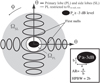 |
Fig. 1 2D projection of the power beam pattern (θ is the zenith angle and ϕ the azimuth) showing the separation between the primary-lobe region ΩPL (inner dashed circle) and the side-lobe region ΩSL (grey ring) with a generic beam pattern pointing at zenith. The angle θ1stnull,min (Eq. (4)) separates the two regions. The exceeding part of this asymmetric primary lobe is considered in the ΩSL region. The black ellipse represents the primary lobe above −3 dB and the ellipse parameters FWHM and AR are defined in the inset box. |
3.5 Computation of the cost function: SLL and SLP
The beam regions are represented in Fig. 1, which shows the case of an elliptic primary lobe, slit into the inner primary-lobe region ΩPL (white circle) and the side-lobe region ΩSL (shaded area). The SLL corresponds to the strongest side lobe over all the ΩSL down to the horizon, whereas the SLP is defined as the integral of the beam in ΩSL (see Eq. (3) for justification).
For the two algorithms, the primary-lobe region ΩPL was delimited by the zenith angle θ < θ1st null, where θ1st null marks the zenith angle of the pattern first null, derived from the first-order derivative along θ. Beyond the first null, we defined the side-lobe region ΩSL. If the primary lobe is not symmetric in azimuth ϕ (e.g. elliptic, due to an elliptic element distribution), the position of this first null varies and can be different various azimuth ϕ. To penalise the asymmetry of the primary lobe, we digitally imposed the definition of ΩPL to take the lowest value of θ1st null over all azimuth ϕ:
![Mathematical equation: $\theta \le {\theta _{{\rm{1st}}\,{\rm{null,}}\,{\rm{min}}}} = _{\phi \in \left[ {0,2\pi } \right]}^{\min }\left( {{\theta _{{\rm{1st}}\,{\rm{null,}}\,{\rm{min}}}}\left( \phi \right)} \right).$](/articles/aa/full_html/2023/04/aa43861-22/aa43861-22-eq7.png) (4)
(4)
For elongated element distributions, the primary lobe is elongated and a fraction of it is counted in ΩSL rather than in ΩPL. As a result, we can predict that the minimisation of SLL and SLP will tend to enforce symmetric patterns without the need to implement additional constraints on the primary-lobe AR.
3.6 Exploration of the tile parameter space
Due to the complexity of the parameter space (e.g. elements number and location), we illustrate the impact of the element pattern (fiso and fdip) on the tile response for two boundary cases of Nant = 5 and Nant = 22 in Sect. 3.6.1. Subsequently, in Sect. 3.6.2, we compare how the figure of merits depends specifically on Nant and how sensitive the results are, depending on the optimisation method used. We analyse the impact of Nant on the SLL in Sect. 3.6.3 and the impact on the tile beam shape in Sect. 3.6.4. Finally, in Sect. 3.7, we give a summary of the obtained solutions and discuss them against the constraints of digital versus analogue phasing.
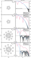 |
Fig. 2 Optimal element distributions and their associated beam pattern profiles for Nant = 5 and Nant = 22 with the two element beam patterns fiso and fdip (from a to d). Left column: element positions in wavelength units. The black dots and the circles represent the element positions and the footprints of their effective area accounting for the minimal distance, respectively (Appendix A). Right column: Normalised power patterns. The red line is the beam profile where the maximum SLL has been located. The blue line is the profile where the maximum SLL is located on the optimal solution. The grey lines are the superimposed pattern azimuthal profiles sampled with 20° steps. The vertical dashed line locates the θ1s null, min (Eq. (4)) and the horizontal dashed line marks the SLL. |
3.6.1 Optimal distributions of elements for Nant = 5 and Nant = 22
Panels a–d of Fig. 2 display examples of the final optimal distributions (left) and the corresponding normalised power beam pattern (right) for the Nant = 5 and Nant = 22 cases, both with the element patterns fiso and fdip. Each element optimal position is represented with a circle of diameter dmin, representing the minimal distance between the elements, as well as the 2D footprint of the element effective area evaluated at zenith at wavelength λ (see Appendix A). The normalised power beam patterns are plotted as a function of θ. Azimuth profiles were sampled every ∆ϕ = 20° and are stacked in grey, and the black line profile is where the maximum SLL is located. Information such as the maximum reached SLL and AR is reported in each plot.
In all four cases, the SLL was reduced compared to the original beam pattern with random initial distributions. and consequently, the HPBW was enlarged. The optimal element distributions are found to be relatively compact and present some circular symmetry. They are associated with a symmetric primary lobe with an AR of ~1.
We consider, in the case of Fig. 2b, that the power diagram is composed of the primary lobe only (SLL ≪ −100 dB) down to the horizon. Observations of the array shape during the run showed that, while the elements were moving and getting closer to one another, the side lobes present in the visible region were ‘expelled’ from this region. The optimal distributions obtained with the two element patterns are identical for Nant = 5 (despite being randomly rotated due to initial and/or final conditions) and they are relatively close, but distinct, in the Nant = 22 case. The difference between the two distributions at Nant = 22 is the arrangement symmetry of the inner elements. In the array of Fig. 2d, no clear symmetry can be observed, while in Fig. 2c, one axis of symmetry (~parallel to the X-axis) exists, as well as an almost three-fold symmetry of 120°.
The difference in individual element beam patterns (fiso and fdip) does not directly explain the difference between the SLLs in Figs. 2c and d. Indeed, the maximum SLL of Fig. 2c is located at θ ≈ 38°, the value of the ideal dipole power pattern in this direction being 0.62 (i.e. 62% of the maximum value at zenith). If we use the same array distribution as in Fig. 2c but with the other element pattern, fdip, the SLL value only changes from −25.6 dB to −27.7 dB in Fig. 2d, compared to −31.1 dB in Fig. 2c. Therefore, the relative distribution of elements plays an important role in the array’s SLL compared to the effect of the element pattern.
Conversely, if we compute the power pattern of the array of Fig. 2d with fiso, large side lobes appear close to the horizon (θ ≈ 90°) and the SLL increases to −17.32 dB. This shows that during the optimisation with fdip, the ‘undesired’ powerful side lobes are being ‘pushed away’, towards the horizon, where fdip is known to take lower values (whereas they must be pushed further away in the invisible region with fiso). One important aspect of this experiment is that the two element patterns, fiso and fdip, constrain the optimisation differently.
Some elements in the inner part of the distribution may occupy positions that generate far side lobes (in the array factor), which dampen as fdip tends to zero at the horizon, resulting in low SLL values. With fiso, the array factor is not dampened by the element pattern down to the horizon (fiso = 1, ∀θ). As a result, the SLL reduction will be more constrained by the relative positions of the elements in the distribution and lead, in the case of fiso, to a distribution of elements presenting some symmetry. From these four cases, we infer that the irregularity and, to a certain extent, the overall symmetry of the element distribution in the central part of the distribution, are necessary conditions to obtain low SLL and a symmetric primary lobe. At this stage, and depending on the optimisation algorithmused, the convergence to a solution and the unicity of the obtained solutions are not guaranteed. This is discussed in the next section, with a quantitative analysis conducted for all values of Nant and the two algorithms.
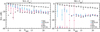 |
Fig. 3 Values of SLL obtained with the two algorithms (SA and KOGAN) using the two element beam patterns fiso (left) and fdip (right). Each circular point is the mean and σ over Ninit = 10 runs. Values for the initial random distributions are plotted with the open circles. Values for the optimised distributions are shown by black filled circles for the KOGAN algorithm and light grey filled circles for the SA algorithm. The dotted line is the best fit of SLL values of the initial random distributions. The stars represent the best solutions obtained over the results of the two algorithms. The arrows indicate out-of-scale values (i.e. cancellation of side lobes). The hollow square represents the maximum SLL of −11.3 dB (with fiso) and of −14.4 dB (with fdip) in the case of a 4 × 4 tile with an element spacing of λ/2. |
3.6.2 Variations in the tile beam shape with Nant
We conducted the optimisation of a tile composed of 𝒪(10) elements (from Nant = 5 to 22) using the two algorithms defined above. For each value of Nant, Ninit = 10, initial random distributions were optimised in order to study the statistical distribution of the solutions. In Sect. 3.6.3, we analyse the effect of Nant on the SLL performance, while in Sect. 3.6.4 we focus on the morphology of the resulting primary beam.
3.6.3 Side-lobe levels versus Nant
Figure 3 presents the resulting SLL values of the power diagram after optimisation of tiles using isotropic (fiso) and ideal dipole (fdip) elements. The SLL is expressed in dB computed from a normalised power pattern (therefore, removing the effect of increasing the number of elements). As a matter of comparison, we also overplotted the initial mean and standard deviation (hereafter σ) values for the SLL of the initial random element distribution (hollow circles) and error bars. The other points (filled circles) are the final mean values and the σ computed over the Ninit element distributions. The occurrence of identical element distributions is high when the error bars are small.
For both element beam patterns, fiso and fdip, the dashed line is the best linear fit on the SLL mean value of the initial random distributions. With an increasing value of Nant, we can see that the SLL, computed over the random initial distributions, decreases linearly by ~10 dB from Nant = 5 to Nant = 22, which confirms the previous result seen in Fig. 2. From Lo (1964), Hendricks (1991), and Steinberg (1972), we can derive that this value decreases approximately with Nantα, with α ≈ −0.5 at low values of Nant. The effective values of α, extracted from Fig. 3 (left and right), are respectively −0.53 and −0.49, showing the agreement with this power law. This decrease depicts the ‘natural’ decrease in the SLL as the number of elements increases. In all cases, both algorithms successfully managed to converge to solutions with a lower SLL (on average), which depends on Nant. We note that specific values of Nant (especially for low Nant values) provide a larger reduction of the SLL than their neighbouring values, potentially marking some ‘magic’ optimal number of elements under our constraints.
In the case of an isotropic element pattern, the SLL levels obtained with KOGAN smoothly decrease with Nant by 2 dB to ~15 dB compared to the initial value, and meet a plateau shared with that of the SA algorithm at high Nant. In the interval Nant < 12, the difference between the two algorithms ranges from 2 to 20 dB, whereas for Nant > 12, the difference in the mean values is ≤5 dB. For the SA algorithm, the σ decreases slowly with Nant, while remaining fairly constant with KOGAN.
In the case of the dipole element pattern, for Nant ≤ 12, both the mean and σ strongly fluctuate, and for Nant > 12, both values vary smoothly with Nant. Differences between the two algorithms are clear as shown by the arrows, telling us that optimal solutions were reached mostly with the SA algorithm (usually with cancelled side lobes). For Nant > 12, the improvement of the mean SLL is steady for both algorithms and is around 10–25 dB below the initial value. The values of σ are also comparable (except for Nant = 14, 16, 17, 18).
The variation in SLL with Nant is smoother in the isotropic pattern case than that in the dipole antenna case. For an isotropic pattern, the side lobes are not cancelled out down to the horizon. As a consequence, the level of the far side lobes raised the minimum achievable SLL. The number of elements Nant has an important effect on the structure of the solution space where high Nant values are associated with more local minima. For Nant > 12 with both element patterns, similar values of SLL indicate that the same element distributions were found with the two algorithms. These solutions may be global minima reached by the two algorithms, or local minima to which they have both converged. As the definitions of the CFs are different, it is more likely that the two algorithms, by evolving on two different spaces, independently reached similar solutions that seem to be the global optima for this range of Nant.
In Figs. B.1 and B.2 are plotted the 2D distributions of the solutions obtained respectively in the isotropic case and the dipole case. All plotted distributions minimise the SLL and are associated with asterisks in Figs. 3 and 4. Depending on Nant, they were obtained either using the SA or the KOGAN algorithm. Given the initial constraints of optimisation, one can derive the following general properties from Fig. B.2.
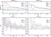 |
Fig. 4 Values of the HPBW (top) and AR (bottom) obtained with the two algorithms (SA and KOGAN) using the two element beam patterns fiso (left) and fdip (right). The conventions are identical to those of Fig. 3, except for the star symbol, which represents the maximum encountered HPBW value with both optimisation methods, and the horizontal dashed line, which represents a symmetric primary lobe with AR = 1. The hollow squares represent the HPBW values of 13° (left) and 12° (right) for a 4×4 tile with an element spacing of λ/2. For this tile the AR is always equal to one. |
3.6.4 Beam shape versus Nant
The reduction of the SLL comes with a widening of the primary beam, as explained in Appendix B.2.1. Figure 4 presents the HPBW and AR values of the resulting power diagrams. The figure follows the same standards as in Fig. 3. The maximum value of HPBW, for all algorithms, and the minimum value of SLL, are represented with asterisks.
In Fig. 4, the statistics over HPBW and AR are presented with the same conventions as in Fig. 3. The mean HPBW values of initial random distributions appear to be independent of Nant, whereas the mean AR decreases significantly with Nant. This is due to the fact that the HPBW of a uniform element tile is proportional to λ/D (with D being the diameter of the tile) and does not depend on the number of elements that compose the tile. Conversely, the relative positions of the elements strongly impacts the shape of the primary lobe, especially at low Nant where the location of each element contributes a lot to the beam pattern morphology. From 2D random distributions with low Nant, the primary beam is expected to have initial values of AR larger than one. These values tend to be reduced as Nant increases, because the disk in which the initial distributions are drawn become filled by more and more elements, lowering at the same time the statistical contribution of the location of one particular element.
With the isotropic element pattern, the solutions obtained with the two algorithms for Nant < 10 provide no side lobe in the visible region, and therefore come with the widening of the beam depicted in Fig. 4. In Fig. 4 (left), we can see a difference between the range Nant < 10 and Nant > 10. For Nant < 10, the final solutions found with the SA algorithm bring a much larger HPBW than that obtained with the KOGAN algorithm. However, in the Nant > 10 range, the HPBW improvements become smaller with increasing Nant. In addition, the values obtained with the SA algorithm are systematically larger by ≈5–10° than those obtained with KOGAN. In Fig. 4 (left), mean and σ AR values with the SA algorithm are higher and evolve more erratically with Nant than those of KOGAN, and can even sometimes overcome the initial value.
In the case of the dipole element pattern, in Fig. 4 (right), we have a clear regime separation between the Nant < 10 and Nant > 10 ranges. For Nant > 10, the HPBW values obtained with the two algorithms follow the same trend with Nant and correspond to the analogue tile size. For Nant < 10, SA gives systematically better HPBW values. The differences in the HPBW values obtained with KOGAN and SA are due, at least in part, to the two different definitions of their CF. To a certain extent, it is possible to minimise the SLL without interfering with the size of the beam, whereas the minimisation of the SLP imposes the widening of the primary lobe (Appendix B.2.1). However, high values of HPBW obtained with the SA algorithm sometimes come at the cost of the beam symmetry. Indeed, an element distribution that minimises the SLL may maximise the AR (e.g. Nant = [7, 8, 9]) if, for example the element distribution is closely packed but elongated in a particular direction. Conversely to Fig. 4 (left), Fig. 4 (right) presents a range of Nant where the two algorithms show close performances. The low AR σ values in Nant = [11, 16] show that the two algorithms have reached to the same optimal element distributions (over the 10 runs) that provide a symmetric beam.
The main difference between the isotropic and dipole element patterns are clearly seen with the zenith angle. The decrease in the dipole pattern to zero down to the horizon seems to help KOGAN and SA converge to reproductible solutions (i.e. lower error bars in Fig. 3) with similar SLL reduction. In the case of the isotropic pattern, SA seems to give systematically better solutions with a larger HPBW than KOGAN for the entire range of Nant. In addition, at θ = 90°, |fdip| equals one, whereas |fiso| equals zero. Therefore, for both element patterns, the HPBW σ is larger at low Nant than at high Nant, because as the array increases in size, the corresponding beam pattern has a thinner primary lobe that is less subject to the particular variation of the element pattern at high θ values.
3.7 Results of the tile study
3.7.1 General shape of optimal element distributions in tiles
At each Nant, the solutions for fiso and fdip seem to follow the same structuring rules, except for some special cases (e.g. for Nant = 8, 10, 12 in Fig. B.2). These particular distributions are optimised for SLL, and since the two CF do not include any explicit constraint on AR, there is no reason for them to present symmetry. Reproducibility of the complete set of possible optimal solutions is rather impossible to guarantee, due to the high number of free parameters brought by Nant. However, for small Nant values, we could reproduce the same solutions with good confidence.
The optimal distributions are irregular. This property appears indeed necessary to avoid grating lobes and strong side lobes (that appear in the presence of any regularity). Using the interferometric approach (Appendix B.1.1), by decomposing the array in pairs of elements (i.e. in baselines, each associated with one (u, υ) spatial frequency), we can highlight the differences between regular and irregular arrays. In regular arrays, the large redundancy of identical baselines provides the same (u, υ) components that are associated with the sensitivity of the same spatial frequencies of the observed target. This results in constructive interferences, whose ‘weight’ will dominate the other spatial contributions. In the array factor, this promotes the presence of grating lobes that are as powerful as the main lobe (which is, itself, the grating lobe situated at the array phase centre). In irregular arrays, with low redundancy, the (u, υ) space is richer in various (u, υ) components and provides a better sampling of the Fourier transform of the aperture autocorrelation. The resulting beam pattern shows no grating lobes and a relatively low level of side lobes.
The optimal distributions are compact. As mentioned above, the overall size of the array conditions the HPBW. With compact element distributions, one ensures the widest primary beam. However, due to the distance limit between elements (Appendix A), a small dense tile arrangement presenting high compacity comes with the risk of bringing high internal regularity (as in a crystal mesh) because of the limited number of possible packed arrangements of the elements (see Fig. B.2 for Nant = 7 and Nant = 15 to 20). The compacity of the array reduces the length of the longest baseline, resulting in a decrease in the angular resolution of the array (i.e. a wider primary beam). Some ‘optimal’ distributions present a structure in two parts, an internal ‘core’ surrounded by a circular ring of elements (see Fig. B.1 for Nant = 7 and Nant = 16, and Fig. B.2 for Nant = 17, 18). The compactness of optimal arrays can be justified from the Fourier relation between the aperture of the distribution and the HPBW (as stated in Appendix B.1.1). Indeed, if a wide Gaussian primary beam is desired, it is only achieved by forming an element distribution that tends to a continuous or compact Gaussian coverage. Since the number of elements is limited, no such aperture filling is possible. Nevertheless, thin Gaussian beams can be approached by using enough elements distributed over a large surface to sample a Gaussian aperture, or using non-uniform weighting. Our optimal tile arrangement should work with broad-band elements. As the wavelength changes quickly across the band, and the compacity depends on the minimal distance between elements, a compromise has to be found to limit the overlap between the element effective areas. The optimal array should be scaled with respect to the optimal wavelength, λopt, which will split the part of the band where the effective area overlaps (λ > λopt), so that where the tile is not seen as compact (λ < λopt).
The optimal distributions present symmetries. Some solutions present axial symmetry or ‘pseudo’ axi-symmetry properties. As we imposed that the HPBW be large and symmetric, and that they present a low SLL, the resulting distributions are roughly circular. The combination of array irregularity with this circular symmetry results in arrays that cannot be superimposed to themselves by any rotation Rϕ ≠ 2π (see Fig. B.1 for Nant = 8, 11, 15). Some other solutions (see Fig. B.2 for Nant = 5, 6, 7, 16, 19) rather present axial symmetry (from one to three axes). At low Nant, it is difficult to form an irregular array that provides a symmetric primary lobe with only a few elements (indicated by the large initial values of AR in Fig. 4). Even if a condition on the AR is not implemented explicitly in the SLL and SLP, their definition enforces the circularisation of the beam (Fig. 1), leading to a compact regular distribution at low Nant.
By examining the distributions from Nant = 12 to 17 in Fig. B.1, we can identify the distribution with Nant = 16 as the one where a sufficient number of elements is ‘profitably’ distributed in the tile (and giving the best SLL in this range of Nant). As Nant increases from 12 to 15, the corresponding distributions converge to the Nant = 16. Each new added element seems to occupy the location where it appeared to be missing in the preceding distribution. This suggests that there could be some optimal number of elements that lead to improved array characteristics. Figure B.2 presents an analogue behaviour in the same interval of Nant.
One can also notice that the element distributions with Nant = 20 in Fig. B.2 and Nant = 18, 19 in Fig. B.1 can be considered as the merger of two ‘elementary’ tiles. Generally, the distributions with large Nant (Nant = 16, 17) often seem to enclose the ‘core’ distributions, such as the one with Nant = 7. These two observations may underline that for specific elements numbers, the optimal distribution (at large Nant) is composed of the assembling of distributions found at lower values of Nant. Conversely, Nant = 9 in Fig. B.1 and Nant = 8, 10, 12 in Fig. B.2 show little or no symmetry. This is again probably due to the lack of an explicit minimisation constraint on AR in the CF definition. The corresponding primary lobe is asymmetric, as depicted in Fig. 4.
3.7.2 Optimal element distribution for NenuFAR analogue tiles
As shown in the previous section, we could find ‘optimal’ element distributions in the range Nant = 5 to Nant = 22. The irregularity of such solutions guarantees a minimum SLL and a wide tile beam, increasing the instrument FOV. Real tile implementation usually includes dipoles with element patterns comprised between isotropic (fiso) and dipolar (fdip) extreme cases. Therefore, the previous optimal distribution can be used to optimise the tile response at zenith and towards some azimuth on the horizon.
For the next generation digital radio telescopes containing >100 000 broad-band elements, such as SKA-LOW, a two-stage hierarchical layout helps to reduce the computational effort and energy consumption, compared to complete element digitisation. As these facilities use broad-band elements (i.e. 10–100 MHz), their signal must be phased and combined with a local analogue beamforming system at the tile level. A large number of directions should also be electronically reachable, and therefore a lot of analogue delays should be applied to the element signals for accurate beamforming.
An irregular tile requires a costly analogue phasing system where Ndelay lines = Nant. In a regular array, however, delay lines can be grouped to phase up pairs of elements (as depicted in Sect. 2.3). Regularity in the tile, enabling the same signal streams to be grouped in mutualised delay lines, represents cost reductions, especially if the tile is replicated several hundred times. The principle of delay lines is beyond the scope of this paper but we refer the interested to van Haarlem et al. (2013) and Girard (2013).
Practical implementation of the tile layout and the analogue phasing strategy impose the choice of a more symmetrical and more regular distribution of elements within the tile, close to the optimal ones defined before. One reasonable choice from our previous study would have been the Nant = 16 solution. The closest regular solution that matches the features of the optimal solution is a regular array sharing the seven central elements in a hexagonal tile: one central element surrounded by two concatenated hexagons, for a total of 19 elements arranged on a equilateral mesh. This solution has a lot of symmetries and a regular pattern, and thus has grating lobes but inherits some FOV properties from the irregular optimal solution. The tile layout shown in Fig. 5 is the one selected for the design of the NenuFAR tiles (Zarka et al. 2012, 2015, 2020). When NenuFAR construction is complete, it will consist of 96 19-element hexagons (hereafter hex19) tiles and six extended tiles to improve the (u, υ) coverage of the whole instrument.
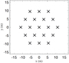 |
Fig. 5 Hexagonal distribution of 19 elements selected for the NenuFAR array. A central element is surrounded by two concentric hexagons. Each element was chosen to be 5.5 m apart (to minimise the effective area overlap). |
4 Impact of the layout and distribution of tiles on the instrument response
In the second part of this study, we evaluate the impact and potential advantage of using the 19 element hexagonal tile compared to using the classical 4 × 4 (hereafter sq16) tiles, used in the LOFAR HBA or the MWA. We study, in particular, the impact of randomly rotating the frame of the tile to mitigate grating lobes coming from the tile regularity.
4.1 Study parameters
First we defined an array of Ntiles (Ntile ~ 100, as in LOFAR-HBA international stations or the MWA) with random positions and rotation angles. We drew a large number of such random arrays, and for each of them we compared the same two CFs (SLL and SLP) of the whole instrument response composed of hex19 or sq16 tiles. This led to inconclusive results, as the ‘noise’ introduced by the vast randomness of possible tile distributions was larger than any noticeable differences between the two types of tiles.
Therefore, we defined a specific distribution of tiles with good aperture coverage characteristics inspired by Conway’s spiral distribution (Conway 1998, 2001) to get a reasonably uniform interferometric baseline distribution (i.e. a uniform (u, υ) coverage). Figure B.3 presents the instrument array under test, made of successive rings surrounding a central tile. The concentric rings include between five and 14 tiles, and their radii follow a geometrical progression and are rotated from each other so as to mimic spiral arms without any symmetry. We explored the range of Ntiles = 6, 12, 19, 27, 36, 46, 57, 69, 82, 96, each with a distribution ensuring a non-redundant (u, υ) coverage without large side lobes in the corresponding dirty beam. For this study, arbitrary lengths between tiles were used with no restriction or control of tile overlapping.
Firstly, we investigated the effect of tile rotation on the array response. Secondly, we quantified the robustness of this effect with different stepping of the rotation angle between tiles. Thirdly, we compared the impact of tile rotation with hex19 tiles and sq16 tiles.
4.2 Results
4.2.1 Qualitative effect of hex19 tiles rotation on instrumental response
We first illustrate the effects of rotating (or not) the layout of the hex19 with respect to other tiles. As we wanted to keep the same polarisation measurements, only the layout was rotated by an arbitrary angle while the was kept element parallel over all the instrument (this can lead to inter-element mutual coupling that may vary from one tile to the other). We simulated Ntiles = 96 at the highest observing frequency of NenuFAR (i.e. 80 MHz), which corresponds to the worst-case scenario as a large number of grating lobes of the tile enter the instrument FOV while having a quasi-random distribution of side lobes and a small HPBW. We studied two pointing directions: the local zenith (θ = 0°), and a low-elevation direction (θ = 70°). Both the full instrument and the tile were electronically pointed towards these two directions.
The comparison between rotated or not rotated is seen in Fig. 6 (in the top four panels for the zenith pointing, and in the bottom four panels for the low-elevation pointing). Each line of Fig. 6 presents the stacking of 2D cuts of the instrument beam pattern at 0.5° resolution, in parallel planes of azimuth ϕ = 0° or ϕ = 90°. Each plot shows the stacked beam profiles along with the maximum SLL. In the left column, the tiles were not rotated with respect to each other, while in the right column, they were rotated by an arbitrary angle (with 1° steps). The grating lobes of the hex19 tiles can clearly be seen and play the role of an envelope for the side lobes of the instrument array factor. On the right, the effect of rotation translates as an overall increase in the average SLL, but this average is always lower than that induced by the tile grating lobes.
When the instrument and tiles are pointed at low elevation, the distribution of the ‘background’ side lobe forest and grating lobes changes dramatically (with respect to the zenith pointing) when the tiles are not rotated, whereas these variations are smoothed out when the tiles are rotated. This means that, in order to guarantee a steady instrument directional gain with respect to the background, rotation of the tiles is mandatory to lower the effect of tile analogue pointing. The decrease in SLL is between 4 and 6 dB for both pointing directions, and the average SLL (computed on the 100 brightest side lobes) is respectively around 6 and 7 dB for both directions. Qualitatively and quantitatively, we can see that tile rotation is necessary to lower the effect of the tile beam pattern on the whole instrument response.
Following the same example, we can now determine the minimal angular step of tile rotation to achieve such an SLL reduction at ν = 20, 40, 60, and 80MHz. In Fig. 7, each panel represents the reduction of the maximal SLL as a function of the angular rotation step between tiles for both the zenith and low elevation. While at ν = 20 MHz, no improvement can be seen, the three other frequencies display plateaus up to a maximum step at which the effect of tile rotation drops. For example, at ν = 80 MHz, 10° rotation steps imply no significant loss in SL reduction efficiency. Thus, rotation steps of 10° are as efficient as angular steps of 0.01°. This relaxes the constraint on the accuracy of the tile rotation with respect to when installed on the field.
4.2.2 Comparing hex19 and sq16
To get a general idea of the effect of tile rotation depending on the size of the array, we conducted studies over Ntiles = 6, 12, 19, 27, 36, 46, 57, 69, 82, 96 and plotted the variation in the maximum SLL at f = 80 MHz in Fig. 8, and in Fig. 9 we plotted the side-lobe power fraction ΩSL /ΩA in percentages, that is to say, the fraction of power in all the sky, excluding the main beam region of size 2λ/D around the pointing direction. The left and right columns depict, respectively, the results when the tiles are not rotated or rotated, and the symbols refer to sq16 (black triangles) and hex19 (red squares).
For each number of Ntiles, for pointing directions different from zenith, we plot the SL levels in Figs. 8 and 9 for 12 different azimuths.
The main effect of tile rotation resides in an improvement of the SLL by ~1–10 dB for both hex19 and sq16 designs, for all pointing directions and for various values of Ntiles. It is when the number of tiles is ≤80 that the highest SLL reduction is achieved. When pointed at zenith, the effect of the grating lobes is clearly damped, whereas for low-elevation pointing, the tile rotation only makes the SLL uniform along all azimuths at roughly the same level as without rotation. For certain values of Ntiles, rotated sq16 tiles sometimes outperform hex19 tiles.
However, in all cases, the hex19 tiles always have the lowest fraction of power in the main lobe compared to the sq16 tiles. As a consequence, the hex19 tiles make the instrument less impacted by isolated RFI and background noise. In addition, we see that around Ntiles = 20–30, the ratio reaches a minimum, suggesting that a modest instrument can already provide a fair sensitivity and a smooth beam. When the tiles are rotated, the distribution of power is less azimuth dependent, meaning that the pattern becomes more circularly symmetric. The improvement effect is more visible for a small number of tiles, and tends to make the behaviour uniform at the various azimuths. Indeed, rotating the tiles not only reduces the (average) SLL, it also circularises the synthetic array beam.
5 Conclusion and discussion
We have presented the results of the 2D optimisation of small element arrays that minimises their SLL and maximises their HPBW. This optimisation was carried out in the visible space only and with arrays pointing at zenith and at low elevation.
5.1 Optimal distribution properties
We first used a modified deterministic algorithm (KOGAN, Appendix B.1.1) and a modified simulated annealing algorithm (SA, Appendix B.2.2) to address the optimisation in two different ways. We found solutions that minimise the SLL, and offer a wide (a large value of HPBW) and symmetrical (AR value close to one) primary beam. Optimal tile distributions are found to be irregular and compact, and to present elements of symmetry. We have also noticed that the solutions at high Nant can sometimes be decomposed in solutions of lower Nant (e.g. the distribution with Nant = 7 is included in that with Nant = 16 in Fig. B.1, and portion of the distribution with Nant = 16 included in Nant = 20 in Fig. B.2). This behaviour suggests that some specific numbers of elements (e.g. Nant = 7 and Nant = 16) form a ‘basis’ in the solution space defined by our constraints. We display optimal tile distributions with Nant = 5 to Nant = 22 elements. We obtained optimised distributions of elements suitable for digital beamforming (or analogue beamforming with one delay line per antenna) in a small element tile. However, optimal solutions lead to arrays that are expensive to phase with analogue systems because of their lack of regularity, which makes analogue phasing systems cheaper (see Sect. 2.3). Thus, we proposed a compromise, hex19, which displays a regular pattern using an equilateral lattice that was selected for NenuFAR. The triangular lattice presents statistically fewer grating lobes in the sky than a square lattice Mailloux (2005) and Wayth et al. (2018). We compared the performance of hex19 to that of sq16 within a simulated tile arrangement in a whole instrument composed of Ntiles = 6 to 96. Relative random rotations at 10° helps to mitigate the maximum SLL by reducing the impact of grating lobes in the array response, and while the rotation present advantages with both hex19 and sq16, hex19 will cause less contamination by isolated RFI and background noise. In addition, the regularity of the hex19 tile presents the serious advantage that only ten delay lines (per polarisation) are required to form the phasing system that enables the tile to point anywhere in the visible sky. Indeed, we need ten delay lines to fully phase the hex19 and sq16 tiles towards any direction in the sky, but we benefit from 20% more elements and fewer side lobes with hex19. As the cost of an analogue tile is largely dominated by the cost of the broad-band analogue phasing system (cable lengths, and electronic summation cells and relays), the performances of hex19 significantly overcome those of sq16 for essentially the same cost.
This hex19 tile is now used as the building block for the NenuFAR array (both a LOFAR ‘super station’ and a large standalone low-frequency radio telescope – beamformer & interferometer – presently reaching the final construction stage at the Nançay Radio Observatory around the LOFAR FR606 station (see Zarka et al. 2012, 20201; Girard et al. 2012). It should be noted that the Focal L band Array for the Green Bank Telescope (GBT/FLAG, developped by the NRAO and Brigham Young University) is a focal plane array that was independently designed as a hexl9 tile (see Roshi et al. 2017, 2018; Rajwade et al. 2018). The ‘kite’ phase array feed (PAF) is also constituted by an hexagonal array of 19 dual-polarisation dipole elements connected to cryogenised LNAs fed to a multi-beam pointing system. In the GBT case, the array beam shape was optimised to increase both the sensitivity and the radial symmetry to the ~20′ FoV of the antenna. In particular, the element spacing arranged in a hex19 tile (12 cm, 0.56λ at 1.4 GHz Roshi et al. 2017) enabled the formation of seven beams in the GBT FOV, angularly spaced by a half-power beam width. As a result, with the PAF size, the element size, and the relative distance, seven high-sensitivity beams can be formed to pave the antenna FOV, thus increasing the survey speed for the scientific programmes of the GBT. Our study provides a firm theoretical basis for this tile topology.
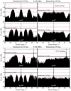 |
Fig. 6 Beam pattern profiles for an instrument with 96 tiles, for zenith observations (four top plots) and low-elevation pointing (four bottom plots). Each group of four plots shows the stacking of 2D profile cuts of the beam pattern (cuts parallel to azimuth ϕ = 0° (left column) and ϕ = 90° (right column)). The envelope associated with the grating lobes of the tile limit the level of the instrument side-lobes array factor. Rotating the tiles helps lower these strong grating lobes envelope and smooth the SLL around a constant level that is likely independent of the pointing direction. |
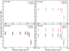 |
Fig. 7 Maximum SLL level decreases (in dB) induced by tile rotation, as a function of the angular rotation step at four frequencies: 20, 40, 60, and 80 MHz (left to right and top to bottom). Points and error bars for each rotation angular step are plotted for zenith pointing (black), and for low elevation pointing (red). Top left: all values are null because no SLL could be detected at f = 20 MHz. |
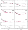 |
Fig. 8 Maximum SLL as a function of the number of tiles and pointing direction θp = {0°, 30°, 60°}. The sq16 (black triangle) and hexl9 (red square) converge to similar results when the tile rotation is applied. |
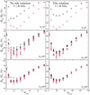 |
Fig. 9 Fraction of power beyond the primary beam as a function of the number of tiles and pointing direction. The style of the data points is the same as in Fig. 8. |
5.2 Convergence of the algorithms
Both the KOGAN and SA algorithms have advantages and drawbacks, depending on the number of elements and the topology of the chosen CF. The Kogan algorithm generally produced symmetrical distributions with low AR values (Fig. 4), whereas the SA algorithm converged to distributions providing larger HPBW values (Fig. 4). A more extensive statistical study at each Nant (with >1000 random initial distributions) could be performed to improve the exploration of the CF space, and therefore of the solution space. This could help to qualify these solutions as local or global minima. But the solutions proposed here are already operational and provide very low SLLs and good pattern characteristics.
The different cooling strategies (for SA) and different gain values (for SA and Kogan) can modify the convergence of the algorithms. However, the values of these parameters may not be adapted for all values of Nant. It is the same if a stopping criterion is defined for both algorithms. This criterion may not be adapted at different Nant values, depending on the speed of convergence in the CF space having different topologies. A stopping criterion computed over a small number of iterations may abruptly stop the course of the convergence in a CF space presenting wide plateaus (where the CF variations fall below the limit defined by the stopping criterion) between valleys. In our study, we could raise the morphological trends that optimal solutions seem to provide. Deterministic algorithms fall easily in local minima but provide optimal solutions for small values of Nant. However, the convergence to a global minimum with stochastic methods is only statistical and better solutions can always be found in such a large parameter space.
5.3 Experiment reproducibility
The code used in the optimisation was originally developed on IDL 7.1 and is available online2. A Python implementation is currently being written.
5.4 Limitations
This study focuses on the pattern optimisation brought by the relative arrangement of elements in a continuous 2D space with a uniform weighting scheme (all elements have the same weight in the array response). We focused on the topology of the optimal distributions and not on the efficiency of the two algorithms that were used to produce the results. The mutual coupling between the elements was not taken into account as it highly depends on the radiator geometry, their relative orientations, proximity, the electrical properties of each element, and the ground plane, and would have required a more complex approach involving electromagnetic constraint in the computation of the tile and array response.
5.5 Consequences for the design of large antenna arrays
As we mentioned in the Introduction, large arrays (such as the upcoming SKA1-LOW, Macario et al. 2022) will be composed of >100 000 receiving elements that have to be arranged in sub-arrays. In the current design, a significant number of stations (Ntiles = 512) composed of Nant = 256 broad-band dipoles, represent a tremendous engineering and signal processing challenge. In each SKA-LOW station, all antenna signals are digitally recorded and phased together numerically, which enables a lot of beamforming flexibility. However, cost and power consumption can limit the feasibility of such giant arrays. Special cases of analogue phased tiles and analogue phasing systems, such as HBA tiles or NenuFAR hex19 tiles, can represent a trade-off that could cut the cost, power consumption, and computing complexity, and can be a basis for an alternative solution for SKA1-LOW if the power consumption proves to be too high.
The flexibility of the digital beamforming is unfortunately limited by the present design of the SKALA elements (de Lera Acedo 2012), which has a main beam aperture at 45° maximum zenith angle compared to ~ 70° maximum zenith angle in NenuFAR. This will be a significant limitation for very-wide-field surveys and instantaneous sky imaging. Regular small tiles may bring artefacts and grating lobes that can be mitigated by random relative rotations.
Movies
Movie 1 (2-SA-6elem-fdip-converged) Access Supplementary Material
Movie 2 (3-KOGAN-16elem-fdip-Converged) Access Supplementary Material
Movie 3 (4-SA-16elem-fdip-Converged) Access Supplementary Material
Movie 4 (5-SA-16elem-fdip-slowcooling-notconverged) Access Supplementary Material
Movie 5 (6-SA-16elem-fiso-fastcooling-notconverged) Access Supplementary Material
Acknowledgements
The authors acknowledge the support of the Observatoire de Paris, the CNRS/INSU, and the ANR (French Agence Nationale de la Recherche’) via the program NT09-635931 ‘Study and Prototyping of a Super Station for LOFAR in Nançay’. Support to nenuFAR from Région Île-de-France program DIM-ACAV. Support to NenuFAR from Région Centre-Val de Loire via the Initiatives Académiques de l’Univ. Orléans-Tours. The authors thank Frederic Boone for his useful inputs.
Appendix A Minimal distance between elements
To handle element collision, we defined a minimum distance between the elements to avoid overlapping and also to exclude trivial solutions with collocated elements (having no side lobes coming from the AF), with important effective area loss. Real elements used in phased arrays are mostly dipole-like elements. For that reason, we derived this minimal distance from the effective area of a single dipole, as the minimum distance that avoids effective area loss due to overlap. This distance dmin is then given by:
 (A.1)
(A.1)
With Ωd = 8π/3sr, we obtain  .
.
If the real array has to be optimised over a relatively large bandwidth spanning over [λmin, λmax] (with λmax − λmin ≈ (λmin + λmax)/2), and as Aeff ∝ λ2, the overlap of the effective area becomes large at long wavelengths for dense arrays. This will set the minimal distance dmin ≈ 0.39 λopt.
If λopt = λmin, a large effective area overlapping at low frequency is expected and the total effective area does not scale with λ2 any more.
If λopt = λmax, there are more numerous intense side lobes in the diagram at high frequency; the array is sparse and the primary beam is thin.
Thus, the choice of λopt in [λmin, λmax] is the result of a compromise between the loss of the effective area for λ > λopt and a small FOV for λ < λopt. Once λopt is chosen, it is possible to scale the elements distributions mentioned in this work to a chosen λ.
A.1 Handling antenna collisions
During the optimisation process, elements tend to gather in close-packed clusters (therefore giving a wider synthetic beam) and start to collide at distance dmin. In the two algorithms, each new configuration of elements is checked for collisions. Each colliding pair is geometrically stretched and the two elements are progressively pushed away at a distance ≳ dmin in opposite directions. The optimisation process is temporarily suspended until there are no more colliding elements.
Appendix B Deterministic versus stochastic methods
B.1 Exploiting the derivative of the beam: Kogan’s approach
B.1.1 Kogan algorithm
The long-used software package Astronomical Image Processing System (AIPS; Fomalont 1981) for radio astronomy contains the routine CONFI (Kogan 2000), which optimises the element positions in an interferometer by using the regularity of the synthetic point spread function (PSF) derived. This antenna distribution and the PSF are linked together by the Wiener-Khintchine theorem via the Fourier transform of the aperture autocorrelation (the latter is referred to as the (u, v) coverage). The Kogan algorithm operates in the ‘direct’ space of the elements. Alternate algorithms propose optimising the PSF in the Fourier plane. In Boone (2001, 2002), the density of (u, v) samples as a pressured gas that relaxes on a desired (u, v) model density. This method is not adapted for a low number of elements as there are not enough (u, v) samples to obtain a smooth (u, v) density on a high-resolution grid. Thus, we prefered to implement Kogan’s algorithm, which can work with small arrays.
The principle of the KOGAN algorithm is to use the maximum SLL as its CF and try to reduce it in a restricted part of ΩLS. From the direction u of the strongest side lobe, the value of the PSF in this direction is decreased by imposing physical shifts on the elements parallel to the planar projection uxy of u (considering a (x, y, z) Cartesian frame). The ‘exact’ quantities required to shift the position of the ith element are derived from the first derivative of the PSF in this direction (Kogan 2000):
 (B.1)
(B.1)
 (B.2)
(B.2)
where:
| g | is a gain factor (set to 0.01 λ); |
 |
is the gradient of the power beam pattern P with respect to a displacement of δri in the direction u; and |
 |
is the angle between the x axis and the projected vector uxy. |
The gain factor g enables convergence control and, by making the process iterative, only a fraction g of the displacements are imposed to elements. This gain factor was adapted to the scale of the problem and is equal to 0.01.
B.1.2 Local minima trapping
The deterministic nature of this algorithm implies that, for identical initial distributions of elements, the same final configurations will be obtained. Final configurations may not be optimal ones because nothing prevents the process from falling in the numerous local minima of the solution space. Trapped in a local minimum, the process starts to oscillate by applying small and opposite displacements back and forth.
For each optimisation, the code can stop when the CF variations fall below a predefined threshold, or if it has reached a maximum number of iterations (taken at relatively large intervals namely several times the typical number needed for the code to be trapped in a local minimum). At the last iteration, the best and the final element distributions (not necessarily strictly identical due to the above-described oscillations) as well as their corresponding SLL are stored.
An example of a classical minimisation algorithm is the gradient descent method (Fletcher & Powell 1963) where the optimum search always goes ‘downhill’ according to the direction of the gradient of the CF. From a given starting element distribution, this deterministic downhill search converges towards the nearest local minimum. However, this method is not adapted for reaching the global minimum of the CF, especially if the CF has a complex topology (namely a large number of local minima). Most ‘solutions’ given by this method will be local minima of the CF, likely to be non-optimal solutions.
The probability of converging towards the global minimum can be increased either by performing multiple runs with random initial conditions when using deterministic algorithms (i.e. many random starting positions in the parameter space), or by using stochastic algorithms.
Repeating the operation with different random initial distributions helps us to understand the topology of the CF over the parameter space, and ultimately increases the chances of finding the best solution for each value of Nant. In order to prevent this trapping with the KOGAN algorithm, we ran several (Ninit) optimisations with different initial random element configurations.
B.2 Finding a global optimum with simulated annealing
Another way to achieve global minimisation is to consider stochastic algorithms. They are generally involved in hard combinatorial problems such as the ‘travelling salesman problem’ (Garey & Johnson 1979). Independently of the complex topology of the CF, these methods always statistically (but slowly) converge to the best solution without being trapped in local minima.
We chose the simulated annealing (SA) method (Kirkpatrick et al. 1983) to update and optimise the positions of the elements. This method has already been applied to the positioning elements in linear arrays (Murino 1995). In Hopperstad & Holm (1999), it was used to optimise 2D arrays with elements placed on a discrete grid with a rectangular mesh. In Trucco & Repetto (1996), the distribution of sparse arrays was addressed by optimising both the position and the weight (in a classical beamformer) of the antenna. In the present work, we implemented the SA algorithm in the ‘continuous’ 2D case (namely the elements were placed continuously in the aperture plane). The CF defined for KOGAN can also be used with SA and provides similar solutions to KOGAN (when used with different random initial configurations). Nevertheless, it is preferable to use a CF that is an explicit function of the antenna positions, such as the total power present in the side-lobe region ΩSL.
B.2.1 Minimisation of the SLP
Using the definition of the beam solid angle Ω defined as the integral (Kraus 1984)
 (B.3)
(B.3)
with Pn being the normalised power beam pattern defined in Sect. 2.2 and Ω = 4π/Pn = 4π/G, G being the maximum gain of the beam pattern, we can separate the contribution in the primary-lobe region ΩPL and the contribution in the rest of the element power diagram (the side-lobe region noted ΩSL):
 (B.4)
(B.4)
For a given number of elements, Ω = 4π/Pmax, and at zenith,  . As a consequence, the integral in Eq. B.3 is constant for each value of Nant. Therefore, any reduction of ΩSL leads to an automatic increase in ΩPL. In arrays containing a small number of elements, large values of ΩPL are obtained with ‘compact’ element distributions that produce a wide regular primary beam and a low SLL. As a consequence, the minimisation of the SLL is linked to the minimisation of ΩSL. By defining the CF as the value of ΩSL, these two goals can be attained. This CF cannot be used with KOGAN, which relies, by construction, on the values of local derivatives of Pn to decrease its value in particular directions.
B.2.2 The simulated annealing method
This algorithm is based on the analogy with the slow cooling procedure used in metallurgy to obtain a perfect metallic crystal (without flaws). This method is a thermally controlled Monte-Carlo algorithm whose objective is to minimise the value of the CF (defined in B.2.1) by randomly moving the elements in the 2D plane around their instantaneous positions. The permitted amplitude of motion of the elements (i.e. the relative modification of the CF value) is controlled by a Boltzmann acceptance factor (Metropolis et al. 1953):
 (B.5)
(B.5)
with:
∆CF = (CF)i+1 − (CF)i;
kb, the Boltzmann constant (assigned to an arbitrary value in this context). In our study, kb = 1;
T, the system temperature (which characterises the freedom of the system to explore in the parameter space). T is forced to decrease as the iteration number increases by following a cooling scheme.
Starting from a random initial distribution, the current values of the 2 × Nant element positions are slightly disturbed by a small random quantity (controlled by a gain factor g identical to that of KOGAN, here g = 0.01λ). The new value of CF is tested according to the following rules to accept or reject the new distribution:
if ∆CF < 0 (i.e. a decrease in the CF), the new set of positions is accepted and a new iteration is performed;
if ∆CF > 0 (i.e. an increase in the CF) and U[0,1](x) < b(∆CF, T), the current state is accepted anyway and a new iteration is performed (U[0,1](x) is a random value drawn from an uniform distribution over [0, 1]);
if ∆CF > 0 and U[0,1](x) > b(∆CF, T), the current state is rejected and another random set of displacements is tested.
The method is more robust than a simple downhill method because it permits uphill explorations to ‘escape’ from local minima. Large uphill explorations are first encouraged at high temperature, T, and as the temperature decreases, the system is progressively conditioned to preferably go downhill towards lower minima.
B.2.3 Temperature control
The cooling scheme (the variation of T with the number of iterations) affects the convergence of the process. For each temperature step, the system is considered to have reached its ‘thermal equilibrium’ after a predefined number of successful adoptions of new antenna positions. The temperature is then decreased by a small factor. As the convergence is statistical (as mathematically demonstrated in Rajasekaran 1990), several runs of the algorithm were performed before selecting an adequate cooling scheme. In the study, it was found that a geometric cooling law that consisted in decreasing the temperature by steps of 1%, led to reasonable results. Such step-by-step cooling ensures the convergence of the system.
Two temperature regimes can be defined:
kbT ≫ ∆CF ⇔ b ≈ 1: the system has a high temperature, enabling free uphill and downhill exploration of the CF without being trapped in local minima;
kbT ≪ ∆CF ⇔ b ≪ 1: the system has a low temperature and is statistically confined to go downhill to ‘low-energy valleys’. All variations of the CF are encouraged downhill towards the local minimum, expected to be the global minimum at this stage of the convergence, with little chance of getting outside again. In between, the slow decrease in kbT enables the system to get out of ‘shallow’ minima, whereas it tends to keep going down in deep valleys.
For example, with kbT ≈ 100∆CF, the probability of accepting uphill explorations is about 99%. The probability is only around 37% for kbT ≈ ∆CF and it is reduced to 4.10−5% for kbT ≈ 0.1∆CF. To correctly map the evolution of that probability, we can estimate the initial temperature of the system by taking the average of ∆CF over a limited number of iterations with an arbitrary high-temperature regime (e.g. T = 109 K). The Boltzmann constant can then be modified to adjust the starting ratio  of the Boltzmann factor to tune the convergence process to the range of acceptance probabilities.
To improve the SA algorithm, we implemented the capability to ‘reheat’ the system when required. At temperature T, if the CF did not decrease after a certain number of iterations (e.g. when new element displacements cannot be easily accepted), the temperature was increased by a factor of 10% that ‘reheated’ the system for a limited number of iterations only. With a higher temperature, we raised the probability of uphill CF valley crossing (by lowering the ratio in the Boltzmann term). No change of the gain was performed during this stage. We found that this reheating helped to reduce blocked configurations.
B.2.4 Stop criterion and solution optimality
Convergence of the algorithm can be monitored with the variations of  computed over a sliding window. This quantity is then compared to a threshold value that can stop the algorithm. However, this threshold value, as well as the size of this sliding window, depends on the number of elements. Preliminary tests showed that the values of the CF (with the number of iterations) often formed plateaus that were sufficiently long to trigger the stop of the algorithm without reaching the lowest possible value of CF. To prevent the algorithm from stopping prematurely, we let the algorithm freely evolve until a maximum number of iterations Nequil was reached (it reaches a permanent regime at a given temperature level). This maximum number of iterations was therefore set to Ncoolstep = 5 × 10⁴ iterations to limit the computation time while ensuring a sufficient margin for the convergence. As the iteration-to-iteration variations of the CF are not predictable and depend on the number of elements, we retained the best distributions that presented the lowest SLLs during the run. This solution may not be the one obtained at the last iteration but is a statistical proxy for the probable topology of the best solution.
Our implementation of the SA algorithm incorporating reheating (Sect. B.2.3) was tested against a classical gradient descent minimisation algorithm on the Rastrigin function Mühlenbein et al. (1991). This function is a punitive 2D CF used in the optimisation development as a stress test for any global minimum search. Indeed, this function maps a 2D comb of local minima really close to a central global minima. All minima are separated by ∆x = ∆y = 1. We defined the 2D space in the domain 𝒟 : x ∈ [−10.10], y ∈ [−10.10] but drew random uniform initial starting positions in the sub-space 𝒮 : x, y ∈ [−4.4]2.
By considering N = 100 initial at random starting locations on the Rastrigrin function, and that Ncool step = 5000 and Nequil = 3000 for the SA, we obtained the following results: 100% of the solutions were located in the right valley, as close as ±2.10−3 to the global minimum position; and 25% of them were as close as 3.10−4 to the global minimum. For the gradient descent, initialised at random loci in 𝒮:, 100% of the solutions were in 𝒮, 23% were in the right valley (20% theoretically for a uniform initial distribution in 𝒟), and 5% were as close as ±0.79 from the global optimum. Even if we cannot extrapolate to a higher dimensional where the CF presents a more complex topology, we can safely say that, at worst, our implementation provides better solutions with a sounder statistical weight than a randomly initialised gradient descent.
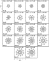 |
Fig. B.1 Optimal tile distributions with |

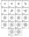 |
Fig. B.2 Optimal tile distributions with fdip from Nant = 5 to Nant = 22. For each value of Nant, the SLL is reported. The same convention as Fig. B.1 is used. |
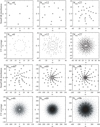 |
Fig. B.3 Tested instrument layouts from Nti1es=6 to 96 following a geometric progression in number of elements and relative rotation to mimic spiral arms. The first and third lines are the tile distributions on the ground, and the second and fourth lines are the corresponding snapshot (u,v) coverage for a zenith observation. |
Appendix C Glossary and notations
| Aeff | effective area |
| AR | axial ratio |
| CF | cost function |
 |
complex electric field |
| ‘H’, ‘E’ planes | principal planes of the antenna |
| fdip | pattern of a dipole with azimuthal symmetry |
| fiso | pattern of an isotropic antenna |
| FOV | field of view |
| G | beam gain |
| g | optimisation control gain |
| HPBW | half power beam width |
| λ, λopt | wavelength and wavelength of optimisation |
| Ninit | number of initial random configuration |
| Nant | number of elements in the tile |
| Ωd | solid angle of a dipole |
| P, Pmαx | power pattern, power pattern maximum |
| Pn | normalised power pattern |
| Rϕ | rotation of angle ϕ in the antenna plane |
| SA | simulated annealing |
| SLL | side-lobe level |
| SLP | side-lobe power |
References
- Balanis, C. 2005, Antenna Theory: Analysis and Design, (John Wiley & Sons), 33 [Google Scholar]
- Boone, F. 2001, A&A, 377, 368 [NASA ADS] [CrossRef] [EDP Sciences] [Google Scholar]
- Boone, F. 2002, A&A, 386, 1160 [NASA ADS] [CrossRef] [EDP Sciences] [Google Scholar]
- Charrier, D. 2014, in 6th International Conference on Acoustic and Radio EeV Neutrino Detection, ARENA2014, Annapolis, USA [Google Scholar]
- Conway, J. 1998, A Preliminary ALMA Zoom Array Design for the Chajnantor Site, Tech. rep. [Google Scholar]
- Conway, J. 2001, Self-Similar Spiral Geometries for the LSA/MMA, Tech. rep. [Google Scholar]
- Davidson, D. 2012, MeerKAT and SKA phase 1, ISAPE2012, Xi’an, China, 1279 [Google Scholar]
- de Lera Acedo, E. 2012, in 2012 International Conference on Electromagnetics in Advanced Applications, 353 [CrossRef] [Google Scholar]
- Dewdney, P., Hall, P., Schilizzi, R., & Lazio, T. 2009, Proc. IEEE, 97, 1482 [Google Scholar]
- Fletcher, R., & Powell, M. J. D. 1963, Comput. J., 6, 163 [CrossRef] [Google Scholar]
- Fomalont, E. 1981, Natl. Radio Astron. Observ. Newslett., 3, 3 [Google Scholar]
- Garey, M. R., & Johnson, D. S. 1979, Computers and Intractability: A Guide to the Theory of NP-Completeness (New York, USA: W. H. Freeman & Co.) [Google Scholar]
- Girard, J. N. 2013, PhD thesis, Observatoire de Paris [Google Scholar]
- Girard, J. N., Zarka, P., Tagger, M., et al. 2012, Comptes Rendus Physique, 13, 33 [NASA ADS] [CrossRef] [Google Scholar]
- Hallinan, G. 2014, in Exascale Radio Astronomy, 2, 10203 [NASA ADS] [Google Scholar]
- Hendricks, W. 1991, IEEE Trans. Antennas Propag., 39, 1757 [CrossRef] [Google Scholar]
- Hicks, B. C., Paravastu-Dalal, N., Stewart, K. P., et al. 2012, PASP, 124, 1090 [CrossRef] [Google Scholar]
- Hopperstad, J. F., & Holm, S. 1999, in International Workshop on Sampling Theory and Applications Proceedings, 91 [Google Scholar]
- Hotan, A. W., Bunton, J. D., Chippendale, A. P., et al. 2021, PASA, 38, e009 [NASA ADS] [CrossRef] [Google Scholar]
- Kirkpatrick, S., Gelatt, C. D., & Vecchi, M. P. 1983, Science, 220, 671 [Google Scholar]
- Kogan, L. 2000, IEEE Trans. Antennas Propag., 48, 1075 [NASA ADS] [CrossRef] [Google Scholar]
- Kraus, J. 1984, Radio Astronomy (Cygnus-Quasar Books) [Google Scholar]
- Lo, Y. 1964, IEEE Trans. Antennas Propag., 12, 257 [NASA ADS] [CrossRef] [Google Scholar]
- Macario, G., Pupillo, G., Bernardi, G., et al. 2022, J. Astron. Telescopes Instrum. Syst., 8, 011014 [NASA ADS] [Google Scholar]
- Mailloux, R. 2005, Phased Array Antenna Handbook, Artech House Antennas and Propagation Library (Artech House) [Google Scholar]
- Metropolis, N., Rosenbluth, A. W., Rosenbluth, M. N., Teller, A. H., & Teller, E. 1953, J. Chem. Phys., 21, 1087 [Google Scholar]
- Mühlenbein, H., Schomisch, M., & Born, J. 1991, Parallel Comput., 17, 619 [CrossRef] [Google Scholar]
- Murino, V. 1995, in 1995 International Conference on Acoustics, Speech, and Signal Processing, ICASSP-95, 5, 3627 [CrossRef] [Google Scholar]
- Prasad, P., Huizinga, F., Kooistra, E. et al. 2016, J. Astron. Instrum., 5, 1641008 [NASA ADS] [CrossRef] [Google Scholar]
- Rajasekaran, S. 1990, On the Convergence Time of Simulated Annealing, MS-CIS (Department of Computer and Information Science, School of Engineering and Applied Science) [Google Scholar]
- Rajwade, K. M., Pingel, N. M., Black, R. A., et al. 2018, in Pulsar Astrophysics the Next Fifty Years, eds. P. Weltevrede, B. B. P. Perera, L. L. Preston, & S. Sanidas, 337, 398 [NASA ADS] [Google Scholar]
- Roshi, D. A., Shillue, W., Fisher, J. R., et al. 2017, in 2017 XXXIInd General Assembly and Scientific Symposium of the International Union of Radio Science (URSI GASS), 1 [Google Scholar]
- Roshi, D. A., Shillue, W., Simon, B., et al. 2018, AJ, 155, 202 [NASA ADS] [CrossRef] [Google Scholar]
- Steinberg, B. 1972, IEEE Trans. Antennas Propag., 20, 129 [Google Scholar]
- Trucco, A. & Repetto, F. 1996, in OCEANS ’96, MTS/IEEE. Prospects for the 21st Century. Conference Proceedings, 3, 1510 [CrossRef] [Google Scholar]
- van Haarlem, M. P., Wise, M. W., Gunst, A. W., et al. 2013, A&A, 556, A2 [NASA ADS] [CrossRef] [EDP Sciences] [Google Scholar]
- Wayth, R. B, Tingay, S. J., Trott, C. M. et al. 2018, PASA, 35, 33 [NASA ADS] [CrossRef] [Google Scholar]
- Zarka, P., Girard, J. N., Tagger, M., & Denis, L. 2012, in SF2A-2012: Proceedings of the Annual meeting of the French Society of Astronomy and Astrophysics, eds. S. Boissier, P. de Laverny, N. Nardetto, et al., 687 [Google Scholar]
- Zarka, P., Tagger, M., Denis, L. et al. 2015, in 2015 International Conference on Antenna Theory and Techniques (ICATT), ICATT 2015, Kharkiv, Ukraine [Google Scholar]
- Zarka, P., Denis, L., Tagger, M. et al. 2020, in URSI GASS 2020: Session J01 “New Telescopes on the Frontier”, 022, https://tinyurl.com/ycocd5ly [Google Scholar]
All Tables
Comparison of the station and tile configurations for a selection of SKA pathfinders, precursors, and demonstrators.
All Figures
|
Fig. 1 2D projection of the power beam pattern (θ is the zenith angle and ϕ the azimuth) showing the separation between the primary-lobe region ΩPL (inner dashed circle) and the side-lobe region ΩSL (grey ring) with a generic beam pattern pointing at zenith. The angle θ1stnull,min (Eq. (4)) separates the two regions. The exceeding part of this asymmetric primary lobe is considered in the ΩSL region. The black ellipse represents the primary lobe above −3 dB and the ellipse parameters FWHM and AR are defined in the inset box. |
| In the text | |
|
Fig. 2 Optimal element distributions and their associated beam pattern profiles for Nant = 5 and Nant = 22 with the two element beam patterns fiso and fdip (from a to d). Left column: element positions in wavelength units. The black dots and the circles represent the element positions and the footprints of their effective area accounting for the minimal distance, respectively (Appendix A). Right column: Normalised power patterns. The red line is the beam profile where the maximum SLL has been located. The blue line is the profile where the maximum SLL is located on the optimal solution. The grey lines are the superimposed pattern azimuthal profiles sampled with 20° steps. The vertical dashed line locates the θ1s null, min (Eq. (4)) and the horizontal dashed line marks the SLL. |
| In the text | |
|
Fig. 3 Values of SLL obtained with the two algorithms (SA and KOGAN) using the two element beam patterns fiso (left) and fdip (right). Each circular point is the mean and σ over Ninit = 10 runs. Values for the initial random distributions are plotted with the open circles. Values for the optimised distributions are shown by black filled circles for the KOGAN algorithm and light grey filled circles for the SA algorithm. The dotted line is the best fit of SLL values of the initial random distributions. The stars represent the best solutions obtained over the results of the two algorithms. The arrows indicate out-of-scale values (i.e. cancellation of side lobes). The hollow square represents the maximum SLL of −11.3 dB (with fiso) and of −14.4 dB (with fdip) in the case of a 4 × 4 tile with an element spacing of λ/2. |
| In the text | |
|
Fig. 4 Values of the HPBW (top) and AR (bottom) obtained with the two algorithms (SA and KOGAN) using the two element beam patterns fiso (left) and fdip (right). The conventions are identical to those of Fig. 3, except for the star symbol, which represents the maximum encountered HPBW value with both optimisation methods, and the horizontal dashed line, which represents a symmetric primary lobe with AR = 1. The hollow squares represent the HPBW values of 13° (left) and 12° (right) for a 4×4 tile with an element spacing of λ/2. For this tile the AR is always equal to one. |
| In the text | |
|
Fig. 5 Hexagonal distribution of 19 elements selected for the NenuFAR array. A central element is surrounded by two concentric hexagons. Each element was chosen to be 5.5 m apart (to minimise the effective area overlap). |
| In the text | |
|
Fig. 6 Beam pattern profiles for an instrument with 96 tiles, for zenith observations (four top plots) and low-elevation pointing (four bottom plots). Each group of four plots shows the stacking of 2D profile cuts of the beam pattern (cuts parallel to azimuth ϕ = 0° (left column) and ϕ = 90° (right column)). The envelope associated with the grating lobes of the tile limit the level of the instrument side-lobes array factor. Rotating the tiles helps lower these strong grating lobes envelope and smooth the SLL around a constant level that is likely independent of the pointing direction. |
| In the text | |
|
Fig. 7 Maximum SLL level decreases (in dB) induced by tile rotation, as a function of the angular rotation step at four frequencies: 20, 40, 60, and 80 MHz (left to right and top to bottom). Points and error bars for each rotation angular step are plotted for zenith pointing (black), and for low elevation pointing (red). Top left: all values are null because no SLL could be detected at f = 20 MHz. |
| In the text | |
|
Fig. 8 Maximum SLL as a function of the number of tiles and pointing direction θp = {0°, 30°, 60°}. The sq16 (black triangle) and hexl9 (red square) converge to similar results when the tile rotation is applied. |
| In the text | |
|
Fig. 9 Fraction of power beyond the primary beam as a function of the number of tiles and pointing direction. The style of the data points is the same as in Fig. 8. |
| In the text | |
|
Fig. B.1 Optimal tile distributions with |
| In the text | |
|
Fig. B.2 Optimal tile distributions with fdip from Nant = 5 to Nant = 22. For each value of Nant, the SLL is reported. The same convention as Fig. B.1 is used. |
| In the text | |
|
Fig. B.3 Tested instrument layouts from Nti1es=6 to 96 following a geometric progression in number of elements and relative rotation to mimic spiral arms. The first and third lines are the tile distributions on the ground, and the second and fourth lines are the corresponding snapshot (u,v) coverage for a zenith observation. |
| In the text | |
Current usage metrics show cumulative count of Article Views (full-text article views including HTML views, PDF and ePub downloads, according to the available data) and Abstracts Views on Vision4Press platform.
Data correspond to usage on the plateform after 2015. The current usage metrics is available 48-96 hours after online publication and is updated daily on week days.
Initial download of the metrics may take a while.