| Issue |
A&A
Volume 671, March 2023
|
|
|---|---|---|
| Article Number | A133 | |
| Number of page(s) | 19 | |
| Section | Planets and planetary systems | |
| DOI | https://doi.org/10.1051/0004-6361/202244947 | |
| Published online | 16 March 2023 | |
Space environment and magnetospheric Poynting fluxes of the exoplanet τ Boötis b
Institute of Geophysics and Meteorology, University of Cologne,
Pohligstr. 3,
50969
Köln, Germany
e-mail: This email address is being protected from spambots. You need JavaScript enabled to view it.
; This email address is being protected from spambots. You need JavaScript enabled to view it.
Received:
10
September
2022
Accepted:
8
January
2023
Abstract
Context. The first tentative detection of a magnetic field on the hot-Jupiter-type exoplanet τ Boötis b was recently reported by Turner et al. (A&A, 645, A59). The magnetic field was inferred from observations of circularly polarized radio emission obtained with the LOFAR telescopes. The observed radio emission is possibly a consequence of the interaction of the surrounding stellar wind with the planet's magnetic field.
Aims. We aim to better understand the near space environment of τ Boötis b and to shed light on the structure and energetics of its near-field interaction with the stellar wind. We are particularly interested in understanding the magnetospheric energy fluxes powered by the star-planet interaction and in localizing the source region of possible auroral radio emission.
Methods. We performed magnetohydrodynamic simulations of the space environment around τ Boötis b and its interaction with the stellar wind using the PLUTO code. We investigated the magnetospheric energy fluxes and effects of different magnetic field orientations in order to understand the physical processes that cause the energy fluxes that may lead to the observed radio emission given the magnetic field strength proposed in Turner et al. (A&A, 645, A59). Furthermore, we study the effect of various stellar wind properties, such as density and pressure, on magnetospheric energy fluxes given the uncertainty of extrasolar stellar wind predictions.
Results. We find in our simulations that the interaction is most likely super-Alfvénic and that energy fluxes generated by the stellar wind-planet interaction are consistent with the observed radio powers. Magnetospheric Poynting fluxes are on the order of 1–8 × 10¹⁸ W for hypothetical open, semi-open, and closed magnetospheres. These Poynting fluxes are energetically consistent with the radio powers in Turner et al. (A&A, 645, A59) for a magnetospheric Poynting flux-to-radio efficiency >10−3 when the magnetic fields of the planet and star are aligned. In the case of lower efficiency factors, the magnetospheric radio emission scenario is, according to the parameter space modeled in this study, not powerful enough. A sub-Alfvénic interaction with decreased stellar wind density could channel Poynting fluxes on the order of 1018W toward the star. In the case of a magnetic polarity reversal of the host star from an aligned to anti-aligned field configuration, the expected radio powers in the magnetospheric emission scenario fall below the observable threshold. Furthermore, we constrain the possible structure of the auroral oval to a narrow band near the open-closed field line boundary. The strongest emission is likely to originate from the night side of the planet. More generally, we find that stellar wind variability in terms of density and pressure does significantly influence magnetospheric energy fluxes for close-in magnetized exoplanets.
Key words: magnetohydrodynamics (MHD) / planets and satellites: aurorae / plasmas / methods: numerical / planet-star interactions / planets and satellites: magnetic fields
© The Authors 2023
 Open Access article, published by EDP Sciences, under the terms of the Creative Commons Attribution License (https://creativecommons.org/licenses/by/4.0), which permits unrestricted use, distribution, and reproduction in any medium, provided the original work is properly cited.
This article is published in open access under the Subscribe to Open model. This email address is being protected from spambots. You need JavaScript enabled to view it. to support open access publication.
1 Introduction
Recently, tentative measurements of auroral radio emission from the hot Jupiter exoplanet τ Boötis b were obtained with the Low Frequency Array (LOFAR; Turner et al. 2021). These observations might be considered the strongest evidence so far of an intrinsic magnetic field on a planet outside the Solar System if the emission indeed originates from the planet’s vicinity. They then also imply that τ Boötis b possesses a magnetosphere (MS) that interacts with its surrounding stellar wind. The radio observations by Turner et al. (2021), if confirmed, thus help pave the way for the field of extrasolar space physics. In this work we therefore use properties from the observed radio signals to derive new constraints on the space environment around τ Boötis b.
The massive hot Jupiter τ Boötis b (Butler et al. 1997) is a very good candidate for remotely observing a powerful interaction of a stellar wind with an exoplanet’s MS for several reasons: At ~16 pc, the τ Boötis system is relatively close to the Solar System. The planet orbits its host star, τ Boötis A, at a short distance of 0.046 astronomical units (Butler et al. 1997). Additionally, its large mass (>5 MJupiter) may cause its exobase to remain close to the planet, leading to a MS not completely filled with dense plasma and thus allowing for radio emission to be produced efficiently and to escape the planet’s vicinity (Weber et al. 2018; Daley-Yates & Stevens 2018).
The tentative radio measurements obtained with LOFAR comprise two signals that probably originate from the vicinity of τ Boötis b (Turner et al. 2021). The circularly polarized signals were detected in the 21–30 MHz and 15–21 MHz frequency bands, respectively. The emission possibly originates from gyrating, energetic electrons precipitating toward the planetary polar regions, emitting radio waves generated through the electron cyclotron maser instability (ECMI), which is expected to be the dominant mechanism for exoplanetary radio emission (Zarka 1998; Treumann 2006). From these signals, the planetary magnetic field strength can be inferred directly since the emission frequency corresponds to the local electron gyrofrequency. The existing observations are consistent with expectations for emitted power from the radio-magnetic Bode’s law (Zarka et al. 2001, 2018; Zarka 2007), for the polarization (e.g., circular polarization; Zarka 1998; Grießmeier et al. 2005), and for the frequency (i.e., slightly above Earth’s ionospheric cutoff; Grießmeier et al. 2007b, 2011; Griessmeier 2017). The measured radio signal, however, needs multisite follow-up observations, preferably at various radio wavelengths, to confirm and to further constrain the magnetic field environment of τ Boötis b (Turner et al. 2021).
In addition to radio emission (e.g., Grießmeier 2015; Farrell et al. 1999; Zarka et al. 2001; Zarka 2007), other indirect methods have been proposed to detect and constrain the magnetic fields of exoplanets. They include optical signatures in the stellar chromosphere by means of Ca II H&K line excess emission induced by star-planet interactions (SPIs; Cuntz et al. 2000; Cauley et al. 2019; Shkolnik et al. 2003, 2005, 2008) and asymmetries in near-UV stellar light curves together with UV absorption signatures caused by transiting planetary bow shocks (Vidotto et al. 2010, 2011; Llama et al. 2011). The SPI-and transit-related observations can lead to false positives (e.g., Turner et al. 2021, 2016; Kislyakova et al. 2016; Preusse et al. 2006; Lai et al. 2010; Kopp et al. 2011; Miller et al. 2012, 2015; Bisikalo et al. 2013; Alexander et al. 2016; Gurumath et al. 2018; Route 2019) due to the sets of model assumptions involved in the process. Radio observations, in contrast, can directly constrain the magnetic field amplitude and are therefore less susceptible to false positives (Grießmeier 2015). The success of radio observations has been demonstrated in the past in the Solar System. For example, Jupiter’s magnetic field was discovered through radio observations (Franklin & Burke 1958) before spacecraft confirmed it with in situ magnetometer measurements.
Since τ Boötis b may be the first exoplanet with a directly observed magnetic field, it provides a unique opportunity to constrain the space environment around this exoplanet. However, various properties of τ Boötis b are unknowns, such as the radius, size, and extent of its atmosphere above the 1 bar level, as well as stellar wind parameters. τ Boötis A is a solar-like F7IV-V star (Gray et al. 2001); its coronal temperature and pressure might therefore be comparable to those of the Sun. The coronal base density, and consequently the stellar wind mass loss rate, is the most uncertain free parameter of previous studies of the stellar wind from τ Boötis A (Vidotto et al. 2012; Nicholson et al. 2016). Recently, new constraints on stellar winds of M dwarf stars were determined via the use of astrospherical absorption signatures induced by the interaction of the stellar wind with the interstellar medium (Wood et al. 2021). The question naturally arises of whether stellar wind-planet interactions might also produce observable signatures capable of providing constraints on stellar wind properties, such as density (i.e., the mass loss rate) or pressure (i.e., temperature), which will be addressed in this paper.
The proximity of hot Jupiters to their host stars can potentially cause sub-Alfvénic SPIs, which is expected to produce observable signatures in the stellar atmosphere (e.g., chromospheric emission Ca II H & K line emission; Shkolnik et al. 2003, 2008; Cauley et al. 2019) or the planetary atmosphere (e.g., auroral radio emission; Cohen et al. 2018; Turnpenney et al. 2018; Bastian et al. 2022; Kavanagh et al. 2021, 2022). Such magnetic SPIs in exoplanetary systems were excessively studied by means of magnetohydrodynamic (MHD) simulations (e.g., Preusse et al. 2006, 2007; Zhilkin & Bisikalo 2020; Varela et al. 2018, 2022), partly with a focus on the far-field interaction and incorporating self-consistent stellar wind models (e.g., Strugarek et al. 2014, 2019a,b; Cohen et al. 2011, 2014; Vidotto et al. 2015; Vidotto & Donati 2017). Very little modeling of super-Alfvénic stellar wind-MS interactions has been done to our knowledge despite the fact that a large number of close-in exoplanets might be exposed, at least temporarily, to super-Alfvénic wind conditions (i.e., orbiting outside the Alfvén surface; Zhilkin & Bisikalo 2019). In the case of super-Alfvénic or, more precisely, super-fast magnetosonic stellar wind flows, a bow shock forms upstream of the planetary MS because of the flow being faster than the fastest MHD wave mode. In this case, the planet does not interact with the star since waves are not able to propagate upstream. This might be the case for τ Boötis b, as the planet is likely exposed to a super-fast stellar wind, according to Nicholson et al. (2016).
The generation of radio emission from exoplanets, as well as its properties and dependence on stellar wind and planetary parameters, was studied intensively using numerical simulations (Nichols & Milan 2016; Varela et al. 2016, 2018; Turnpenney et al. 2020; Daley-Yates & Stevens 2018; Kavanagh et al. 2020) for other or generic exoplanets. However, little to no emphasis was placed on studying the detailed spatial structure and energetics of the magnetospheric Poynting fluxes that ultimately deliver the available electromagnetic energy capable of driving planetary auroral emissions at various wavelengths.
In order to better understand the space environment around τ Boötis b, we performed MHD simulations of the near space environment of τ Boötis b and its magnetic field interacting with the surrounding stellar wind plasma using the PLUTO code. The stellar wind model is based on wind simulations (Vidotto et al. 2012; Nicholson et al. 2016) driven by magnetic surface maps derived from magnetic measurements of τ Boötis A (Marsden et al. 2014; Mengel et al. 2016; Jeffers et al. 2018). The magnetic field estimate of the planet’s intrinsic field, based on the tentative magnetic field strengths derived by Turner et al. (2021), is used to model the planetary MS. We specifically aim to better understand the magnetospheric energy fluxes around τ Boötis b and, more generally, hot-Jupiter-type exoplanets that are exposed to similar stellar wind conditions. We also address the question of how stellar wind variability in the time-independent case affects magnetospheric Poynting fluxes and therefore possible radio powers generated by the interaction.
The paper is structured in the following way: An overview of the physical model that describes the plasma interaction of τ Boötis b with the surrounding stellar wind is given in Sect. 2. The numerical setup is summarized in Sect. 2.1, and details about the stellar wind model can be found in Sect. 2.2. The τ Boötis b model is described in Sect. 2.3. In the subsequent section we show our results, starting with a general description of the interaction in Sect. 3.1, followed by a study of the spatial structure of Poynting fluxes in Sect. 3.2.1. Then we discuss the energetics of the interaction in Sect. 3.2.2, where we also compare possible radio emission output with the observations by Turner et al. (2021). The results are followed by a discussion about the role and importance of the stellar wind in powering the energy fluxes in the MS of the exoplanet in Sect. 4.1. At last, we discuss possible auroral radio emission and its detectability in the scope of stellar wind variability (Sect. 4.2).
2 Numerical simulation
In this section, we introduce our physical model and the numerics to describe the interaction of τ Boötis b and its intrinsic magnetic field with its surrounding stellar wind. The MHD model together with the numerical model and coordinate system are presented in Sect. 2.1. We introduce the stellar wind that is included as boundary condition for the plasma variables in Sect. 2.2 followed by the description of parametrizations of physical processes introduced by the planet and its atmosphere in Sect. 2.3.
2.1 Method
We performed single-fluid ideal, non-resistive and nonviscous MHD simulations using the open-source code PLUTO (v. 4.4) in spherical coordinates (Mignone et al. 2007). The MHD equations to solve are
![Mathematical equation: ${{\partial \rho } \over {\partial t}} = \nabla \cdot \left[ {\rho {\bf{\upsilon }}} \right] = P{m_{\rm{n}}} - L{m_{\rm{p}}}$](/articles/aa/full_html/2023/03/aa44947-22/aa44947-22-eq1.png) (1)
(1)
![Mathematical equation: ${{\partial \rho {\bf{\upsilon }}} \over {\partial t}} = \nabla \cdot \left[ {\rho {\bf{\upsilon \upsilon }} + p - {\bf{BB}} + {1 \over 2}{B^2}} \right] = - \left( {L{m_{\rm{p}}} + {v_{\rm{n}}}\rho } \right){\bf{\upsilon }}$](/articles/aa/full_html/2023/03/aa44947-22/aa44947-22-eq2.png) (2)
(2)
![Mathematical equation: $\matrix{ \hfill {{{\partial {E_{\rm{t}}}} \over {\partial t}} + \nabla \cdot \left[ {\left( {{E_{\rm{t}}} + {p_{\rm{t}}}} \right){\bf{\upsilon }} - {\bf{B}}\left( {{\bf{\upsilon }} \cdot {\bf{B}}} \right)} \right] = - {1 \over 2}\left( {L{m_{\rm{p}}} + {v_{\rm{n}}}\rho } \right){\upsilon ^2}} \cr \hfill { - {3 \over 2}\left( {L{m_{\rm{p}}} + {v_{\rm{n}}}\rho } \right){p \over \rho }} \cr \hfill { + {3 \over 2}\left( {P{m_{\rm{n}}} + {v_{\rm{n}}}\rho } \right){{{k_{\rm{B}}}{T_n}} \over {{m_{\rm{n}}}}}} \cr } $](/articles/aa/full_html/2023/03/aa44947-22/aa44947-22-eq3.png) (3)
(3)
![Mathematical equation: $\matrix{ {{{\partial {\bf{B}}} \over {\partial t}} - \nabla \times \left[ {{\bf{\upsilon }} \times {\bf{B}}} \right] = 0,} \cr }$](/articles/aa/full_html/2023/03/aa44947-22/aa44947-22-eq4.png) (4)
(4)
where ρυ is the momentum density, υ the velocity, ρ the mass density, pt the total pressure (e.g., magnetic and thermal) and p the thermal pressure. B is the magnetic flux density, −υ × B in Eq. (4) is the electric field in the ideal limit with infinite electrical conductivity. Et is the total energy density, Et = ρe + ρυ2/2 + B2/2µ0, and e the specific internal energy. The system is closed by the equation of state in the form p = ρe(γ − 1), where γ is the ratio of specific heats for the adiabatic case.
As for magnetic diffusion we do not include a diffusion term in the induction equation (Eq. (4)) but point out that numerical diffusion, especially for coarse grids such as in our simulation, introduce numerical diffusion sufficient to allow for reconnection (see Varela et al. 2018). To justify this assumption we performed test simulations incorporating magnetic diffusion and found it to not influence the results of this paper significantly (see Appendix B for a detailed discussion on this topic).
We include plasma production, P, and loss terms, L (Eqs. (1)–(3)) to account for photoionization, dissociative recombination together with associated momentum and internal energy transfer between neutral atmospheric and magneto-spheric plasma particles as well as ion-neutral collisions. We note that the neutral species is not simulated or altered by the interaction with the ion species. Details on how plasma production and loss are modeled can be found in Sect. 2.3. The mass of plasma particles is denoted by mp and mn describes the mass of neutral particles. We assume the plasma to completely consist of ionized hydrogen atoms,  . The atmosphere only consists of neutral molecular hydrogen,
  .
.
The conservative form of Eqs. (1)–(4) are integrated using an approximate hll-Riemann solver (Harten, Lax, Van Leer) with the diffusive minmod limiter function. The ∇ B = 0 condition was ensured by the mixed hyperbolic-parabolic divergence cleaning technique (Dedner et al. 2002; Mignone et al. 2010).
The spherical grid consists of 256 non-equidistant radial grid cells as well as 64 and 128 equally spaced angular grid cells in the θ and ϕ dimension, respectively. The radial grid is divided into three regions. From 1 to 1.2 planetary radii (Rp), the grid contains 10 uniform cells. After that from 1.2 to 12Rp the next 150 cells increase in size with a factor of ~ 1.01 per cell. The last 96 cells from 12 Rp toward the outer boundary at 70 Rp increase gradually with a factor of ~1.02. The positive x-axis points parallel to the relative velocity υ0 of the stellar wind in the frame of the planet. The stellar wind magnetic field is assumed to be perpendicular to υ0 and is antiparallel to the z-axis. The y-axis completes the right handed coordinate system. The colatitude, θ, is measured from the positive z-axis, and longitudes, Φ, are measured from the positive y-axis within the xy-plane. The origin is located at the planetary center. We ran all simulations for approximately 3.6 h physical time until a quasi-steady-state is reached in the vicinity of the planet (r < 30). Small fluctuations cannot be avoided, although larger-scale structure and dynamics within the MS remain already almost constant after approximately 2 h physical time.
2.2 Stellar wind model
The derived stellar wind parameters from Nicholson et al. (2016) resemble those of the Sun, such as the polytropic index, γ = 1.1 (Van Doorsselaere et al. 2011), and the stellar coronal base temperature, which is not well constrained by observations, is set to 2 × 10⁶ K as typical value for the solar coronae (Nicholson et al. 2016; Vidotto et al. 2012; Van Doorsselaere et al. 2011). The magnetic field of τ Boötis A was studied excessively during several epochs and magnetic surface maps as well as several magnetic polarity reversals were observed (Donati et al. 2008; Fares et al. 2009, 2013). The coronal base density remains an educated guess based on a comparison of emission measure values obtained from X-ray spectra of τ Boötis A (Vidotto et al. 2012; Maggio et al. 2011). Due to the uncertainty of the base density estimate, different stellar wind densities will be investigated separately in the scope of magnetospheric Poynting fluxes and possible radio powers in Sects. 3.2.3 and 4.1.
The stellar wind is applied through constant inflow boundary conditions at the upstream hemisphere (Φ = 0 to 180°). The magnetic field is assumed to be perpendicular to the relative velocity υ0 of the wind (i.e., parallel to the negative z-axis). The inflow velocity of the plasma, which we call the relative velocity υ0, is parallel to the x-axis and is composed of the radial velocity of the wind υsw and the orbital velocity of the planet. The adopted plasma parameters of the wind are summarized in Table 1 and were averaged over the several epochs studied by Nicholson et al. (2016).
2.3 τ Boötis b model
We assumed a radially symmetric neutral atmosphere with a scale height of H = 4373 km. Thus, the scale height extends over three radial grid cells and, consequently, the neutral atmosphere is sufficiently resolved within the numerical grid. We assume an atmosphere consisting of molecular hydrogen as it is, followed by helium, the most abundant constituent of the Jovian atmosphere (Atreya et al. 2003). The collisional cross section is assumed to be σin = 2 × 10⁻¹⁹ m2 for H+−H2 collisions with momentum transfer for low-eV relative velocities between the colliding particles (Tabata & Shirai 2000). In our simulations the collision frequency is νin ≈ 0.5 s−1, so that  , where
  denotes a typical velocity in the system and nn(r) is the atmosphere number density as a function of radial distance from the center,
 (5)
(5)
where nn,0 = 8 × 10¹² m−3 is the surface number density. Based on test studies, we found that for nn,0 ≈ 8 × 10¹² m−3 the ionneutral collisions nearly completely bring the incoming plasma flow to a halt in the atmosphere. This results in plasma pile up in form of a shell around the planet. Increasing the density would thus not produce a larger interaction.
We used a simplified description of photoюшzatюn. We neglected the shadow zone exerted by the planet’s body and parameterized plasma production through photoionization using only the radial dependence of the neutral atmosphere density,
 (6)
(6)
The radial symmetric ionization partially mimics some night side ionization through electron impact ionization. For the photoionization frequency of hydrogen exposed to a solar-like UV radiation environment at a distance of approximately 0.046 AU from the star we take the value from Kislyakova et al. (2014), vion = 6 × 10⁻⁵ s−1.
Plasma loss was introduced through the recombination of hydrogen ions. The loss term therefore depends on the plasma density,
 (7)
(7)
Plasma loss is switched off if the plasma density falls below the background density (i.e., n(r, t) ≤ nsw) as stellar wind ions and electrons recombine significantly slower due to the higher electron temperatures in the stellar wind. Given an electron temperature of roughly Te ≈ 7500 K for a hot Jupiter exoplanet’s ionosphere with semimajor axis of 0.046 AU around a Sun-like star derived by Koskinen et al. (2010) and using the formula from Storey & Hummer (1995),
 (8)
(8)
we find the hydrogen ion recombination rate, α, to be 5.1 × 10⁻¹⁹ m3 s−1. Further discussion about the underlying assumption about our atmosphere model can be found in Appendix D.
Recent tentative auroral radio measurements from τ Boötis b give a first observational constraint on its magnetic field strength. Turner et al. (2021) found the polar surface magnetic flux density Bp to lie between 7.5 and 10.7 G for two right-handed circularly polarized signals. We assume a dipole field and adopt the average value of both Stokes V+ signals (Turner et al. 2021), Bp = 9.1 G, for our simulations. Furthermore, we study the effect of dipole orientation on the stellar wind-planet interaction through simulating an open (0° tilt), semi-open (90° tilt) and closed MS (180° tilt), where the tilt is measured with respect to the negative z-axis. The various tilts are realized by rotating the stellar background magnetic field accordingly so that the planetary dipole axis is always parallel to the z-axis. Given the strong magnetic variability of τ Boötis A (e.g., several magnetic polarity reversals were observed as well as a chromospheric activity cycle in terms of S-indices of roughly 240 days Donati et al. 2008; Fares et al. 2009, 2013; Mengel et al. 2016; Mittag et al. 2017; Jeffers et al. 2018) we are also able to study the effect of the host star’s magnetic field topology on the stellar wind-planet interaction and associated magnetospheric energy fluxes.
The magnetic field is implemented using the insulating-boundary method by Duling et al. (2014). This method ensures that no radial electric currents exist within the insulating boundary, which we assume to be the planet’s neutral atmosphere below its ionosphere.
Physical simulation parameters
3 Results
In this section, we first present results of our modeling, which provides an overview of the space plasma environment of τ Boötis b (Sect. 3.1). Then we study in detail the magnetospheric Poynting fluxes in Sect. 3.2.
3.1 Structure of the interaction
The simulated plasma velocities and pressures according to the basic model (Table 1) are displayed in Fig. 1 for the open (θB = 0°), semi-open MS (θB = 90°) and closed MS (θB = 180°) case. The magnetic field tilt θB is the angle between the external field (parallel to the z-axis) and the planet’s magnetic moment. We note that, due to the symmetries chosen in our model studies, the stellar wind and intrinsic magnetic field are not inclined with respect to the z-axis; therefore, we also show projected field lines (black solid lines) in the xz-plane. Color contours denote plasma pressure in µPa (right colorbar). Arrows represent velocity components, their magnitudes are color coded (left color bar). The length of arrows indicate the magnitudes of the shown components. Spatial dimensions are given in units of planetary radii.
The intrinsic magnetic field and its corresponding MS poses an obstacle to the stellar wind flow coming from negative x – direction. The flow outside the MS is super-Alfvénic (MA = 5.36) and super-fast magnetosonic (Mf = 1.6), (see Table 1), where  , with the sound speed
  , polytropic index γ = 1.1 (Nicholson et al. 2016) and Alfvén velocity
  . The super-fast interaction enforces a bow shock to be formed roughly 5 Rp in front of the planet followed by a fairly thick magnetosheath. Since no wave is able to propagate upstream, the stellar wind plasma is unperturbed until the bow shock. The structure of the MS strongly depends on the internal field orientation as visible in Fig. 1 with an increase of overall MS size toward higher magnetic axis tilts. For the open and semi-open MS (Fig. 1 top and middle plot, respectively) two magnetic lobes form, separated by a thin plasma sheet, where open magnetic field lines connect to the stellar wind field several planetary radii downstream. The day side magnetopause, defined by the location of the last closed field line, lies between 3 and 3.5 Rp, while the night side magnetopause is located at roughly 5 Rp for the open and semi-open MS, respectively. The downstream side magnetopause is very narrow in the z-direction as expected due to the magnetic field lines convected downstream together with the stellar wind flow and due to the magnetic stresses stretching the magnetic field. The closed MS case (Fig. 1, bottom plot) has a night side magnetopause lying several planetary radii (~17Rp) downstream (not shown in the plots). While the upstream magnetopause is controlled by the stellar wind thermal and magnetic pressure balanced with those exerted by the planet’s surroundings, the downstream MS is influenced by reconnection (i.e., the merging of planetary with stellar wind field lines). Magnetic reconnection is most efficient for a magnetic moment parallel to the ambient field (here the z-axis), and therefore the fraction of open planetary field lines connected to the star decreases significantly with an intrinsic field moment being directed antiparallel to the stellar field. As the stellar wind plasma primarily penetrates the MS along magnetic field lines, the amount of plasma and thermal pressure decreases as well with increasing magnetic axis tilt.
We note that, as seen in Fig. 1 (bottom), the MS is completely closed. This is due to the perfect anti-parallel alignment of the planetary and stellar wind magnetic field.
Within the MS, the flow velocity is strongly reduced and has weak upstream components in the negative x-direction due to magnetic tension exerted on planetary field lines. Magnetic reconnection takes place at the upstream and downstream side where velocities, both within and outside the MS, are strongly enhanced due to acceleration through released magnetic energy. Velocities are slightly larger at the flanks of the MS compared to the upstream side and exceed the initial stellar wind velocity at the downstream side where stellar wind as well as planetary field lines merge together again and accelerate the plasma.
Thermal pressures are strongly enhanced within the magnetosheath, where stellar wind plasma is decelerated abruptly and compressed, so that kinetic energy is converted into heat. Plasma may penetrate the MS along open magnetic field lines in the polar cusps where pressure is enhanced as well. The cusps act as channels for plasma transport into the MS. There is a trend toward lower pressures in the cusps for increasing magnetic axis tilt. This is directly connected to the amount of stellar wind plasma advected toward the planet as the amount of injected plasma is related to the ability of magnetic field lines to merge with the ambient field. This becomes increasingly difficult for planetary magnetic moments that have components antiparallel to the ambient field; therefore, the area fraction of open magnetic field lines and thus the size of the plasma injection channel is maximal for a completely open MS. Here pressures up to 160 µPa can be reached while the closed MS case shows pressures up to roughly 90 µPa.
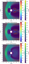 |
Fig. 1 Velocity fields (colored arrows, left colorbars) and plasma pressure (color contours, right colorbars) in the xz-plane for the open MS (θB = 0°, top), semi-open MS (θB = 90°, middle), and closed (θB = 180°, bottom) MS cases. Projected stellar wind magnetic field lines are indicated as solid black lines within the xz-plane parallel to the ambient magnetic field. Closed and open magnetospheric field lines are colored in magenta. |
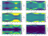 |
Fig. 2 Mercator projections of the Poynting flux (upper row), plasma velocity (middle row), and absolute values of Poynting flux components parallel to the unperturbed planetary field plus the small background field from stellar wind (bottom row). The results are shown at an altitude of one planetary radius above the surface. The left column displays maps for the open MS case (θB = 0°), the right column for the closed MS case (θB = 180°). Arrows indicate normalized angular components, and color contours denote radial components. Dashed red lines indicate the location of the OCFB. |
3.2 Poynting fluxes and aurorae
We are interested in understanding the electromagnetic coupling of the stellar wind with the MS of the exoplanet, its atmosphere and ionosphere. The energy fluxes associated with these electromagnetic coupling processes provide the energetics for the auroral emission from the exoplanet’s MS at radio and other wavelengths. Therefore, we study the Poynting flux to calculate the maximum available electromagnetic energy fluxes. We describe the spatial structure of magnetospheric Poynting fluxes in Sect. 3.2.1. Then we study the energetics of the interaction and effects of stellar wind variability on magnetospheric energetics in the subsequent Sects. 3.2.2 and 3.2.3.
3.2.1 Spatial structure
We first describe the spatial structure of the Poynting fluxes and plasma velocities within the MS as displayed in the top and middle row of Fig. 2, respectively. The plots show Mercator projections of the angular vector components over a spherical shell with radius 2 Rp. The figure shows the colatitude and longitude as well as the orientation of vectorial quantities and their magnitudes. Positive values indicate radial components pointing away from the planet. Also shown are the open-closed planetary field line boundaries (OCFBs). Magnetic field lines with both foot points on the planetary surface are closed field lines. Each field line that has only one foot point on the planet is an open field line. The OCFB separates areas with open from areas with closed field lines. Thus, the OCFB also represents the magnetopause at that specific radial location. Both open and closed MS cases are shown left and right, respectively.
The Poynting vector, S, can be rewritten in the ideal MHD case using the convective electrical field (e.g., Saur et al. 2013),
 (9)
(9)
which is bodily carried by the plasma flow perpendicular to magnetic field lines, denoted by the perpendicular velocity υ⊥. The Poynting flux describes the transport of magnetic enthalpy, which is a factor of two larger than the magnetic energy density, B2/2µ0 (e.g., Saur et al. 2013). In the remainder of this work, we mostly present Poynting fluxes, but need to consider the factor of two when we compare magnetic energy densities with thermal (i.e., internal energy) or kinetic energy densities based on their flows.
For both, the open and closed MS case, flow velocities are strongly reduced at the upstream (ϕ = 0–180 degrees) and downstream (ϕ = 180–360 degrees) side down to speeds below 10 km s−1. This occurs due to interaction with the intrinsic magnetic field and momentum transfer with the neutral atmosphere. The OCFB is located at roughly θ ≈ 30° and 150° in the open MS case. Due to the perfectly anti-parallel configuration of the stellar wind and planetary magnetic field no open planetary field lines exist in the closed MS model. This has also been observed in sub-Alfvénic simulations using this field topology (Ip et al. 2004; Strugarek et al. 2015).
Open magnetosphere model (Fig. 2 left)
The very narrow vertical extent of the downstream closed field line region of the open MS is caused by magnetic tension due to the magnetized stellar wind. Highest velocities are found within the open field line region mainly at the downstream side where plasma is accelerated downstream through magnetic tension on open lines.
Strong Poynting fluxes occur where plasma velocities have strong components perpendicular to the magnetic field. They are found within the open field line region mainly at the downstream side with outward directed Poynting fluxes. Comparatively strong Poynting fluxes, but directed toward the planet, are located on the upstream side near the magnetopause. Within the closed field line region and especially near the equator Poynting fluxes mostly vanish.
Closed magnetosphere model (Fig. 2 right)
In the closed MS model, highest velocities can be found near the planetary poles confined to an area below 25 degrees colatitude and similar in the south. These high velocities are caused by tension on high latitude closed field lines that are strongly stretched toward the downstream side by the stellar wind and reach up to 17 planetary radii. Poynting fluxes oriented away from the planet are confined to narrow bands encircling the high latitude polar regions between 40 and 80 degrees colatitude and similar in the south. At the upstream side Poynting fluxes vanish near the equatorial regions due to plasma flow being mainly aligned with planetary field lines. Inward oriented Poynting fluxes occur near the polar axis slightly shifted toward the downstream side.
We now study the Poynting fluxes parallel to the unperturbed background magnetic field because in the Solar System MSs they are considered the root energy fluxes from which a small fraction can be converted into auroral radio emission. Poynting fluxes provide the energy from which wave-particle interaction can draw energy to accelerate electrons (e.g., for Jupiter Hill 2001; Saur et al. 2021). The resulting energetic electrons then can be subject to the electron maser instability (Treumann 2006; Zarka 2007). The interaction of the stellar wind with τ Boötis b’s magnetic field perturbs the magnetic and electric field, which causes the Poynting fluxes. To quantitatively assess the associated Poynting flux, we therefore use the unperturbed magnetic background field B0 = Bp,0 + Bsw (i.e., the initial dipole and stellar wind field) to calculate the Poynting flux on this field,  . The unit vector
  points in the direction of unperturbed magnetic field lines. These projections give insight on where electromagnetic energy is transported through either propagating magnetic disturbances (i.e., Alfvén waves) or convection. The bottom row of Fig. 2 shows
  for the open MS (left) and closed MS (right). We note that only absolute values are shown in the plots in order to clearly identify zero or near-zero power densities.
Strongest energy transport along unperturbed field lines occurs over narrow bands encircling the polar open field line regions at the flanks of the planet where velocities are nearly perpendicular to the magnetic field as seen in Fig. 2. Moreover, the spatial structure of Poynting fluxes along B0 is strictly symmetric with respect to the equator (at θ = 90°). A significant amount of energy is transported parallel to the unperturbed field within the polar open field line regions in the open MS case. Parallel energy fluxes reach values up to 10 W m−2 at the flanks of the planet just outside the closed field line regions. Poynting fluxes up to 9 W m−2 are found at the downstream side, above the OCFB. For both, open and closed MS model, strongest convected energy can be found extensively in high latitude regions due to high velocities perpendicular to the magnetic field. Here the planetary field lines are most mobile in a sense that they are bent over toward the downstream side by the stellar wind. For the closed MS parallel Poynting fluxes up to roughly 9 W m−2 can be found directly at the planetary poles slightly shifted toward the upstream side. At lower latitudes parallel Poynting fluxes up to 6 W m−2 are confined to narrow bands at the flanks of the planet. Auroral emission is expected to be strong where Poynting fluxes are large, hence near the OCFB (e.g., mostly confined to the L = 3–3.5 shell at the upstream side) and in the polar regions for both MS models. They vanish completely along the equator. Generally said Poynting fluxes are significantly weaker and confined to the small polar regions for the closed MS model compared to the open MS case. In the open MS model strong parallel Poynting fluxes cover the whole open field line area with their maximum at the flanks of the planet in contrast to the closed MS where the regions of strongest parallel Poynting fluxes are partitioned into smaller areas around the planetary poles.
3.2.2 Energetics of the interaction
To estimate the total available Poynting flux, which serves as the root energy flux, we assume for simplicity that the radio emission is generated in a shell 1 Rp above the surface of the exoplanet. This particular choice is inspired by the fact that radio emission around Jupiter and other Solar System planets arises from altitudes about 1Rp (or larger) above the planet's surface (e.g., Zarka 1998; Hess & Zarka 2011) where strong electron acceleration takes place (e.g., for Jupiter Mauk et al. 2020). Poynting fluxes within the MS of τ Boötis b only vary little as a function of distance from the planet (see Appendix A for a discussion on the choice of r).
Available electromagnetic power for possible conversion into electron acceleration and radio emission is given by the divergence of the Poynting flux in this shell with volume V,
 (10)
(10)
where Ashell is the surface area of the shell and  the surface normal vector. To investigate the maximal Poynting flux that can be dissipated in the shell we assume that the Poynting flux entering the shell from above or below is dissipated within the shell. For mathematical simplicity, we further let the thickness of the shell grow infinitesimally small such that
 (11)
(11)
with Asphre the area of the sphere located at 2 RP from the center. In physical terms it means that the possible dissipation in the shell can be supplied with energy fluxes from below the shell (i.e., coming from the planet’s ionosphere) or from above the shell (i.e., coming from the MS or stellar wind). Ultimately, the energy flux is coming from the stellar wind, but the energy flux can be reflected or converted in the ionosphere and can be redirected away from the planet again. This integrated Poynting flux serves as a proxy for maximum available electromagnetic energy dissipated within an auroral acceleration region.
Alternatively, we integrate the components of the Poynting flux parallel to the unperturbed magnetic field, B0 = B – δB, where δB denotes the magnetic field perturbation generated by the interaction. These Poynting fluxes take into account the energy flux of which a fraction can directly contribute to particle acceleration and powering the ECMI-driven emission,
 (12)
(12)
where  is the unit vector pointing in direction of B0. We refer to this Poynting flux component as the auroral Poynting flux. As opposed to in Eq. (11), Pa, ‖ (Eq. (12)) serves as a more realistic estimator for calculating auroral energy dissipation since Eq. (11) includes a significant contribution of convected energy, which is likely not converted into particle acceleration. Table 2 summarizes integrated Poynting fluxes according to Eq. (11) (third column) for all three intrinsic magnetic field orientations. The 4th column shows integrated Poynting fluxes along the unperturbed field (Eq. (12)). Integrated Poynting fluxes range from 3.5 × 10¹⁸ down to 6.9 × 10¹⁷ W for the open toward the closed MS model. Poynting fluxes along the unperturbed field (Eq. (12)) amount to ~9 × 10¹⁷ and 1017 W for the open and closed MS, respectively. The effect of magnetic topology on convected energy within the MS is therefore significant as the powers differ by almost one order of magnitude. Magnetic stress due to the stellar wind interaction can work on the MSs less strongly if the MS is closed, thus giving rise to weaker flows and therefore weaker convected Poynting fluxes. The trend is similar for Poynting fluxes along B0, Pa, ‖, but here the powers are reduced by almost an order of magnitude below the integrated total Poynting fluxes Pa.
Integrated magnetospheric Poynting fluxes for different magnetic field topologies.
3.2.3 Influence of stellar wind variability on magnetospheric energetics
For modeling the space environment of τ Boötis b, the properties of its surrounding stellar wind carry very large uncertainties, in particular the stellar wind density. In Nicholson et al. (2016) and Vidotto et al. (2012), the coronal base density was estimated by choosing the electron density so that it can reproduce electron measure observations of τ Boötis A. The energy fluxes within the MS are powered by and limited by the maximum incident power of the stellar wind flow transferring onto the magnetospheric obstacle. Zarka (2007) found that the observed radio power of Solar System planets is nearly a constant fraction of the incident kinetic and magnetic energy convected through the obstacle's cross section,  , whereRmp is the magnetospheric stand-off distance of the magnetized planet. This energy is utilized in perturbing the topology of the planets magnetic field, which in turn results in currents induced by changes in magnetic flux. Therefore, the incident power controls the energetics within the MS. The magnetic Poynting flux, PB, and the kinetic energy flux, Pkin, convected through the obstacle's cross section can be calculated as follows:
 (13)
(13)
 (14)
(14)
Additionally, the thermal energy flux should be considered as well as it cannot be neglected for close-in orbits where stellar wind temperature, T, pressure and density are high,
 (15)
(15)
with nsw being the stellar wind particle density and υ0 denoting the incident stellar wind velocity.
The magnetopause distance Rmp can be obtained from an equilibrium between stellar wind and planetary ram  , magnetic (pB = B2/2µ0) and thermal pressure. Both, the magnetospheric thermal and ram pressures are considered negligible, thus pram,sw + pB, sw + ptherm, sw = pB, pl, where the subscript sw stands for stellar wind and pl for planet. The magnetopause distance (or magnetospheric stand-off distance) can then be calculated from
![Mathematical equation: ${R_{{\rm{mp}}}} = {R_{\rm{p}}}B_{\rm{p}}^{{1 \mathord{\left/ {\vphantom {1 3}} \right. \kern-\nulldelimiterspace} 3}}{\left[ {2{\mu _0}\left( {{1 \over 2}{\rho _{{\rm{sw}}}}\upsilon _0^2 + {p_{{\rm{sw}}}}} \right) + B_{{\rm{sw}}}^2} \right]^{{{ - 1} \mathord{\left/ {\vphantom {{ - 1} 6}} \right. \kern-\nulldelimiterspace} 6}}}.$](/articles/aa/full_html/2023/03/aa44947-22/aa44947-22-eq31.png) (16)
(16)
All parameters can be found in Table 1. The parameter υ0 refers to the relative velocity between the stellar wind and planet and Bp to the planetary surface magnetic field at the equator. A certain fraction of the total incident power,
 (17)
(17)
intersecting with the magnetopause can eventually be converted for the generation of radio emission within the MS. The fraction of total incident energy, ϵ, that may result in radio emission is expected to range from 10−5 to ~3 × 10⁻³ (i.e., Pradio = ϵPi) in the radiometric Bode law (see Fig. 3; Zarka 2007). We point out that various efficiencies for converting incident energy flux into electromagnetic radiation are discussed in the literature. For example, the efficiency of conversion from magnetospheric, auroral Poynting fluxes to radio emission, which accounts for the efficiency of electron acceleration through wave-particle interaction and the efficiency of the electron-cyclotron maser, should be separated from the generic efficiency factor obtained from the radiometric Bode law (Zarka 2007; see Fig. 3). For Jupiter’s radio emission the efficiency for conversion from magnetospheric, auroral Ponyting fluxes to radio emission is roughly 0.3–3 × 10⁻⁴ (Saur et al. 2021). We denote this efficiency by ϵa (Fig. 3).
As the stellar wind density is the most uncertain parameter we performed simulations with densities ranging from 0.05·ρ0 to 100·ρ0 (see Table 1 for the basic model). To get an understanding on how stellar wind variability affects the structure of the MS we show xz-plane slices similar to Fig. 1 for the two extreme cases (0.05·ρ0 and 100·ρ0) in Fig. C.1. We do not solve a self-consistent stellar wind model but instead follow the solar wind solution of Parker (1958) where the solution of the solar wind velocity υ(r) is independent of the coronal base density nc,0. In this solution, stellar mass and base temperature control υ(r) and T(r), where r is the distance from the Sun. For simplicity of the parameter study of this subsection, we chose an isothermal approach and changed the density together with the pressure, p0 (and therefore T), according to p0 ∝ ρ0 (see Eq. (15)). We therefore kept the temperature constant, and consequently, according to Parker (1958), the velocity does not change. Given the average stellar mass loss rate of τ Boötis A of Ṁ ≈ 2.3 × 10⁻¹² M⊙ yr−1 estimated by Nicholson et al. (2016) (see also our basic model, Table 1) the parameter range of stellar wind densities considered in this parameter study translates to mass loss rates between 1.15 × 10⁻¹³ M⊙ yr−1 and 2.3 × 10⁻¹⁰ M⊙ yr−1 since Ṁ ∝ρ0.
We integrated the Poynting flux along the unperturbed field over a spherical shell with radius 2Rp (e.g., Eq. (12)) in order to obtain an understanding of how much incident energy flux is eventually converted to auroral Poynting fluxes. Resulting powers are shown in Fig. 4 as a function of ρ0 (and ρ0). The simulated convected energy fluxes follow the trend of incident energy flux estimates (red solid line in Fig. 4) but are reduced to fractions of the total incident energy flux, Pi, between 15 and 20% for the open MS and between 1 and 5% for the closed MS. Changes to the stellar wind density ρ0 (and in the same manner p0) affect the incident power inflicted on  , but also influence the magnetospheric cross section in an opposite manner, as it can be seen in Fig. 4 (blue solid line). The magnetospheric stand-off distance scales according to
  and the incident energy flux with Pi ∝ ρsw + psw; therefore, the incident energy flux increase dominates over the effect of a shrinking MS due to increasing thermal and kinetic pressure. This is also validated by our simulation results (Fig. 4), implying an approximately linear scaling of auroral Poynting fluxes with ρ0 and p0 at least in the regime between 3 × 10¹¹ and 3 × 10¹³ H+ m−3. Below the point where stellar wind magnetic energy dominates over thermal and kinetic energy near 1011 H+ m−3, auroral Poynting fluxes seem to saturate near 2–3 × 10¹⁷ W (open MS) and near 1–2 × 10¹⁶ W (closed MS). Above 3 × 10¹³ H+ m−3 the increase of auroral Poynting fluxes with ρ0 (and p0) deviates further from the course of incident flux, implying a saturation toward 1019 W (open MS). This, however, has to be validated further through future simulations.
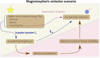 |
Fig. 3 Schematic illustrating the several steps from incident stellar wind energy flux toward auroral radio emission. The transfer function, Ta (see Sect. 4.1.1) describes the conversion from incident stellar energy to auroral Poynting fluxes. The conversion efficiency from auroral Poynting fluxes (Eq. (12)) to radio emission, ϵa, implicitly includes the efficiency of electron acceleration and the ECMI mechanism. The steps within the pink shaded area are not included in our model. Brown arrows indicate physical processes, blue arrows denote model parameters that quantify energy conversion, and the magenta arrow the radiometric scaling law. |
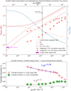 |
Fig. 4 Incident energy fluxes and auroral Poynting fluxes as a function of stellar wind density and pressure. Top: analytically calculated incident kinetic (dashed red line), Poynting (dotted red line), and thermal (dashed-dotted red line) energy fluxes convected through the magnetospheric cross section, |

4 Discussion
In this section, we discuss the importance of the stellar wind on magnetospheric energetics (Sect. 4.1) and on possible auroral radio emission (Sect. 4.2).
4.1 Impact of the stellar wind on magnetospheric energetics
In the following sections, we study the conversion of incident to dissipated power within the MS (Sect. 4.1.1) as a function of stellar wind density and pressure. We also discuss the limiting case of an absent stellar wind (Sect. 4.1.2).
4.1.1 Stellar wind variability, its effect on magnetospheric energetics, and the scaling behavior of auroral Poynting fluxes
We separate the considered stellar wind density and pressure range introduced in Sect. 3.2.3, Fig. 4 in two regimes: Regime 1 ranges from a vanishing stellar wind up to a density at roughly 1011 H+ m−3, where kinetic and thermal energy fluxes fall below the persistent magnetic energy flux, which dominates the flow (compare red curves in Fig. 4). Above roughly 1011 H+ m−3 the flow is super-Alfvénic (MA ≈ 2) and super-fast (Mf ≈ 1). The interaction is super-Alfvénic for the whole parameter space used in our simulations and sub-fast only for the lowest simulated density (ρsw = 7 × 10¹⁰ H+ m−3, MA ≈ 1.2). The incident energy nearly stagnates below ρ0 = 1010 H+ m−3 (red dotted line). Below this point the incident energy flux asymptotically approaches its minimum at 8 × 10¹⁷ W, as we assume that only the plasma density decrease but the incident magnetic field is kept constant. In this regime, it can be expected that the stellar wind magnetic field solution transitions from the Parker solution (e.g., B ∝ r−2) to a pure stellar multipole (here dipole) solution (e.g., Bsw = Bstar ∝ r−3) with decreasing stellar wind density. Eventually, when the stellar wind density hypothetically approaches zero, only the dipolar stellar magnetic field interacts with the planetary magnetic field. This limiting case will be separately discussed in Sect. 4.1.2.
Regime 2 ranges from roughly 1011 H+ m−3 up to arbitrarily high stellar wind densities. Here kinetic and thermal energy fluxes dominate the flow. We now focus on this regime. Considering the total energy flux convected through the magnetospheric cross section  , Ptotal (red solid line in Fig. 4), we observe a nearly constant efficiency of conversion from incident stellar wind energy toward magnetospheric Poynting fluxes at auroral altitudes (we assumed r ≈ 2Rp) with increasing density and pressure. We calculate the transfer function Ta as the conversion ratio from total incident energy flux Pi to the simulated auroral Poynting fluxes parallel to the unperturbed field (Eq. (12)), Pa (red crosses and stars in Fig. 4), within the MS, such that Ta = Pa/Pi (see Fig. 3 for a schematic illustrating the role of Ta). The transfer function also contains information on the magnetic topology and thus the efficiency of reconnection. The transfer function is displayed in the lower panel of Fig. 4. For the open MS, auroral Poynting fluxes decrease as a function of ρ0 and p0 according to an approximately constant ratio up to ~3 × 10¹³ H+ m−3. For higher densities and pressures, the transfer function scales with an exponent of ~−0.4, indicating a decrease of efficiency for conversion from incident to auroral energy fluxes. As the MS is increasingly compressed due to stronger ram and thermal pressures, the magnetopause eventually crosses the spherical shell with r = 2Rp after a critical density of ~3 × 10¹³ H+ m−3 and pressure of 3 × 10⁻⁴ Pa.
For the closed MS, Ta behaves differently. The transfer function instead increases slightly from 7 × 10¹⁰ to ~3 × 10¹³ H+ m−3 following a power law with exponent ~0.6. The opposite behavior compared to the open MS transfer function might be a consequence of a geometry where less reconnection occurs. The stronger ram and thermal pressure exert a stronger tension on planetary field lines, which in turn release stronger energy fluxes during reconnection.
4.1.2 Beyond the MHD limit
The more the stellar wind density decreases, the emptier the heliosphere of τ Boötis A becomes. In analogy with the solar wind, the stellar wind density upstream of the MS of τ Boötis b may change by orders of magnitude. The solar wind density is observed to vary by more than two orders of magnitude (see, e.g., Chané et al. 2012) such that Earth’s bow shock can disappear and the Earth develops Alfvén wings. In the hypothetical limit when the density approaches zero, τ Boötis b will still be exposed to the stellar magnetic field Bτ (r) (which then decreases according to Bτ(r) ∝ r−3 instead of Bsw ∝ r−2) and will propagate through it. Therefore, the incoming Poynting flux of the star does not, in contrast to kinetic and thermal energy flux, vanish and is maintained by the relative motion between the stellar and planetary magnetic field. In the case of an empty heliosphere, the interaction around τ Boötis b is no longer magnetohydrodynamic; it turns electromagnetic. Then the movement of τ Boötis b within the external magnetic field of the star is a unipolar or homopolar interaction (i.e., a moving conductive object with external field similar to a current generator in classical electromagnetism). In the case of a stellar magnetic field rotating at the same speed as the planet orbits around its host star (i.e., in the case of total orbital and spin synchronization), nonexistent changes in magnetic flux lead to a system where no work can be done by the magnetic fields. Therefore, no currents are induced and the MS remains energetically silent. Although it is expected that close-in exoplanets are in nearly tidally locked rotation, Murray & Dermott (2000) suggest in their textbook that completely synchronous rotation might not be possible if the planet has no permanent magnetic quadrupole moment and its eccentricity is not zero, which is the case for τ Boötis b (Wang & Ford 2011). Taking the rotation period of τ Boötis A, Pτ = 3.1 ± 0.1 days (Brown et al. 2021; Mengel et al. 2016), and the sidereal rotation period of τ Boötis b, Porb = 3.31 days (Butler et al. 1997; Wang & Ford 2011), we can calculate the relative velocity between the stellar and planetary magnetic field υ0 = 2πa × (1/Pτ − 1/Porb) ≈ 10.4 km s−1, where a = 0.046 AU is the semimajor axis of τ Boötis b. We use an average surface magnetic flux density of τ Boötis A obtained by Marsden et al. (2014); Mengel et al. (2016); Jeffers et al. (2018), Bτ, 0 = 2.4 G, and calculate the flux density at 0.046 AU using the dipole formula, Bτ(r = a) = Bτ, 0·(a/Rτ)−3 ≈ 0.73 G, where Rτ = 1.43 R⊙ is the stellar radius (Bonfanti et al. 2016). The magnetospheric stand-off distance in this case is defined purely by the balance of stellar and planetary magnetic pressure:
 (18)
(18)
Now we can calculate the stellar magnetic power convected on the MS using
 (19)
(19)
This value is included in Fig. 4 as magenta arrow. We can conclude the following: (a) The maximum possible magnetospheric stand-off distance is reached in complete absence of a stellar wind and if the stellar and planetary magnetic fields are antiparallel. If the stellar and planetary fields are parallel (i.e. open MS) the planetary field lines are all connected to the stellar field and no magnetopause can be determined. In the closed MS case the magnetopause lies at roughly 8.6 planetary radii in the upstream direction.
(b) Even if there is no stellar wind, the magnetic interaction between the stellar and planetary magnetic field still has the potential to drive an interaction with an available power limit of roughly 8 × 10¹⁵ W due to the relative motion of τ Boötis b in the stellar magnetic field. Radio emission would still be possible, although it would be very weak; corresponding radio fluxes at Earth’s position would be far below today’s telescope sensitivity limit. Considering Poynting flux-to-radio power efficiencies between 10−4 and 10−2, radio powers can reach values between 1011 and 1014 W. These emitted powers exceed the strongest radio sources within the Solar System by several orders of magnitude, with Jupiter’s aurora being the strongest radio emitter (Pradio ≈ 1010–1011 W, Zarka 2007), although Jupiter’s emission is, in contrast to close-in exoplanets, powered by internal, rotationally driven mechanisms. The transition from a MS interaction with a stellar wind field (according to the Parker solution, Parker 1958) to an interaction with a pure dipolar stellar magnetic field goes with an energetic transition followed by a decrease of maximum emitted radio power. This might pose a possible opportunity for constraining stellar wind densities in the future. Solving a self-consistent stellar wind model and comparing auroral Poynting fluxes for different stellar wind base densities could reveal the critical density range where the transition from a stellar magnetic-field-dominated electrodynamic interaction to a stellar-wind-dominated MHD interaction takes place. Comparing the magnetospheric Poynting fluxes and corresponding radio powers with possible future observations could reveal if the stellar wind density lies below or above the critical density.
4.2 Magnetospheric Poynting fluxes and auroral radio emission
In this section, we discuss possible radio emission scenarios (Sect. 4.2.1), study how magnetic topology of the interaction as well as stellar wind variability affects auroral radio emission output (Sect. 4.2.2). We also discuss the possibility of a sub-Alfvénic emission scenario (Sect. 4.2.3) as well as a rotation-driven MS of τ Boötis b in Sect. 4.2.4, followed by a discussion on possible source regions and radio frequencies of auroral emission in Sect. 4.2.5.
4.2.1 On the different radio emission scenarios
There are several scenarios capable of generating observable radio emission that must be distinguished from each other: (1) If the stellar wind is sub-Alfvénic, Alfvén waves are able to propagate upstream toward the stellar atmosphere along Alfvén wings and possibly drive electron acceleration and radio emission in the stellar vicinity. Local radio emission within the MS can also be generated in this scenario. We refer to this scenario as sub-Alfvénic emission scenario. This scenario is discussed briefly in Sect. 4.2.3.
(2) If the stellar wind is super-Alfvénic, no MHD wave is able to propagate upstream. The stellar wind-MS interaction, however, drives Poynting fluxes within the MS, which may, to some extent, generate auroral radio emission (see Fig. 3). We refer to this scenario as the magnetospheric emission scenario. Due to the stellar wind being super-Alfvénic for all simulations, we focus on the magnetospheric emission (Sect. 4.2.2).
(3) In a rotation-dominated MS scenario the rotating planet and its magnetic field causes corotation of magnetospheric plasma that, at some point, breaks down due to conservation of angular momentum if radial mass transfer takes place. This corotation breakdown exerts magnetic stresses on the field lines that are the root cause of auroral Poynting fluxes, which in turn drive auroral radio emission. This scenario is discussed in Sect. 4.2.4.
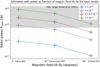 |
Fig. 5 Expected radio powers as a function of planetary magnetic axis tilt using auroral-to-radio power conversion efficiencies between 10−4 and 10−2. The auroral Poynting fluxes, S·B0, are integrated over a spherical shell with radius 2Rp. The gray shaded area represents the observational limits given by Turner et al. (2021). |
4.2.2 Effects of magnetic field tilt and stellar wind variability on auroral radio emission: Magnetospheric emission scenario
Figure 5 shows radio powers as a function of magnetic axis tilt. Radio powers are obtained by multiplying integrated auroral Poynting fluxes (i.e., Eq. (12)), which serve as a proxy for the maximum available electromagnetic energy that is transported along magnetic field lines, by efficiency factors for converting magnetospheric Poynting fluxes to radio power, ϵ, ranging from 10−4 to 10−2. This range covers proposed (Zarka 2007) and observed efficiency factors (e.g., ϵ ≈ 10−4 for Jupiter, Saur et al. 2021). The modeled magnetic field tilt can also be interpreted as stellar magnetic field orientation within this work, allowing us to study the effect of varying stellar magnetic field polarity on magnetospheric Poynting fluxes and limits for associated radio emission. Radio powers within the limits inferred from observations by Turner et al. (2021) lie within the gray shaded area. It is visible that efficiency factors in the range of ϵ ≈ (0.3 – 1) × 10−2 deliver radio powers most consistent with observations if the MS is open or at least semi open given the basic model (Table 1). This indicates that the efficiency of auroral Poynting fluxes driving electron acceleration and the electron cyclotron maser emission may be higher in the MS of τ Boötis b than in the Jovian MS (Saur et al. 2021). Electric fields generated by reconnection between stellar wind and planetary magnetic field lines are expected to contribute significantly to powering electron acceleration and therefore the ECMI (Jardine & Collier Cameron 2008). In our studies we find reconnection to indirectly play an important role (Fig. 5) because auroral Poynting fluxes and consequently radio powers drop by nearly an order of magnitude from an open to a closed MS. This is due to magnetic stress exerted by the stellar wind interaction being less strong for closed MSs. The polarity of τ Boötis A’s magnetic field switches every approximate 360 days (Fares et al. 2013). Shorter cycles in magnetic activity levels (by means of S-indices) were also observed (Mengel et al. 2016). A difference of half an order of magnitude to almost an order of magnitude can therefore be caused by a polarity reversal of τ Boötis A’s magnetic field. This results in radio emission whose observability is expected to fluctuate periodically in a nearly 1-year cycle. We note that the stellar wind magnetic field strength was kept constant in our parameter study, although in reality the field strength may vary strongly and influence produced radio emission significantly (See et al. 2015).
The emitted radio flux observed at Earth's position can be calculated with (Grießmeier et al. 2005, 2007b)
 (20)
(20)
where Ω is the solid angle of the beam and δv the emission bandwidth that is approximately equal to the maximum gyrofrequency (Grießmeier et al. 2007b), vg, e ≈ 24 MHz. We assume a solid angle of Ω = 1.6 sr, similar to Jupiter’s decametric radio emission (Zarka et al. 2004). The distance to the τ Boötis system is 15.6pc. We calculate the radio flux for both, the open and closed MS model, as a function of ρ0 and p0 with radio efficiencies ϵa = 10−4–10−2. The results are displayed in Fig. 6. Solid and dashed colored lines represent radio fluxes originating from open and closed MSs, respectively. The gray shaded area again denotes the range of observed radio fluxes form Turner et al. (2021). Horizontal gray lines indicate theoretical sensitivity limits of the LOFAR telescopes for 20 MHz. As stated by Turner et al. (2019), the realistic sensitivity might be slightly lower for circularly polarized (Stokes V) signals. We therefore include the expected sensitivity calculated by Turner et al. (2019) as yellow line. The results in Fig. 6 indicate that radio efficiencies between ~3 × 10⁻³ and ~10−2 are most consistent with the tentative observations (Turner et al. 2021). The efficiency account for several steps from conversion of auroral Poynting fluxes to radio emission (e.g., wave-particle interaction, electron acceleration and ECMI), and therefore an efficiency on the order of 1–10% might be unrealistic. The efficiency for Jupiter’s auroral emission is roughly ϵa = 0.3–3 × 10⁻⁴ (Saur et al. 2021), and therefore ϵa = 10−2 might be too high. Moreover, high plasma densities within the MS injected by the dense stellar wind and due to strong irradiation, which results in high ionization rates and inflated atmospheres (e.g., for v And b, see Erkaev et al 2022), may further decrease the ECMI efficiency or even prevent it (Weber et al. 2017, 2018; Daley-Yates & Stevens 2018) Assuming the radio efficiency to lie near 10−3, the radio flux from a closed MS falls below the detection threshold (yellow line). Therefore, in the case of a polarity reversal of τ Boöts A’s magnetic field (i.e., from aligned with the planetary field to anti-aligned), the radio signal would not be observable anymore in the case of radio efficiency equal or below ~3 × 10⁻³. In the case of ϵa ≈ 10−4 all radio fluxes for the basic model fall below the sensitivity limit. The observability increases, however, if stellar wind density and pressure rises, rendering ϵa = 10−3–10−2 to possible efficiencies to observe emission from open and closed MSs. Additionally, the ECMI efficiency (Treumann 2006; Weber et al. 2017) as well as efficiency of electron acceleration through wave-particle interaction decreases dramatically with increasing plasma density (Saur et al. 2018), making the higher density and pressure regime a less likely scenario to explain the tentative observations. As the pressure rises, the magnetopause is getting closer to the planet, reducing the space of magnetospheric diluted plasma regions between the magnetopause and atmosphere where radio emission might occur. We therefore conclude that the basic model (vertical gray line) and slightly different configurations represent the most likely scenarios if the emission is indeed generated by stellar wind-driven auroral Poynting fluxes. In this case radio emission is only observable, if the stellar wind and planetary magnetic fields are aligned (i.e., the MS is open). Given the high efficiencies (ϵ > 10−3) needed by ou model in order to generate radio emission that is consistent with the tentative observations, the magnetospheric emission scenario might not be energetic enough to explain the observations.
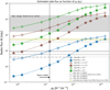 |
Fig. 6 Radio flux (Eq. (20)) as a function of stellar wind density and pressure for different efficiency factors. Colored solid and dashed lines represent fluxes for the open and closed MS models. Observational limits (Turner et al. 2021) are indicated by the gray shaded area. Horizontal gray lines display theoretical sensitivity limits of the LOFAR telescope. The real sensitivity for Stokes V signals obtained from Turner et al. (2019) is plotted as a yellow line. The vertical gray line marks the basic model (Table 1). |
4.2.3 Sub-Alfvénic emission scenario
Although there is no sub-Alfvénic interaction within the parameter space we considered, the possibility of such an interaction and its consequences on possible radio emission should not be neglected. By choosing a stellar wind density of psw = 0.03 ρ0 we find an Alfvénic Mach number of MA ≈ 0.9. In this case, Alfvén waves may propagate back to the star through Alfvén wings connecting the planetary magnetic field with the star. The electromagnetic energy channeled through this flux tube can be calculated using the model from Saur et al. (2013),
 (21)
(21)
where θ = 0° is the angle that describes the deviation of the flow from being perpendicular to the stellar wind magnetic field, Rmp ≈ 5 Rp the magnetospheric stand-of distance and  the interaction strength. Due to the planet presumably possessing an ionosphere, which favors a strong plasma interaction, we chose
  . Using υ0 and Bsw from our basic model (Table 1), the energy flux channeled through Alfvén wings parallel to magnetic field lines amounts to PS = 1.2 × 10¹⁸ W. This energy flux may contribute to electron acceleration and consequently to ECMI-driven radio emission in the space environment near the star. Taking the same range of Poynting flux to radio efficiencies (10−4–10−2), the expected radio power ranges from roughly 1014 to 1016 W, which partially overlaps with the range of radio power deduced by Turner et al. (2021). The emission frequency would, however, be much lower compared to the signals observed by Turner et al. (2021) due to the low magnetic field strength of τ Boötis A (Turner et al. 2021). Additionally, Turner et al. (2021) state that stellar emission would be less strongly circularly polarized compared to planetary emission. Nevertheless the root energy flux able to possibly drive radio emission near the stellar atmosphere from such a sub-Alfvénic interaction exceeds the auroral Poynting fluxes in the magnetospheric emission scenario by roughly half an order of magnitude. Consequently this scenario might provide energetically a possible explanation for the observed radio emission if the interaction is indeed sub-Alfvénic. This scenario requires the stellar wind density to be reduced by at least a factor of ~30 compared to our basic model. This, however, could well be within the realm of possible densities given the observed density variations of the solar wind even though the intervals of variability are short (Chané et al. 2012).
4.2.4 Rotationally dominated magnetospheric emission scenario
One of the possible generators for auroral emissions is radial mass transport within the MS as it is the case for Jupiter (e.g., Hill 2001; Zarka et al. 2018, Zarka et al. 2021). Plasma is moving radially outward due to centrifugal forces within an exoplanet’s MS. For small distances from the planet (or stellar host) the plasma corotates with the host. After a certain distance  in units of planetary radii,
  , the corotation breaks down due to conservation of angular momentum (i.e., the plasma orbits its host with a smaller angular velocity than those from the rotation of the host). The relative velocity exerts magnetic stresses on the frozen-in field lines, the tension accelerates plasma along the field lines back to the host. The distance of corotation breakdown can be estimated using the colatitude of the region, where auroral emission occurs, θa, following Hill (2001),
  . Saur et al. (2021) derived a so-called auroral power potential for magnetized rotation-dominated hosts,
 (22)
(22)
where the subscript host refers in our case to the planet τ Boötis b. The hosts magnetic flux density is denoted by Bhost, Ωhost ≈ 2π/Porb = 2.2 × 10⁻⁵ rad s−1 is its angular velocity and Rhost = Rp the planet’s radius. We note that the discussion in this subsection is only based on theoretical considerations since we neglected planetary rotation in our MHD model. Following Saur et al. (2021) we can calculate the energy flux due to mass transport, Pmag, by using
 (23)
(23)
where Σp denotes the Pedersen conductance. We assume a value of 1 S and 10 S that are of the same order of magnitude as observed conductances near Jupiter (e.g., Hill 2001; Strobel & Atreya 1983; Hinson et al. 1998). For a hot Jupiter exoplanet the ionospheric Pedersen conductivity might be larger due to the larger ionization (Koskinen et al. 2010). However, the height of the resulting ionospheric layer and thus the mobility of the electrons and ions within the atmosphere also play an important role for the values of its conductivity. To our knowledge no dedicated study for the conductance of τ Boötis b is available. We also note that in Eq. (22) the distance of corotation breakdown  is proportional to Σ1/4 (Hill 2001). Thus, the Pmag in Eq. (23) depends effectively weaker on Σp (i.e., Pmag is proportional to
  ). In our simulations we integrate the ion component of the Pedersen conductivity along the z-axis at the poles from the surface (r = Rp) to r = 1.1 Rp where the plasma density peaks and find the height integrated Pedersen conductance to be on the order of 10 S. We find, with aurora occurring at field lines with L-parameter smaller than ~4 that have to lie within the MS (e.g.,
  ), the auroral power potential to be Spot ≈ 0.5 W m−2 S−1 and the magnetic power to lie between Pmag ≈ 1014 W and 1015 W. The auroral power potential of Jupiter, for comparison, is roughly 600 W m−2 S−1. The resulting energy flux between the MS and ionosphere lies near the Jovian value (3.1 × 10¹⁴ W, Saur et al. 2021). This result is several orders of magnitude below the power of magnetospheric Poynting fluxes powered by the stellar wind-planet interaction in our model (e.g., 1017–1018 W, Table. 2). Therefore, we can safely assume that the MS of τ Boötis b is not rotationally dominated, which is in agreement with the expected slow rotation nearly synchronized with its orbit around the star.
4.2.5 Properties and source regions of possible auroral radio emission
Auroral radio emission is mainly characterized by signal strength and frequency. The peak frequency is defined by the local electron gyrofrequency,
 (24)
(24)
where e is the electron charge, me its mass and B the local magnetic flux density (Farrell et al. 1999; Grießmeier et al. 2007a,b). We already discussed possible radio powers from τ Boötis b in Sects. 3.2.2 and 4.2.2, now we focus on possible signal frequencies. Turner et al. (2021) observed signals within the 21–30 MHz range. The magnetic flux density inferred from the maximal signal frequency by the authors is almost certainly underestimated since ECMI-driven auroral radio emission typically arises from altitudes above the polar regions of the planet’s atmosphere (Zarka 1998; Hess & Zarka 2011) due to three reasons: (a) High ionospheric electron densities cause the electron plasma frequency, νp, e, to exceed the local gyrofrequency, νp, e, thus prohibiting the transmission of emitted waves; (b) radio wave amplification through the ECMI mechanism works most efficiently in regions where νg, e >> νp, e (Treumann 2006; Weber et al. 2017) and (c) the electrons are usually accelerated in regions where the plasma density along a field line is the smallest (or B/n is maximum; e.g., Saur et al. 2018). There wave particle interaction to accelerate electrons is maximum efficient.
The electron plasma frequency is given by
 (25)
(25)
where ne = ni is the particle density in a quasi-neutral plasma and ϵ0 the vacuum permittivity. The source regions of Jupiter’s radio emission lie several planetary radii above the surface (e.g., Zarka 1998) where strongest electron acceleration is expected (e.g., Mauk et al. 2017). The maximum gyrofrequency in our model (directly above the magnetic poles) is ~24 MHz. Auroral emission, however, typically arises from near the OCFB. In our simulations we indeed see that strongest Poynting fluxes are confined to narrow bands encircling the OCFB (or magnetopause) near L = 3 and L = 3.5 shell field lines (Fig. 2). Since source regions of ECMI induced emission typically lie at higher altitudes the magnetic flux density and thus emission frequency is even further reduced. The conditions (a–c) for efficient ECMI-driven radio emission might particularly be fulfilled for regions with low plasma density at the night side of the planet where the shadow exerted by the planet prevents photoionization. Since τ Boötis b is likely in tidally locked rotation around its host star, the night side might exhibit relatively low temperatures, favoring a recombination of electrons and hydrogen ions as well as further electron capture processes. In the shadow zone (i.e., permanent night side of the planet), ECMI induced emission might be more likely and might as well occur in lower altitudes, where the magnetic field is stronger (and thus emission frequency is higher).
5 Conclusions
In this study, we have modeled the MS of the hot Jupiter exoplanet τ Boötis b and its interaction with the stellar wind. In order to study magnetospheric energetics by means of Poynting fluxes, we performed MHD simulations of the near space environment of τ Boötis b with the stellar wind being injected into the simulation domain. The magnetic field of τ Boötis b was constrained by tentative observations of auroral radio emission (Turner et al. 2021). The stellar wind model is based on simulations where observed magnetic surface maps of τ Boötis A were utilized (Nicholson et al. 2016; Vidotto et al. 2012). We investigated magnetospheric energetics, available electromagnetic power, and limits of possible radio emission originating from above the planet's polar regions. We also explored the possibility of a rotation-dominated magnetospheric emission scenario as well as a sub-Alfvénic (stellar) emission scenario. The effect of stellar wind variability in terms of density, pressure, and magnetic field orientation on magnetospheric energetics was additionally investigated.
We find that the stellar wind-MS interaction is super-fast and super-Alfvénic for the majority of stellar wind densities and pressures considered in this study (from 1.4 × 10¹¹ H+ m−−3 and 2.5 × 10⁻⁶ Pa to arbitrarily high stellar wind densities and pressures). For the minimum density and pressure considered in this work (ρsw = 7 × 10¹⁰ H+ m−3 and psw = 1.3 × 10⁻⁵ Pa), the interaction is super-Alfvénic and sub-fast. Maximum available electromagnetic energy convected within the MS amounts to 3.5 × 10¹⁸ W, 1.8 × 10¹⁸ W, and 7 × 10¹⁷ W for an open, semi-open, and closed MS configuration. Auroral Poynting fluxes at altitudes of 1Rp above the planet reach powers of 8.7 × 10¹⁷ W down to 1.1 × 10¹⁷ W for the open and closed MS, indicating a strong decrease in stellar wind energy converted to auroral Poynting fluxes as a function of magnetic field tilt (either stellar or planetary).
We present Poynting flux maps of the planet’s near space environment. The strongest Poynting fluxes are confined to narrow bands encircling the OCFBs (i.e., the magnetopause) that are displaced toward the planet’s downstream side due to magnetic stresses exerted by the stellar wind and its high plasma β. Electromagnetic energy transported parallel to unperturbed field lines is also confined to bands near the magnetopause and the polar open-field-line regions.
Considering the stellar wind density as a free parameter, we chose values between 0.05 and 100 times the basic density, ρsw = 1.4 × 10¹² H+ m−3 (Table 1), and changed the stellar wind pressure in the same manner in order to keep the wind isothermal. Comparing the incident total energy flux convected through the magnetospheric cross section, we find that the transfer function, Ta (i.e., the amount of stellar wind incident energy flux converted to magnetospheric Poynting fluxes parallel to unperturbed field lines) amounts to a fraction of roughly 20 % for the open and 2 % for the closed MS. We find that  and
and  for the open and closed MS, respectively, in the density range 7 × 10¹¹–2×10¹³ H+ m−3. Increasing the stellar wind ram and thermal pressure and thus the incident energy flux causes the MS to shrink. The reduced capability of the MS for receiving stellar wind energy is outperformed by the increasing pressure and density. The scaling of Ta and thus the energy output of the MS nearly stagnates from that point on: the magnetopause becomes so small that the planetary atmosphere starts to interact with the pre-bow-shock and magnetosheath flow.
We investigated different radio emission scenarios. A rotation-dominated magnetospheric emission scenario can be ruled out due to the expected long rotation period of τ Boötis b. The estimated magnetic power generated by the planet's rotation is on the order of Pmag ≈ 1014–15 W. As this would require a very high Poynting flux-to-radio efficiency of 10−2, we expect that this scenario is not powerful enough to drive the tentatively observed radio emission.
We considered several efficiencies for the conversion of auroral Poynting fluxes to radio emission and compared the results with observations together with theoretical limits based on the tentative observations by Turner et al. (2021). We find that the generation of radio emission near τ Boötis b requires relatively high efficiencies (ϵa ≈ 1–5 × 10⁻³) compared to estimates from Jupiter’s rotationally driven aurora (up to ~3 × 10⁻⁴; Saur et al. 2021) in order to explain the observed emission if we assume the emission to originate from the MS of τ Boötis b. Furthermore, we find a strong dependence of radio emission observability on MS topology. In the case of a polarity reversal of τ Boötis A’s magnetic field from an aligned to anti-aligned configuration (with respect to the planetary field), the estimated radio power falls below the observational limit. We therefore expect an on-off nature of detectable radio emission in phase with τ Boötis A’s magnetic cycle.
We also considered the case of a sub-Alfvénic interaction, which requires the stellar wind density to be at least a factor of 30 lower compared to our basic model. The Poynting flux channeled toward the host star due to this interaction amounts to ~1018 W, which slightly exceeds the power converted by the magnetospheric emission scenario.
Acknowledgements
This project has received funding from the European Research Council (ERC) under the European Union's Horizon 2020 research and innovation programme (grant agreement No. 884711). We furthermore thank the Regional Computing Center of the University of Cologne (RRZK) for providing computing time on the DFG-funded (Funding number: INST 216/512/1FUGG) High Performance Computing (HPC) system CHEOPS as well as support. We also thank Stefan Duling for providing several basic model implementations for the Pluto code used in this study as well as for helpful discussions.
Appendix A Poynting fluxes as a function of radial distance from the planet
Here we study the dependence of magnetospheric Poynting fluxes as a function of radial distance from the planet. The particular choice of integrating Poynting fluxes over a spherical shell with radius r = 2Rp is based on the fact that radio emission around Jupiter and most Solar System planets with intrinsic magnetic fields originates from altitudes of about 1 Rp or higher above the planets (see, e.g., Zarka 1998) rather than from within the ionosphere or even further below. We do not have evidence as to whether this translates to extrasolar planets but simply assume so. For the ECMI mechanism to work efficiently the ratio between electron gyrofrequency and plasma frequency, νg, e/νp, e, must be significantly larger than 1, which turns the magnetospheric region at high altitudes to favored radio source regions where plasma densities are strongly reduced compared to other regions of the MS. (Zarka 1998; Treumann 2006; Weber et al. 2017). Considering the plasma and neutral particle density within the modeled MS we also chose a location (i.e., the radius) where ion-neutral collisions are significantly reduced (e.g., above the ionosphere). The favored radius according to this constraint lies between 1.3 and 3 Rp (see Sect. D and Fig. D.2).
In order to show that the choice of r = 2 Rp or any other radial distance within the MS does not influence the results and the derived conclusions significantly (despite controlling the emission frequency since stronger magnetic fields cause higher gyro frequencies) we integrated the Poynting flux (Eq. 11) for shells with radii between 1 and 2.5 Rp above the planet. The results are displayed in Fig. A.1 for the open (blue), semi-open (orange) and closed (green) MS model. We note that the Poynting flux is not a conserved quantity in this system since several possibilities for conversion from or to electromagnetic energy exist within the MS (e.g., deceleration due to magnetic stresses, ion-neutral collisions, conversion between electromagnetic and thermal energy). As it can be seen in Fig. A.1 the Poynting flux variation as a function of r amounts to a factor of ~ 1.5–2 for the open MS, ~ 1–1.5 for the semi-open MS and ~2 for the closed MS. Given the uncertainties with which our study is anyway afflicted (such as the uncertainty of the stellar wind density, magnetic field strength, etc.), the uncertainty by the choice of the shell radius upon the Poynting fluxes is negligible. The choice of magnetic field strength, for instance, has much larger influence on the Poynting fluxes due to its B2 dependence.
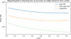 |
Fig. A.1 Magnetospheric Poynting flux as a function of radial distance from the planet’s center, calculated from Eq. 11, for the open (blue), semi-open (orange), and closed (green) MS models. |
Appendix B On the effect of magnetic diffusion on the results
In our MHD model we include the ionosphere and atmosphere of τ Boötis b through collisions with the plasma. We do not include the effects of collisions in the induction equation for computational time reasons. In this section we justify this simplification by comparing simulations with different physical diffusion rates (i.e., different ionospheric conductivities) compared to our basic model without diffusion.
Therefore, we add a diffusion term to the induction equation (Eq. 4), which then reads
![Mathematical equation: ${{\partial {\bf{B}}} \over {\partial t}} = \nabla \times \left[ {{\bf{\upsilon }} \times {\bf{B}} - \eta \nabla \times {\bf{B}}} \right].$](/articles/aa/full_html/2023/03/aa44947-22/aa44947-22-eq55.png) (B.1)
(B.1)
We scaled the magnetic diffusivity η = η(r) with the atmospheric scale height so that it correlates with the neutral particle density,
 (B.2)
(B.2)
where η0 is the surface magnetic diffusivity, Rp = 72875 km the planetary radius (Wang & Ford 2011), r the radial distance from the planet center and H = 4373 km the scale height (see Table 1 and Sect. 2.3).
We assumed a range of height integrated Pedersen conductivities, ΣP, between 1 and 100 S. Together with the scale height we can calculate the surface magnetic diffusivity with
 (B.3)
(B.3)
where µ0 is the vacuum permeability. The expected range of surface diffusivities is therefore  and
and  for conductances of 100 S and 1 S, respectively.
In order to study the effect of magnetic diffusion on our simulation results, we compare the simulated plasma variables B, p, ρ and υ within the MS of τ Boötis b with and without magnetic diffusion near the planet at r = 2 Rp. We restrict ourselves to simulations with open MSs using the basic stellar wind model.
The deviations of the four plasma variables simulated with diffusion from those simulated without are displayed in Figs. B.1 ( , ΣP = 100 S) and B.2 (
 , ΣP = 1 S) given in arbitrary normalized units. The finite conductivity causes only very small deviations from our basic model at r = 2Rp on the order of 10−3 for a diffusive model with 1 S Pedersen conductance. Maximum deviations at r = 2Rp for the diffusive model with ΣP = 100 S amount to factor of 10−5 (Fig. B.1) compared with the non-diffusive model.
We thus conclude that the effect of magnetic diffusion on our results (i.e., the magnetospheric Poynting flux) at 2 Rp above the ionosphere of the planet is negligible.
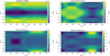 |
Fig. B.1 Deviations of resistive MHD simulations from the simulations discussed in the main text using the basic model (Table 1). The results correspond to simulations with a Pedersen conductance of 100S. The four panels display magnetic field (upper left), pressure (upper right), density (bottom left), and velocity (bottom right) maps at r = 2Rp. |
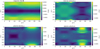 |
Fig. B.2 Deviations of resistive MHD simulations from the simulations discussed in the main text using the basic model (Table 1). The results correspond to simulations with a Pedersen conductance of 1S. The four panels display magnetic field (upper left), pressure (upper right), density (bottom left), and velocity (bottom right) maps at r = 2Rp. |
Appendix C Structure of the interactions: Parameter study
In order to illustrate the effect of stellar wind density and pressure on the magnetospheric structure, we show xz-plane slices (Figs. C.1) similar to Fig. 1 for the extreme cases (0.05 ρsw and 100 ρsw) of our parameter study (Sects. 3.2.3 and 4.1.1). The plots show plasma velocity and thermal pressure in the near space environment of τ Boötis b. We use spherical coordinates to numerically describe the space environment around τ Boötis b. These coordinates have mathematical singularities along the pole axis. For exceptionally small upstream plasma densities, this can lead to numerical artifacts (i.e., jumps for the scalar variables along the pole axis in the PLUTO code). This is visible in Fig. C.1 (left). In the vector fields and thus the Poynting fluxes this discontinuity is negligible. This effect occurring at the extremely low upstream conditions thus does not have an effect on the conclusions of this work.
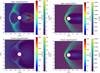 |
Fig. C.1 Plasma interaction for density ρsw = 0.05 ρ0 (left panels) and density ρsw = 100 ρ0 (right panels). Displayed are velocity fields (colored arrows, left colorbars) and plasma pressure (color contours, right colorbars) in the xz-plane for the open MS (θB = 0°, top) and closed MS cases (θB = 180°, bottom). Closed and open magnetospheric field lines are colored in magenta. |
The effect of stellar wind pressure and density on the size of the MS is clearly visible. The day side magnetopause location is ~5 Rp for the lowest density case (0.05 ρsw, left panels) and ~1.2Rp for the highest density case (100 ρsw, right panels). Also visible is the sub-fast nature of the interaction in the lowest density case, where no bow shock forms upstream and thus incident plasma flow is perturbed prior to intersecting with the MS.
Appendix D On the neutral atmosphere model assumptions and its interaction with the plasma
In this section we discuss some properties and assumptions on our neutral atmosphere model presented in Sect. 2.3 as well as how the atmosphere affects the plasma focusing on our basic model (Table 1).
The aim of this work is not a detailed description of the ionosphere of the planet, but rather its MS and larger space environment. Our simplistic atmosphere model only acts through collisions with the plasma and affects the photoionization rate (i.e., plasma production). These processes directly scale with the neutral particle density (Eqs. 5, 6). Due to the exponential decrease of neutral particle density (Eq. 5) with radial distance from the planet the atmosphere's effect on the plasma population drastically decreases with increasing altitude. The denser the neutral atmosphere, the more the magnetospheric plasma is decelerated; this leads to plasma piling up around the planet, mimicking an ionosphere. Figure D.2 shows plasma density profiles within the MS as a function of radial distance from the center. The black dotted line represents the plasma density along the polar axes. Red and magenta lines represent equatorial upstream and downstream profiles, respectively. The orange solid line denotes the neutral particle density according to Eq. 5, the green dotted line shows the corresponding ion-neutral collision frequency. As visible in Fig. D.2 the effect of ion-neutral collisions and thus the amount of plasma pile up is drastically reduced above an altitude near 1.3 Rp. There the neutral particle density is n(r = 1.3Rp) ≈ 5 × 10¹⁰ m−3. The ion-neutral collision frequency is ~0.5 s−1 at the surface and drastically decreases with altitude. In our studies we focus on the region 1 Rp above the planets surface and thus above the ionospheric shell. At r = 2 Rp the collisions are negligible because the collision frequency has decreased to about ~10−7 s−1.
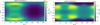 |
Fig. D.1 Plasma density maps over a sphere with r = 2Rp for the open (left panel) and closed MS cases (right panel). |
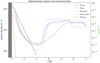 |
Fig. D.2 Plasma density profiles along the polar axis (dotted black line), upstream (red), and downstream x-axis (magenta). The solid blue line denotes the mean plasma density profile. The solid orange line shows the neutral particle density according to our atmosphere model (Eq. 5). The solid green line (right y-axis) denotes ion-neutral collision frequencies. |
The large scale height of 4373 km increases the extent of the atmosphere but is needed in order to sufficiently resolve the atmosphere in our model. However, the atmospheres of hot Jupiter exoplanets are expected to be strongly inflated due to intense stellar irradiation (e.g., Vidal-Madjar et al. 2003), which is partially mimicked by the large scale height. The surface neutral particle density n0 corresponds to an atmosphere pressure near 10−3 nbar assuming a temperature between 1000 and 2000 K. Here the mixing ratio of plasma (hydrogen ions) and neutral particles is roughly 50 %. The neutral atmosphere consists of molecular hydrogen, which is the most abundant molecule in all Solar System gas giants.
In order to demonstrate the minor role of the neutral atmosphere at r = 2 Rp we show plasma density maps over a shell at this altitude in Fig. D.1. The left and right panels display the density map of the open and closed MS case, respectively. There the neutral particle density is n(r = 2 Rp) ≈ 4.6 × 10⁵ m−3 according to Eq. 5 and Fig. D.2, leading to a neutral-plasma mixing ratio of about 10−6. Regions of high plasma density (i.e., at the day side) indicate regions where the interaction between the neutral atmosphere and plasma is strongest (at r = 2 Rp) in terms of ionneutral collisions and recombination. However, the effect of the neutral atmosphere on the plasma is an order of magnitude lower than in regions within the ionosphere below ~1.3 Rp.
References
- Alexander, R.D., Wynn, G.A., Mohammed, H., Nichols, J.D., & Ercolano, B. 2016, MNRAS, 456, 2766 [CrossRef] [Google Scholar]
- Atreya, S.K., Mahaffy, P.R., Niemann, H.B., Wong, M.H., & Owen, T.C. 2003, Planet. Space Sci., 51, 105 [NASA ADS] [CrossRef] [Google Scholar]
- Bastian, T., Cotton, B., & Hallinan, G. 2022, ApJ, 935, 99 [NASA ADS] [CrossRef] [Google Scholar]
- Bisikalo, D.V., Kaigorodov, P.V., Ionov, D.E., & Shematovich, V.I. 2013, Astron. Rep., 57, 715 [NASA ADS] [CrossRef] [Google Scholar]
- Bonfanti, A., Ortolani, S., & Nascimbeni, V. 2016, A&A, 585, A5 [NASA ADS] [CrossRef] [EDP Sciences] [Google Scholar]
- Brown, E.L., Marsden, S.C., Mengel, M.W., et al. 2021, MNRAS, 501, 3981 [NASA ADS] [CrossRef] [Google Scholar]
- Butler, R.P., Marcy, G.W., Williams, E., Hauser, H., & Shirts, P. 1997, ApJ, 474, L115 [NASA ADS] [CrossRef] [Google Scholar]
- Cauley, P.W., Shkolnik, E.L., Llama, J., & Lanza, A.F. 2019, Nat. Astron., 3, 1128 [NASA ADS] [CrossRef] [Google Scholar]
- Chané, E., Saur, J., Neubauer, F.M., Raeder, J., & Poedts, S. 2012, J. Geophys. Res. Space Phys., 117, A09217 [Google Scholar]
- Cohen, O., Kashyap, V.L., Drake, J.J., et al. 2011, ApJ, 733, 67 [NASA ADS] [CrossRef] [Google Scholar]
- Cohen, O., Drake, J.J., Glocer, A., et al. 2014, ApJ, 790, 57 [NASA ADS] [CrossRef] [Google Scholar]
- Cohen, O., Moschou, S.-P., Glocer, A., et al. 2018, AJ, 156, 202 [NASA ADS] [CrossRef] [Google Scholar]
- Cuntz, M., Saar, S.H., & Musielak, Z.E. 2000, ApJ, 533, L151 [NASA ADS] [CrossRef] [Google Scholar]
- Daley-Yates, S., & Stevens, I.R. 2018, MNRAS, 479, 1194 [NASA ADS] [Google Scholar]
- Dedner, A., Kemm, F., Kröner, D., et al. 2002, J. Comput. Phys., 175, 645 [Google Scholar]
- Donati, J.F., Moutou, C., Farès, R., et al. 2008, MNRAS, 385, 1179 [CrossRef] [Google Scholar]
- Duling, S., Saur, J., & Wicht, J. 2014, J. Geophys. Res. Space Phys., 119, 4412 [NASA ADS] [CrossRef] [Google Scholar]
- Erkaev, N.V., Weber, C., Grießmeier, J.M., et al. 2022, MNRAS, 512, 4869 [NASA ADS] [CrossRef] [Google Scholar]
- Fares, R., Donati, J.F., Moutou, C., et al. 2009, MNRAS, 398, 1383 [NASA ADS] [CrossRef] [Google Scholar]
- Fares, R., Moutou, C., Donati, J.F., et al. 2013, MNRAS, 435, 1451 [NASA ADS] [CrossRef] [Google Scholar]
- Farrell, W.M., Desch, M.D., & Zarka, P. 1999, J. Geophys. Res., 104, 14025 [NASA ADS] [CrossRef] [Google Scholar]
- Franklin, K.L., & Burke, B.F. 1958, J. Geophys. Res., 63, 807 [NASA ADS] [CrossRef] [Google Scholar]
- Gray, R.O., Napier, M.G., & Winkler, L.I. 2001, AJ, 121, 2148 [NASA ADS] [CrossRef] [Google Scholar]
- Griessmeier, J.M. 2017, in Planetary Radio Emissions VIII, eds. G. Fischer, G. Mann, M. Panchenko, & P. Zarka, 285 [Google Scholar]
- Grießmeier, J.-M. 2015, in Characterizing Stellar and Exoplanetary Environments, eds. H. Lammer, & M. Khodachenko, Astrophysics and Space Science Library, 411, 213 [CrossRef] [Google Scholar]
- Grießmeier, J.M., Motschmann, U., Mann, G., & Rucker, H.O. 2005, A&A, 437, 717 [NASA ADS] [CrossRef] [EDP Sciences] [Google Scholar]
- Grießmeier, J.M., Preusse, S., Khodachenko, M., et al. 2007a, Planet. Space Sci., 55, 618 [CrossRef] [Google Scholar]
- Grießmeier, J.M., Zarka, P., & Spreeuw, H. 2007b, A&A, 475, 359 [NASA ADS] [CrossRef] [EDP Sciences] [Google Scholar]
- Grießmeier, J.M., Zarka, P., & Girard, J.N. 2011, Radio Sci., 46, RS0F09 [Google Scholar]
- Gurumath, S.R., Hiremath, K.M., & Ramasubramanian, V. 2018, IAU Sympos., 340, 242 [CrossRef] [Google Scholar]
- Hess, S.L.G., & Zarka, P. 2011, A&A, 531, A29 [NASA ADS] [CrossRef] [EDP Sciences] [Google Scholar]
- Hill, T.W. 2001, J. Geophys. Res., 106, 8101 [NASA ADS] [CrossRef] [Google Scholar]
- Hinson, D.P., Twicken, J.D., & Karayel, E.T. 1998, J. Geophys. Res., 103, 9505 [NASA ADS] [CrossRef] [Google Scholar]
- Ip, W.-H., Kopp, A., & Hu, J.-H. 2004, ApJ, 602, L53 [NASA ADS] [CrossRef] [Google Scholar]
- Jardine, M., & Collier Cameron, A. 2008, A&A, 490, 843 [NASA ADS] [CrossRef] [EDP Sciences] [Google Scholar]
- Jeffers, S.V., Mengel, M., Moutou, C., et al. 2018, MNRAS, 479, 5266 [NASA ADS] [CrossRef] [Google Scholar]
- Kavanagh, R.D., Vidotto, A.A.Ó., Fionnagáin, D., et al. 2020, in Solar and Stellar Magnetic Fields: Origins and Manifestations, eds. A. Kosovichev, S. Strassmeier, & M. Jardine, 354, 305 [NASA ADS] [Google Scholar]
- Kavanagh, R.D., Vidotto, A.A., Klein, B., et al. 2021, MNRAS, 504, 1511 [NASA ADS] [CrossRef] [Google Scholar]
- Kavanagh, R.D., Vidotto, A.A., Vedantham, H.K., et al. 2022, MNRAS, 514, 675 [CrossRef] [Google Scholar]
- Kislyakova, K.G., Holmström, M., Lammer, H., Odert, P., & Khodachenko, M.L. 2014, Science, 346, 981 [NASA ADS] [CrossRef] [Google Scholar]
- Kislyakova, K.G., Pilat-Lohinger, E., Funk, B., et al. 2016, MNRAS, 461, 988 [NASA ADS] [CrossRef] [Google Scholar]
- Kopp, A., Schilp, S., & Preusse, S. 2011, ApJ, 729, 116 [NASA ADS] [CrossRef] [Google Scholar]
- Koskinen, T.T., Cho, J.Y.K., Achilleos, N., & Aylward, A.D. 2010, ApJ, 722, 178 [NASA ADS] [CrossRef] [Google Scholar]
- Lai, D., Helling, C., & van den Heuvel, E.P.J. 2010, ApJ, 721, 923 [NASA ADS] [CrossRef] [Google Scholar]
- Llama, J., Wood, K., Jardine, M., et al. 2011, MNRAS, 416, L41 [NASA ADS] [CrossRef] [Google Scholar]
- Maggio, A., Sanz-Forcada, J., & Scelsi, L. 2011, A&A, 527, A144 [NASA ADS] [CrossRef] [EDP Sciences] [Google Scholar]
- Marsden, S.C., Petit, P., Jeffers, S.V., et al. 2014, MNRAS, 444, 3517 [NASA ADS] [CrossRef] [Google Scholar]
- Mauk, B.H., Haggerty, D.K., Paranicas, C., et al. 2017, Geophys. Res. Lett., 44, 4410 [CrossRef] [Google Scholar]
- Mauk, B.H., Clark, G., Gladstone, G.R., et al. 2020, J. Geophys. Res. Space Phys., 125, e27699 [NASA ADS] [Google Scholar]
- Mengel, M.W., Fares, R., Marsden, S.C., et al. 2016, MNRAS, 459, 4325 [NASA ADS] [CrossRef] [Google Scholar]
- Mignone, A., Bodo, G., Massaglia, S., et al. 2007, in JENAM-2007, “Our NonStable Universe”, 96 [Google Scholar]
- Mignone, A., Tzeferacos, P., & Bodo, G. 2010, J. Comput. Phys., 229, 5896 [Google Scholar]
- Miller, B.P., Gallo, E., Wright, J.T., & Dupree, A.K. 2012, ApJ, 754, 137 [NASA ADS] [CrossRef] [Google Scholar]
- Miller, B.P., Gallo, E., Wright, J.T., & Pearson, E.G. 2015, ApJ, 799, 163 [NASA ADS] [CrossRef] [Google Scholar]
- Mittag, M., Robrade, J., Schmitt, J.H.M.M., et al. 2017, A&A, 600, A119 [NASA ADS] [CrossRef] [EDP Sciences] [Google Scholar]
- Murray, C.D., & Dermott, S.F. 2000, Solar System Dynamics (Cambridge University Press) [CrossRef] [Google Scholar]
- Nichols, J.D., & Milan, S.E. 2016, MNRAS, 461, 2353 [NASA ADS] [CrossRef] [Google Scholar]
- Nicholson, B.A., Vidotto, A.A., Mengel, M., et al. 2016, MNRAS, 459, 1907 [CrossRef] [Google Scholar]
- Parker, E.N. 1958, ApJ, 128, 664 [NASA ADS] [CrossRef] [Google Scholar]
- Preusse, S., Kopp, A., Büchner, J., & Motschmann, U. 2006, A&A, 460, 317 [NASA ADS] [CrossRef] [EDP Sciences] [Google Scholar]
- Preusse, S., Kopp, A., Büchner, J., & Motschmann, U. 2007, Planet. Space Sci., 55, 589 [NASA ADS] [CrossRef] [Google Scholar]
- Route, M. 2019, ApJ, 872, 79 [NASA ADS] [CrossRef] [Google Scholar]
- Saur, J., Grambusch, T., Duling, S., Neubauer, F.M., & Simon, S. 2013, A&A, 552, A119 [NASA ADS] [CrossRef] [EDP Sciences] [Google Scholar]
- Saur, J., Janser, S., Schreiner, A., et al. 2018, J. Geophys. Res. Space Phys., 123, 9560 [NASA ADS] [CrossRef] [Google Scholar]
- Saur, J., Willmes, C., Fischer, C., et al. 2021, A&A, 655, A75 [NASA ADS] [CrossRef] [EDP Sciences] [Google Scholar]
- See, V., Jardine, M., Fares, R., Donati, J.F., & Moutou, C. 2015, MNRAS, 450, 4323 [NASA ADS] [CrossRef] [Google Scholar]
- Shkolnik, E., Walker, G.A.H., & Bohlender, D.A. 2003, ApJ, 597, 1092 [NASA ADS] [CrossRef] [Google Scholar]
- Shkolnik, E., Walker, G.A.H., Bohlender, D.A., Gu, P.G., & Kürster, M. 2005, ApJ, 622, 1075 [NASA ADS] [CrossRef] [Google Scholar]
- Shkolnik, E., Bohlender, D.A., Walker, G.A.H., & Collier Cameron, A. 2008, ApJ, 676, 628 [NASA ADS] [CrossRef] [Google Scholar]
- Storey, P.J., & Hummer, D.G. 1995, MNRAS, 272, 41 [NASA ADS] [CrossRef] [Google Scholar]
- Strobel, D.F., & Atreya, S.K. 1983, in Physics of the Jovian Magnetosphere, 51 [CrossRef] [Google Scholar]
- Strugarek, A., Brun, A.S., Matt, S.P., & Réville, V. 2014, ApJ, 795, 86 [Google Scholar]
- Strugarek, A., Brun, A.S., Matt, S.P., & Réville, V. 2015, ApJ, 815, 111 [Google Scholar]
- Strugarek, A., Ahuir, J., Brun, A.S., et al. 2019a, in SF2A-2019: Proceedings of the Annual meeting of the French Society of Astronomy and Astrophysics, eds. P. Di Matteo, O. Creevey, A. Crida, et al. [Google Scholar]
- Strugarek, A., Brun, A.S., Donati, J.F., Moutou, C., & Réville, V. 2019b, ApJ, 881, 136 [NASA ADS] [CrossRef] [Google Scholar]
- Tabata, T. & Shirai, T. 2000, Atomic Data and Nuclear Data Tables, 76, 1 [NASA ADS] [CrossRef] [Google Scholar]
- Treumann, R.A. 2006, A&ARv, 13, 229 [NASA ADS] [CrossRef] [Google Scholar]
- Turner, J.D., Christie, D., Arras, P., Johnson, R.E., & Schmidt, C. 2016, MNRAS, 458, 3880 [NASA ADS] [CrossRef] [Google Scholar]
- Turner, J.D., Grießmeier, J.-M., Zarka, P., & Vasylieva, I. 2019, A&A, 624, A40 [NASA ADS] [CrossRef] [EDP Sciences] [Google Scholar]
- Turner, J.D., Zarka, P., Grießmeier, J.-M., et al. 2021, A&A, 645, A59 [NASA ADS] [CrossRef] [EDP Sciences] [Google Scholar]
- Turnpenney, S., Nichols, J.D., Wynn, G.A., & Burleigh, M.R. 2018, ApJ, 854, 72 [NASA ADS] [CrossRef] [Google Scholar]
- Turnpenney, S., Nichols, J.D., Wynn, G.A., & Jia, X. 2020, MNRAS, 494, 5044 [NASA ADS] [CrossRef] [Google Scholar]
- Van Doorsselaere, T., Wardle, N., Del Zanna, G., et al. 2011, ApJ, 727, L32 [NASA ADS] [CrossRef] [Google Scholar]
- Varela, J., Reville, V., Brun, A.S., Pantellini, F., & Zarka, P. 2016, A&A, 595, A69 [NASA ADS] [CrossRef] [EDP Sciences] [Google Scholar]
- Varela, J., Réville, V., Brun, A.S., Zarka, P., & Pantellini, F. 2018, A&A, 616, A182 [NASA ADS] [CrossRef] [EDP Sciences] [Google Scholar]
- Varela, J., Brun, A.S., Strugarek, A., et al. 2022, A&A, 659, A10 [NASA ADS] [CrossRef] [EDP Sciences] [Google Scholar]
- Vidal-Madjar, A., Lecavelier des Etangs, A., Désert, J.-M., et al. 2003, Nature, 422, 143 [Google Scholar]
- Vidotto, A.A., & Donati, J.F. 2017, A&A, 602, A39 [NASA ADS] [CrossRef] [EDP Sciences] [Google Scholar]
- Vidotto, A.A., Jardine, M., & Helling, C. 2010, ApJ, 722, L168 [NASA ADS] [CrossRef] [Google Scholar]
- Vidotto, A.A., Jardine, M., & Helling, C. 2011, MNRAS, 411, L46 [CrossRef] [Google Scholar]
- Vidotto, A.A., Fares, R., Jardine, M., et al. 2012, MNRAS, 423, 3285 [NASA ADS] [CrossRef] [Google Scholar]
- Vidotto, A.A., Fares, R., Jardine, M., Moutou, C., & Donati, J.F. 2015, MNRAS, 449, 4117 [NASA ADS] [CrossRef] [Google Scholar]
- Wang, J., & Ford, E.B. 2011, MNRAS, 418, 1822 [NASA ADS] [CrossRef] [Google Scholar]
- Weber, C., Lammer, H., Shaikhislamov, I.F., et al. 2017, MNRAS, 469, 3505 [NASA ADS] [CrossRef] [Google Scholar]
- Weber, C., Erkaev, N.V., Ivanov, V.A., et al. 2018, MNRAS, 480, 3680 [NASA ADS] [CrossRef] [Google Scholar]
- Wood, B.E., Müller, H.-R., Redfield, S., et al. 2021, ApJ, 915, 37 [NASA ADS] [CrossRef] [Google Scholar]
- Zarka, P. 1998, J. Geophys. Res., 103, 20159 [Google Scholar]
- Zarka, P. 2007, Planet. Space Sci., 55, 598 [Google Scholar]
- Zarka, P., Treumann, R.A., Ryabov, B.P., & Ryabov, V.B. 2001, Ap&SS, 277, 293 [NASA ADS] [CrossRef] [Google Scholar]
- Zarka, P., Cecconi, B., & Kurth, W.S. 2004, J. Geophys. Res. Space Phys., 109, A09S15 [NASA ADS] [CrossRef] [Google Scholar]
- Zarka, P., Marques, M.S., Louis, C., et al. 2018, A&A, 618, A84 [NASA ADS] [CrossRef] [EDP Sciences] [Google Scholar]
- Zarka, P., Magalhäes, F.P., Marques, M.S., et al. 2021, J. Geophys. Res. Space Phys., 126, e29780 [NASA ADS] [CrossRef] [Google Scholar]
- Zhilkin, A.G., & Bisikalo, D.V. 2019, Astron. Rep., 63, 550 [NASA ADS] [CrossRef] [Google Scholar]
- Zhilkin, A.G., & Bisikalo, D.V. 2020, Astron. Rep., 64, 563 [NASA ADS] [CrossRef] [Google Scholar]
All Tables
Integrated magnetospheric Poynting fluxes for different magnetic field topologies.
All Figures
|
Fig. 1 Velocity fields (colored arrows, left colorbars) and plasma pressure (color contours, right colorbars) in the xz-plane for the open MS (θB = 0°, top), semi-open MS (θB = 90°, middle), and closed (θB = 180°, bottom) MS cases. Projected stellar wind magnetic field lines are indicated as solid black lines within the xz-plane parallel to the ambient magnetic field. Closed and open magnetospheric field lines are colored in magenta. |
| In the text | |
|
Fig. 2 Mercator projections of the Poynting flux (upper row), plasma velocity (middle row), and absolute values of Poynting flux components parallel to the unperturbed planetary field plus the small background field from stellar wind (bottom row). The results are shown at an altitude of one planetary radius above the surface. The left column displays maps for the open MS case (θB = 0°), the right column for the closed MS case (θB = 180°). Arrows indicate normalized angular components, and color contours denote radial components. Dashed red lines indicate the location of the OCFB. |
| In the text | |
|
Fig. 3 Schematic illustrating the several steps from incident stellar wind energy flux toward auroral radio emission. The transfer function, Ta (see Sect. 4.1.1) describes the conversion from incident stellar energy to auroral Poynting fluxes. The conversion efficiency from auroral Poynting fluxes (Eq. (12)) to radio emission, ϵa, implicitly includes the efficiency of electron acceleration and the ECMI mechanism. The steps within the pink shaded area are not included in our model. Brown arrows indicate physical processes, blue arrows denote model parameters that quantify energy conversion, and the magenta arrow the radiometric scaling law. |
| In the text | |
|
Fig. 4 Incident energy fluxes and auroral Poynting fluxes as a function of stellar wind density and pressure. Top: analytically calculated incident kinetic (dashed red line), Poynting (dotted red line), and thermal (dashed-dotted red line) energy fluxes convected through the magnetospheric cross section, |
| In the text | |
|
Fig. 5 Expected radio powers as a function of planetary magnetic axis tilt using auroral-to-radio power conversion efficiencies between 10−4 and 10−2. The auroral Poynting fluxes, S·B0, are integrated over a spherical shell with radius 2Rp. The gray shaded area represents the observational limits given by Turner et al. (2021). |
| In the text | |
|
Fig. 6 Radio flux (Eq. (20)) as a function of stellar wind density and pressure for different efficiency factors. Colored solid and dashed lines represent fluxes for the open and closed MS models. Observational limits (Turner et al. 2021) are indicated by the gray shaded area. Horizontal gray lines display theoretical sensitivity limits of the LOFAR telescope. The real sensitivity for Stokes V signals obtained from Turner et al. (2019) is plotted as a yellow line. The vertical gray line marks the basic model (Table 1). |
| In the text | |
|
Fig. A.1 Magnetospheric Poynting flux as a function of radial distance from the planet’s center, calculated from Eq. 11, for the open (blue), semi-open (orange), and closed (green) MS models. |
| In the text | |
|
Fig. B.1 Deviations of resistive MHD simulations from the simulations discussed in the main text using the basic model (Table 1). The results correspond to simulations with a Pedersen conductance of 100S. The four panels display magnetic field (upper left), pressure (upper right), density (bottom left), and velocity (bottom right) maps at r = 2Rp. |
| In the text | |
|
Fig. B.2 Deviations of resistive MHD simulations from the simulations discussed in the main text using the basic model (Table 1). The results correspond to simulations with a Pedersen conductance of 1S. The four panels display magnetic field (upper left), pressure (upper right), density (bottom left), and velocity (bottom right) maps at r = 2Rp. |
| In the text | |
|
Fig. C.1 Plasma interaction for density ρsw = 0.05 ρ0 (left panels) and density ρsw = 100 ρ0 (right panels). Displayed are velocity fields (colored arrows, left colorbars) and plasma pressure (color contours, right colorbars) in the xz-plane for the open MS (θB = 0°, top) and closed MS cases (θB = 180°, bottom). Closed and open magnetospheric field lines are colored in magenta. |
| In the text | |
|
Fig. D.1 Plasma density maps over a sphere with r = 2Rp for the open (left panel) and closed MS cases (right panel). |
| In the text | |
|
Fig. D.2 Plasma density profiles along the polar axis (dotted black line), upstream (red), and downstream x-axis (magenta). The solid blue line denotes the mean plasma density profile. The solid orange line shows the neutral particle density according to our atmosphere model (Eq. 5). The solid green line (right y-axis) denotes ion-neutral collision frequencies. |
| In the text | |
Current usage metrics show cumulative count of Article Views (full-text article views including HTML views, PDF and ePub downloads, according to the available data) and Abstracts Views on Vision4Press platform.
Data correspond to usage on the plateform after 2015. The current usage metrics is available 48-96 hours after online publication and is updated daily on week days.
Initial download of the metrics may take a while.