| Issue |
A&A
Volume 671, March 2023
|
|
|---|---|---|
| Article Number | A106 | |
| Number of page(s) | 26 | |
| Section | Galactic structure, stellar clusters and populations | |
| DOI | https://doi.org/10.1051/0004-6361/202244787 | |
| Published online | 09 March 2023 | |
Kinematic differences between multiple populations in Galactic globular clusters⋆,⋆⋆
1
Institut für Astrophysik und Geophysik, Georg-August-Universität Göttingen, Friedrich-Hund-Platz 1, 37077
Göttingen, Germany
e-mail: sven.martens@uni-goettingen.de
2
Astrophysics Research Institute, Liverpool John Moores University, 146 Brownlow Hill, Liverpool, L3 5RF
UK
3
Leibniz-Institut für Astrophysik Potsdam (AIP), An der Sternwarte 16, 14482
Potsdam, Germany
Received:
22
August
2022
Accepted:
31
December
2022
Aims. The formation process of multiple populations in globular clusters is still up for debate. These populations are characterized by different light-element abundances. Kinematic differences between the populations are particularly interesting in this respect because they allow us to distinguish between single-epoch formation scenarios and multi-epoch formation scenarios. We derive rotation and dispersion profiles for 25 globular clusters and aimed to find kinematic differences between multiple populations to constrain their formation process.
Methods. We split red-giant-branch (RGB) stars in each cluster into three populations (P1, P2, and P3) for the type-II clusters and two populations (P1 and P2) otherwise using Hubble photometry. We derived the global rotation and dispersion profiles for each cluster by using all stars with radial velocity measurements obtained from MUSE spectroscopy. We also derived these profiles for the individual populations of each cluster. Based on the rotation and dispersion profiles, we calculated the rotation strength in terms of ordered-over-random motion, (v/σ)HL, evaluated at the half-light radius of the cluster. We then consistently analyzed all clusters for differences in the rotation strength of their populations.
Results. We detect rotation in all but four clusters. For NGC 104, NGC 1851, NGC 2808, NGC 5286, NGC 5904, NGC 6093, NGC 6388, NGC 6541, NGC 7078, and NGC 7089, we also detect rotation for P1 and/or P2 stars. For NGC 2808, NGC 6093, and NGC 7078 we find differences in (v/σ)HL between P1 and P2 that are larger than 1σ. Whereas we find that P2 rotates faster than P1 for NGC 6093 and NGC 7078, the opposite is true for NGC 2808. However, even for these three clusters the differences are still of low significance. We find that the rotation strength of a cluster generally scales with its median relaxation time. For P1 and P2 the corresponding relation is very weak at best. We observe no correlation between the difference in rotation strength between P1 and P2 and the cluster relaxation time. The stellar radial velocities derived from MUSE data that this analysis is based on are made publicly available.
Key words: globular clusters: general / stars: kinematics and dynamics / techniques: imaging spectroscopy
Table 2 is only available at the CDS via anonymous ftp to cdsarc.cds.unistra.fr (130.79.128.5) or via https://cdsarc.cds.unistra.fr/viz-bin/cat/J/A+A/671/A106
© The Authors 2023
 Open Access article, published by EDP Sciences, under the terms of the Creative Commons Attribution License (https://creativecommons.org/licenses/by/4.0), which permits unrestricted use, distribution, and reproduction in any medium, provided the original work is properly cited.
This article is published in open access under the Subscribe to Open model. Subscribe to A&A to support open access publication.
1. Introduction
Classically, it is assumed that all stars in a globular cluster form in the same molecular cloud and are therefore identical in age and chemical abundances. The discovery of multiple populations of stars within globular clusters calls this into question. These populations generally differ in light-element abundances (Carretta et al. 2009), but there is no evidence of age differences greater than ∼0.1 Gyrs (Bastian & Lardo 2018; Martocchia et al. 2018a). Using these abundance differences, the stars of most clusters (type-I clusters) can be separated into at least two populations. One population has a scaled solar metallicity, whereas the other populations are always enriched in some light elements (such as N or Na) and depleted in others (such as C or O). The fraction of enriched to non-enriched stars and the strength of the spread in light-element abundances increase with cluster mass (e.g., Carretta et al. 2010a; Milone et al. 2017). There has been evidence of metallicity spreads within some globular clusters for quite some time (e.g., Carretta et al. 2010b). Milone et al. (2017) found that for these clusters (type-II clusters) the two stellar populations are themselves split. Type-II clusters exhibit multiple subgiant and red giant branches (RGBs), likely due to variations in heavy-elements abundances. Pfeffer et al. (2021) discussed several of these clusters and argued that some of them are actually remnants of nuclear star clusters. The occurrence of multiple populations is not limited to Galactic globular clusters; they have also been observed in clusters of other galaxies (e.g., Mucciarelli et al. 2009; Milone et al. 2009; Dalessandro et al. 2016). Furthermore, Martocchia et al. (2018b) find that cluster age might play a role in the onset of multiple populations because they did not detect light-element variations in clusters younger than ∼1.7 Gyr. However, by analyzing main sequence stars instead of RGB stars, Cadelano et al. (2022) found evidence for multiple populations in the 1.5 Gyr old star cluster NGC 1783.
Several formation scenarios for multiple populations in globular clusters have been put forward, but each scenario comes with its caveats (for a detailed review, see Bastian & Lardo 2018). There are two types of formation scenarios, which we discuss here briefly. On the one hand, multi-epoch formation scenarios propose the formation of a second generation of stars that form from gas polluted by primordial stellar sources, such as asymptotic giant branch stars or fast-rotating massive stars (Cottrell & Da Costa 1981; Renzini 2013; Decressin et al. 2007a,b). On the other hand, single-epoch formation scenarios suggest that some stars accrete material when moving through the cluster center in order to explain the observed spread in light-element abundances (Bastian et al. 2013; Gieles et al. 2018).
The structural and kinematical differences between the multiple populations of globular clusters today could provide insights into the formation process of these populations. Even though kinematic differences were imprinted during the birth of each cluster, and they diminish over time due to interactions between stars during cluster evolution, at least some clusters are still expected to show measurable differences in their present-day kinematics (Vesperini et al. 2013; Hénault-Brunet et al. 2015; Tiongco et al. 2019). Differences in the concentrations of stars between populations at the time of formation would entail differences in radial anisotropies over time (e.g., Richer et al. 2013; Bellini et al. 2015). Currently, a majority of globular clusters shows a higher concentration of stars from the enriched population compared to the pristine population (e.g., Dalessandro et al. 2019).
Hénault-Brunet et al. (2015) show that multi-epoch and single-epoch formation scenarios result in very similar radial anisotropy profiles since they all assume that the second population forms centrally concentrated relative to the first population. Therefore, anisotropy cannot be used to distinguish between these two types of scenarios. However, these two formation scenarios would entail different initial conditions for the kinematics of these populations of stars. For multi-epoch formation scenarios, the rotation velocity is expected to be lower for the non-enriched population compared to the N-enriched population. On the contrary, for single-epoch formation scenarios, the non-enriched population is expected to have a higher rotation velocity than the N-enriched population (Hénault-Brunet et al. 2015).
Studies have been carried out to look for these differences in several globular clusters. In particular, Cordero et al. (2017) were the first to find rotational differences between multiple populations in a globular cluster, NGC 6205. Furthermore, no kinematic differences between populations have been found for NGC 6121 (Cordoni et al. 2020), NGC 6838 (Cordoni et al. 2020), NGC 6352 (Libralato et al. 2019), NGC 6205, or NGC 7078 (Szigeti et al. 2021). For NGC 104, Milone et al. (2018b) and Cordoni et al. (2020) find no differences in the rotation pattern between populations, but Cordoni et al. (2020) did find that the enriched population exhibits stronger anisotropy than the non-enriched population. Cordoni et al. (2020) also find significant differences in the phases of the rotation curves between populations for NGC 5904. However, Szigeti et al. (2021) could not find significant differences in the rotation curves of this cluster, though for NGC 5272 they find that the enriched population rotates faster than the non-enriched population. Bellini et al. (2015) find differences in the radial anisotropy of NGC 2808 based on proper motion data, but no analysis has been done yet on the radial rotation and dispersion profiles for this cluster. For NGC 6362, Dalessandro et al. (2021) find that the enriched population rotates faster than the non-enriched population. Kamann et al. (2020) find similar results for NGC 6093 in that one of the enriched populations they identified rotates significantly faster than the non-enriched population. The overall lack of uniformity and agreement between these results highlights the need to further study the kinematic differences in multiple populations of globular clusters.
In this work we followed the approach described by Kamann et al. (2020) to systematically study the kinematics for 25 Galactic globular clusters; we examine the differences between populations in 21 of them. We used radial velocities derived from spectra observed with the Multi Unit Spectroscopic Explorer (MUSE) in combination with radial velocities from Baumgardt & Hilker (2018) to extend the radial coverage of each globular cluster, as described in Sect. 2. In Sect. 3 we describe our approach to splitting the stars of each cluster into two or three populations based on photometric data. We used the stellar radial velocities to create radial rotation and dispersion profiles and derive parameters to characterize the global dynamics of each cluster and of its stellar populations. We present the results of this analysis in Sect. 4 and conclude in Sect. 5.
2. Data
The globular clusters analyzed in this study were observed with MUSE (Bacon et al. 2010), an integral field spectrograph mounted at UT4 of the Very Large Telescope (VLT) that has been in operation since 2014 and is run by the European Southern Observatory (ESO). It features a wide-field mode with a field of view of 1′×1′ at a sampling of 0.2″ per pixel. Since 2019 MUSE also possesses a narrow-field mode that covers a field of view of 7.5″ × 7.5″ at a sampling of 0.025″ per pixel. Both modes cover a spectral range of 4750 Å − 9350 Å with a corresponding spectral resolution (R) of 1770 at 4750 Å and 3590 at 9350 Å. This analysis is based on the MUSE Galactic globular cluster survey, presented in Kamann et al. (2018). We are using all available wide-field mode data for each globular cluster.
Basic data reduction is carried out using the official MUSE pipeline (Weilbacher et al. 2020). The process of extracting spectra of single stars from the resulting datacube is described in detail by Kamann et al. (2018). In short, the program PAMPELMUSE by Kamann et al. (2013) was used in combination with a reference source catalog derived from Hubble Space Telescope (HST) photometry (Sarajedini et al. 2007; Anderson et al. 2008) to determine the position of each resolved star in the MUSE data and to fit the MUSE point spread function as a function of wavelength to retrieve stellar spectra.
As described by Husser et al. (2016), the line-of-sight velocity of each star was derived from its spectrum using cross-correlation and a full spectral fitting approach. By cross-correlating each spectrum against a set of template spectra, the velocity vlos, cc was derived. The value of vlos, cc was then used as an initial guess for the full spectral fitting method, described in detail in Husser et al. (2016). Using a Levenberg-Marquardt algorithm, the observed stellar spectra were fitted against the Göttingen Spectral Library (Husser et al. 2013) to derive the stellar metallicity, [M/H], effective temperature, Teff, and radial velocity, vlos, fit.
To retain a reliable data set, we used a set of filters on the line-of-sight velocities derived from MUSE spectra. We employed the reliability parameter Rtotal > 0.8 described in Giesers et al. (2019). It ensures that the value of vlos, cc is trustworthy and consistent with vlos, fit and that the analyzed spectrum has a signal-to-noise ratio of S/N > 5. Additionally, we removed stars that show temporal variations in their line-of-sight velocities (e.g., binaries and pulsating stars) because in such cases the measured velocities do not trace the gravitational potentials of the host clusters. We used the method described by Giesers et al. (2019) to derive the probability pvar that any star that was observed multiple times shows temporal variance in velocity. We excluded all stars with pvar > 0.5. To derive one value for the line-of-sight velocity for each star, we averaged over MUSE velocity measurements for stars that have been observed multiple times. The stellar coordinates, averaged radial velocities, and population tags used for this analysis are listed in Table 2, which is only available at the CDS.
To increase the radial coverage of each cluster, we used stellar velocities from Baumgardt & Hilker (2018) in addition to the MUSE data. We matched the Baumgardt & Hilker (2018) data to HST photometry from Anderson et al. (2008), but the radial velocities extend much farther out than the HST data; therefore, most radial velocities were not matched, but simply added to our data set. Before combining, the respective systematic cluster velocity was subtracted from the stellar velocities to minimize systematic differences between data sets. If a star is included in the samples of both MUSE and Baumgardt & Hilker (2018), we averaged the stellar velocities from both sources. As shown by Kamann et al. (2018), the stellar radial velocities from MUSE and Baumgardt & Hilker (2018) agree in regions where they overlap. In the outer regions the completeness in terms of fraction of stars with a radial velocity measure is significantly smaller than in the center since the Baumgardt & Hilker sample only consists of giant branch stars. Because of energy equipartition, which causes mass segregation, it is possible that this affects the velocity dispersion in the outer regions. However, using the formula by Bianchini et al. (2016) we estimated that the difference between our MUSE sample and the Baumgardt & Hilker sample in dispersion is ≲0.1 km s−1 based on the average masses of stars in either sample, which is fully within the uncertainties of our measurements.
3. Methods
3.1. Population split
The separation into multiple populations is based on the chromosome map of each globular cluster. A chromosome map, which was first introduced by Milone et al. (2017), is a pseudo-color color diagram using a combination of the HST filters F275W, F336W, F438W and F814W that splits the stars of a cluster into its populations. We used photometry from the HST UV Globular Cluster Survey (HUGS) from Piotto et al. (2015) and Nardiello et al. (2018a) to create these maps, as explained in Latour et al. (2019). We note that only RGB stars were included in the population analysis because the chromosome maps are tailored to distinguish populations at this evolutionary phase.
We need a consistent population separation because we want to compare the kinematics of equivalent populations between clusters. For type-I clusters, we used the fact that these clusters always consist of one population with a scaled-solar abundance (P1) and at least one additional population (P2) that differs in abundances to P1. Therefore, we followed the classification by Milone et al. (2017) and divide the stars of type-I clusters into two groups using the chromosome map. The left panel of Fig. 1 shows our chromosome map and identified populations P1 and P2 for NGC 2808. Stars from P1 are always found in the lower part of the chromosome map around (0, 0) coordinate and, depending on the cluster, partly extend horizontally, whereas P2 stars are located above P1 stars and extend diagonally toward the top left.
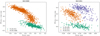 |
Fig. 1. Chromosome maps for NGC 2808 and NGC 1851. The identified populations of each cluster are labeled with different colors and symbols. For the type-II cluster NGC 1851, there is an additional population compared to NGC 2808. |
Type-II clusters contain stars that are enhanced in some particular heavy-elements, such as barium and lanthanum, possibly iron as well, compared to P1 and P2 stars (Marino et al. 2015). These metal-enhanced stars are found on the reddest part of the RGB in the color-magnitude diagram (see, e.g., Milone et al. 2017). For the Type-II clusters, we considered these stars as a third population (P3). The right panel in Fig. 1 shows our split into three populations for the type-II cluster NGC 1851. The position of P1 and P2 for NGC 1851 are similar to NGC 2808, but the third population has a distinct position on the upper-right region of the chromosome map.
We analyzed 25 globular clusters, six of which are considered type-II clusters. As briefly mentioned in Sect. 1, some type-II clusters might actually be the remnants of nuclear star clusters. However, Pfeffer et al. (2021) conclude that none of the type-II clusters in our sample are remnants of nuclear star clusters. Therefore, we treated them as globular clusters. A list of all clusters with the number of stars used in the analysis of the global kinematics, and the number of stars per population, are shown in Table 1. For NGC 1904, NGC 6266, NGC 6293, and NGC 6522 the necessary HUGS photometric data to separate their RGB stars into populations are not available. In these cases, we only derived the global kinematic properties.
Number of stars per cluster and population.
3.2. Kinematics
To study the kinematic differences between populations, we first used the radial velocities of all stars in the cluster to derive its global kinematics. Then we repeated the same procedure, including only the RGB stars assigned to specific populations. From the radial velocity data we created kinematic profiles and finally derived the ratio of ordered-over-random motion (v/σ)HL and a proxy for the spin parameter λR, HL. Both were evaluated at the half-light radius to characterize the strength of rotation for all clusters and each of their populations. We used a very similar approach to that described in Kamann et al. (2020), but we repeat the important assumptions and formulas below.
To create kinematic profiles, we needed to derive the rotational velocity, vrot, and the line-of-sight velocity dispersion, σlos, of each cluster as a function of radius. To derive these parameters, we employed the maximum-likelihood approach described in Kamann et al. (2018). We assumed that the line-of-sight stellar velocities at any position (x, y) can be approximated by a Gaussian with mean vlos and standard deviation σlos. To account for the position of each star within the cluster with respect to the rotation axis of that cluster, we parameterized the line-of-sight velocities according to vlos(r, θ) = vrot(r)sin(θ − θ0), where  is the distance from the cluster center, θ0 is the angle of the cluster rotation axis, and θ = atan2(y, x) is the position angle measured counterclockwise from north to east.
As described in Kamann et al. (2020), we used parametric and nonparametric models to analyze the stellar rotation velocities. For the nonparametric approach, we simply binned velocities radially and derived the rotation velocity and velocity dispersion for each bin. The parametric rotation profile, vrot, we employed is characteristic for systems that have undergone violent relaxation (Lynden-Bell 1967; Gott 1973):
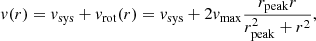
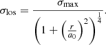
where vsys is the systematic velocity, vmax is the maximum rotation velocity reached at radial distance rpeak. The parametric dispersion profile we used is a Plummer (1911) profile,
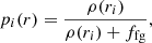
We differ in our approach to handling nonmember stars compared to Kamann et al. (2020). They used cluster membership probabilities that were derived from stellar metallicities and line-of-sight velocities, as described by Kamann et al. (2016). We cannot take the same approach, because we do not have metallicities for the additional Baumgardt & Hilker stars. We modified the method of membership determination in order to have consistent membership probabilities for stars from both data sets. In particular, we introduced a prior on the membership probability for each star pi that is related to the stellar surface density of the cluster ρ(ri) at the radial distance ri of that star from the cluster center according to
where ffg measures the fractional contribution of foreground sources to the observed source density. To describe the stellar surface density of each cluster, we used the LIMEPY models described in Gieles & Zocchi (2015), with parameters for each cluster as determined by de Boer et al. (2019). For NGC 6441 and NGC 6522 de Boer et al. (2019) do not provide any parameters for these models, so we chose to use King models (King 1966) with the necessary parameters of central concentration and core radius taken from Harris (1996, 2010 edition). We modified the likelihood function ℒi of each star i to not solely be based on the likelihood of the rotation and dispersion model ℒcl, i, but to include the membership probability pi as follows:

where ℒfg, i is the likelihood that star i is part of a foreground population. This foreground population was built from single stars included in a Besançon model (Robin et al. 2003) at the position of each cluster. The foreground likelihood for each star, ℒfg, i, is then defined as the superposition of Gaussian kernels for M simulated stars with line-of-sight velocities vfg, j:
where verr, i is the uncertainty of the measured line-of-sight velocities, vlos, i.
To maximize the likelihood of our model given the data, we used the Python package emcee from Foreman-Mackey et al. (2013), which is an implementation of the invariant Markov chain Monte Carlo (MCMC) ensemble sampler by Goodman & Weare (2010). Thinning the samples of each parameter by 16 ensures that the final set of values for each parameter is again uncorrelated. We calculated the best fit parameters as the median of each distribution of thinned samples. In accordance with the standard deviation of a Gaussian, the lower and upper uncertainties of each fitted parameter were calculated using the 16th and 84th percentile of the corresponding distribution. However, in some cases, the distribution of the maximum rotation velocity vmax may have a peak at zero and drop toward zero for larger values of vmax. In those cases we calculated an upper limit on the rotation velocity that corresponds to the 95th percentile of the distribution and the rotation angle could not be calculated. The actual fitting procedure for each cluster is performed as follows: First, the parametric models were fitted simultaneously to the line-of-sight velocities for the overall cluster including the Baumgardt & Hilker data, with the systematic velocity (vsys), rotation amplitude (vmax), rotation angle (θ0), rpeak, σmax, a0, and ffg as free parameters. The corresponding priors for each parameter are presented in Table A.1 with the subscript “o”. The priors on rpeak and a0 were chosen to exclude unphysical solutions for either small or large values of these parameters.
Second, the parametric models were fitted independently for each population of that cluster with vsys, vmax, θ0, rpeak, σmax, a0 as free parameters. The fraction of foreground stars ffg from the parametric fit of the overall cluster was used to derive membership probabilities for each star that are kept fixed. The priors of all fitted parameters are listed in Table A.1 with the subscript “p”. The radial extent of the separation in multiple populations is limited by the availability of HUGS photometry from Piotto et al. (2015) and Nardiello et al. (2018a), which is why the radial coverage of the velocity and dispersion profiles for each population is limited compared to the overall cluster. Therefore, we chose to apply strict priors on rpeak and a0 based on the distributions of samples from the parametric fit of the overall cluster. We chose to take a similar approach on vsys, since the systematic velocity should not vary between populations. Furthermore, we applied a soft prior in vmax that is based on the distributions of samples from the parametric fit of the overall cluster for vmax and σmax, and the escape velocity vesc of that cluster, where we used values for the escape velocities from Baumgardt & Hilker (2018).
Finally, the nonparametric model was fitted to the overall cluster and each of its populations with vsys, vmax, θ0 and σlos as free parameters per radial bin. The priors for each parameter are listed in Table A.2. Again, we chose to limit the systematic velocity vsys based on the results from the corresponding parametric fit. Additionally, we applied a prior on θ0 based on the value of θ0 from the corresponding parametric fit to ensure that the nonparametric profiles are consistent with the parametric profiles. We note that this approach introduces bias against depicting changes in the rotation axis with radius.
As described above, we only used the additional radial velocities from Baumgardt & Hilker (2018) in the analysis of the overall cluster, not its populations, because we were unable to split those stars into populations. Nonetheless, the inclusion of these data is still important since the strict priors on rpeak and a0 for the population fit are solely based on the fit of the whole cluster. Without the addition of that data, we would not be able to reliably derive these parameters for most clusters, as a result of the smaller radial range.
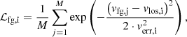
To quantify the effect of rotation, we calculated the ratio of ordered-over-random (v/σ)HL motion for each population in all clusters. Classically, this ratio is defined as the ratio between the maximum rotation velocity to the central velocity dispersion. However, because of the weaknesses of this approach mentioned by Binney (2005), we followed the definition of (v/σ)HL by Cappellari et al. (2007):
where rHL is the half-light radius of each cluster. Emsellem et al. (2007) highlight a potential shortcoming of using (v/σ)HL to characterize velocity fields, in that structurally different velocity fields can result in very similar values of (v/σ)HL. To address this issue, they introduce λR, HL as an alternative, which is a proxy for the spin parameter of the velocity field:
We calculated both parameters based on the rotation and dispersion profiles described in Eqs. (1) and (2) for each cluster and its populations to quantify kinematical differences between clusters and populations. For these calculations, we used the values of the half-light radius, rHL, from Harris (1996, 2010 edition). For each cluster and all of its populations, we used the global density profiles, ρ(r). For some clusters, the radial rotation profiles do not extend beyond the half-light radius. This could introduce some bias to the values of (v/σ)HL and λR, HL. However, as described earlier, we applied a strict prior on the radial scales of the rotation and dispersion profiles for each population based on the overall profile. Therefore, when we calculated (v/σ)HL and λR, HL based on the MCMC results of the radial rotation and dispersion profiles, we expect that any bias that may occur is correctly reflected in our uncertainties of these parameters. The kinematical model we employed to derive the rotation and dispersion profiles is not sensitive to structural differences between velocity fields of different clusters. Therefore, we expect that (v/σ)HL and λR, HL are qualitatively the same for each cluster with this model.
4. Results
4.1. Global kinematics
Figure 2 shows the radial rotation and dispersion profiles for NGC 2808. In the top panel of this figure, the global profiles for the cluster are presented, where the outermost radial velocity data points are from the stars in the Baumgardt & Hilker (2018) catalog. In the lower panels of this figure, the corresponding profiles are shown for each population. The continuous profiles and binned profiles shown here were each determined by fitting the respective model to line-of-sight velocities of single stars. The shaded area represents the 1σ uncertainty of each continuous profile and rotation angle. The dashed line indicates the value of the half-light radius of this cluster (Harris 1996, 2010 edition). The profiles for the other 24 globular clusters and their corresponding chromosome maps are displayed in Figs. A.1–A.24. The binned profiles highlight again that the radial extent of our data is limited to the center of each cluster. This could bias our ability to detect differences in kinematics between populations in the outer regions of the cluster. However, based on the work of Hénault-Brunet et al. (2015) we expect to find the largest differences between populations around the half-light radius of each cluster. Even closer to the center, differences should still be detectable. Nevertheless, the extension of our work to the outskirts of the clusters appears as a promising opportunity for future studies. Overall, the binned nonparametric profiles are in good agreement with the continuous parametric profiles. The largest discrepancies between these types of profiles are found close to the center, where the binned profiles indicate a rise in rotation velocity for some clusters (e.g., NGC 1904 and NGC 7089). Since the uncertainties of the binned rotation profiles are also the largest close to the center, it is uncertain whether this is a significant effect. We stress that the binned profiles are only used for visualization purposes and all following analyses were based on the parametric profiles. As mentioned in Sect. 3.2 the radial extent for the P1, P2 and P3 profiles is limited, which is revealed by the binned profiles. We used priors on the rpeak that are based on the parametric fit including all stars in the cluster. We used the parametric rotation and dispersion profiles to derive (v/σ)HL and λR, HL, according to Eqs. (6) and (7), for each cluster and its populations. Both of these values are integrals of these profiles up to the half-light radius of each cluster, which makes both parameters robust against changes in rpeak, as shown by Kamann et al. (2020). The fitted parameters and the values of (v/σ)HL and λR, HL for the populations of all clusters are listed in Table A.3. Since the value of vsys is close to zero for each cluster and its populations, it is not important for the subsequent analysis and is not discussed further.
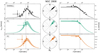 |
Fig. 2. Rotation and dispersion profiles for NGC 2808 and each of its populations. The rotation profiles for each population are shown on the left and the dispersion profiles on the right. The angle of rotation is shown in the center. The continuous profiles (solid lines) and binned profiles (symbols) shown here are each determined by fitting the respective model to line-of-sight velocities of single stars. The shaded area represents the 1σ uncertainty of each continuous profile and rotation angle. The dotted vertical line in each radial profile illustrates the half-light radius of NGC 2808. |
In Fig. 3 we show our values of (v/σ)HL as a function of the median relaxation time Trh of each cluster. The values for Trh are from Harris (1996, 2010 edition; see our Table A.3). For the global kinematics of the clusters, we find that there is a relationship between (v/σ)HL and the median relaxation time, in that for clusters with higher relaxation times we tend to get higher values in (v/σ)HL. In particular, for NGC 362, NGC 6397, NGC 6522 and NGC 6681 we do not find a significant sign of rotation and all of them have relaxation times of log10(Trh/yr) < 8.95. Similar relations between cluster rotation and relaxation time have been found by Kamann et al. (2018), Bianchini et al. (2018) and Sollima et al. (2019). This is to be expected if we assume that globular clusters are imprinted at birth with the angular momentum of their parent molecular clouds. Over time, this angular momentum is dissipated outward through two-body relaxation. In fact, numerical simulations show that star clusters can be rotating shortly after their birth (Mapelli 2017; Bekki 2019) and that the strength of rotation declines over time (Lahén et al. 2020). For several clusters in our sample, the relaxation times provided by Sollima & Baumgardt (2017) differ from those by Harris (1996, 2010 edition). Using the values provided by Sollima & Baumgardt (2017), we find a similar relation with our values of (v/σ)HL but the correlation is weaker.
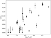 |
Fig. 3. Relation between rotation strength in (v/σ)HL and the median relaxation time, Trh, of each cluster taken from Harris (1996, 2010 edition) |
We find a linear relation between (v/σ)HL and λR, HL for all clusters and populations. This is shown in Fig. A.25. We find that the constant of proportionality is ≈0.8 for all cases. Since our kinematic model is not sensitive to structural differences in the velocity field of a cluster it is expected that (v/σ)HL and λR, HL are qualitatively the same. In the following, we only use (v/σ)HL to describe the kinematics of clusters and populations.
4.2. Differences between P1 and P2
To analyze P1 and P2 for differences in their kinematics, we compare the distributions of (v/σ)HL derived from the thinned MCMC samples for vmax, θ0, rpeak, σmax and a0 using Eqs. (1), (2) and (6). Figure 4 shows these distributions for all populations of each cluster. For NGC 1904, NGC 6266, NGC 6293, and NGC 6522, only the distribution for all stars is plotted because there is no separation into populations for these clusters.
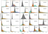 |
Fig. 4. Distributions of samples of (v/σ)HL, which describe the rotation strength for each cluster in this analysis. These distributions are shown for the overall cluster (gray) and each of its populations (P1:green, P2:orange, P3:violet). The 16th, 50th, and 84th percentile for each distribution are shown on top of the corresponding distribution. For distributions that peak at zero, only the 95th percentile is shown, to provide an upper limit on the rotation strength. |
For NGC 362, NGC 3201, NGC 6218, NGC 6254, NGC 6397, NGC 6624, NGC 6656, NGC 6681, NGC 6752, and NGC 7099 we find that the distributions of (v/σ)HL for P1 and P2 shown in Fig. 4 are consistent with zero. In these cases, we are unable to detect rotation for either population (see Table A.3 and the corresponding rotation profiles in the appendix). Based on our analysis, we find that our ability to detect rotation for any population depends mainly on two factors. First, the uncertainties of our analysis increase substantially for clusters with fewer than ∼200 stars per population (e.g., NGC 3201 and NGC 6218), resulting in a very broad distribution of (v/σ)HL. Second, if a cluster is slowly rotating ((v/σ)HL ≲ 0.05), it is challenging to constrain the rotation of its populations given our uncertainties. When both factors are present, as in the cases of NGC 6397 and NGC 6752, our analysis only provides broad upper limits on the rotation strength of each population.
For NGC 104, NGC 1851, NGC 2808, NGC 5286, NGC 5904, NGC 6093, NGC 6388, NGC 6541, NGC 7078, and NGC 7089 we are able to detect rotation for P1 or P2. All of these clusters fulfill the condition (v/σ)HL ≳ 0.05. NGC 6656 is the only other cluster in our sample that also fulfills this condition, but we are unable to detect rotation in P1 and P2 because its populations contain fewer than 200 stars. This shows that the global rotation of the cluster strongly affects the rotation of the individual populations, as expected. Based on the distributions of (v/σ)HL shown in Fig. 4, we find kinematic differences between P1 and P2 that are significant above a 1σ level for NGC 2808, NGC 6093, and NGC 7078. For NGC 6093 and NGC 7078 we find that P2 rotates faster than P1 at a confidence level of 1.5σ and 2.2σ, respectively, whereas P2 rotates more slowly than P1 in NGC 2808 at a confidence level of 1.8σ. For NGC 104, NGC 1851, NGC 5286, NGC 5904, NGC 6388, NGC 6541, and NGC 7089 the strength of rotation of P1 is consistent with that of P2.
Furthermore, we investigated whether the strength of rotation of P1 and P2 or their difference can be related to the relaxation time of the corresponding cluster. In the top and middle panel of Fig. 5 the values of (v/σ)HL are plotted against the relaxation time of the corresponding cluster for P1 and P2. For both P1 and P2, the strength of rotation only depends weakly on the relaxation time, if there is any correlation at all. Moreover, we do not see a correlation between the difference of rotation strength between P1 and P2 with relaxation time, which is illustrated in the bottom panel of Fig. 5. However, the significance of these results should be taken with a grain of salt, since we only find differences above the 1σ level for three clusters.
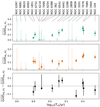 |
Fig. 5. Relation between rotation strength in (v/σ)HL of P1 and P2 and the median relaxation time, Trh, for each cluster taken from Harris (1996, 2010 edition), and the difference in rotation strength between P1 and P2 as a function of median relaxation time. |
In addition, we looked into possible connections between our kinematic differences and the radial concentration of P1 and P2. In fact, both NGC 6093 and NGC 7078 have been reported to contain a more centrally concentrated P1 compared to P2 according to Dalessandro et al. (2018) and Larsen et al. (2015), respectively. For both clusters, we find that P1 rotates more slowly than P2. However, Nardiello et al. (2018a) find no difference in concentration between P1 and P2 for NGC 7078. For NGC 104 (e.g., Milone et al. 2018a; Cordoni et al. 2020) and NGC 2808 (Dalessandro et al. 2019) P2 was found to be more centrally concentrated than P1. Whereas we do not find significant kinematic differences between P1 and P2 for NGC 104, we find that P1 rotates faster than P2 for NGC 2808. Overall, this could hint at a connection between kinematic differences and the radial concentration of multiple populations in globular clusters, that a population more centrally concentrated would rotate less. However, since we only find kinematic differences in three clusters and the information on the concentrations is only available for a small subset of our sample of clusters, additional data are needed to investigate this further. Furthermore, the observations of, for example, NGC 5272 (Lee & Sneden 2021), NGC 6205 (Johnson & Pilachowski 2012; Cordero et al. 2017), and NGC 6362 (Dalessandro et al. 2019, 2021) do not support this trend in our data, that more centrally concentrated populations rotate less.
4.3. Additional population in type-II clusters
The distributions of (v/σ)HL for type-II clusters are also shown in Fig. 4. For four of the six type-II clusters in our sample, we do not detect rotation in P3. For NGC 362, NGC 6656, and NGC 7089 this is most likely due to the low number of stars in P3 as discussed previously. For NGC 6388 P3 is populated well, but the global rotation of the cluster is very low. For NGC 1851 and NGC 5286 we detect rotation in P1, P2 and P3. For NGC 1851 we find that the distribution of (v/σ)HL for P3 is very similar to that of P1 and P2, whereas for NGC 5286, there might be a hint of P3 rotating faster than P1 and P2. However, the observed difference in (v/σ)HL is still within the 1σ uncertainty interval, so further data are needed to draw any solid conclusions. In particular, these results also do not give any clear hints on other formation scenarios for type-II clusters.
4.4. Notes on individual clusters
4.4.1. NGC 6093
For NGC 6093 we observe that rpeak varies between P1 and P2 (see Table A.3). While the values of rpeak for the whole cluster and P1 are consistent, the distribution of samples for rpeak of P2 peaks at a much smaller value, which is also apparent in the radial rotation profile in Fig. A.8. Furthermore, the distribution of rpeak for P2 is asymmetric and there is a strong anticorrelation between rpeak and vmax. This causes the asymmetry of (v/σ)HL in Fig. 4 for P2 of this cluster. As discussed in Sect. 4.1 the value of (v/σ)HL is generally robust to changes in rpeak. However, in this case the value of rpeak for P2 is very close to the center of that cluster, and it seems worthwhile to find out whether this has a significant effect on our results. If we apply a uniform prior on rpeak for P2, we find that the difference between P1 and P2 in (v/σ)HL is even larger and the asymmetry in the distribution of (v/σ)HL vanishes. If we fix the value of rpeak for P2 to that obtained for the whole cluster, the asymmetry also vanishes, but in this case (v/σ)HL is consistent with that value for P1. This cluster has already been analyzed for kinematic differences between populations based on MUSE data, with a very similar approach as the one presented here by Kamann et al. (2020). They do not find this peculiar behavior of P2 for that cluster, because they used a different population split than the one used here. Notably, they also used individual population density profiles when calculating (v/σ)HL for their populations and not the global density profile of that cluster. Kamann et al. (2020) split the cluster in three populations, where our P1 is consistent with their primordial population and our P2 includes their intermediate and extreme populations. If we average their values of (v/σ)HL for the intermediate and extreme population, the result is consistent with the value of (v/σ)HL they obtained for the primordial population. If we consider that Kamann et al. (2020) fixed the radial scale of each population, our results are consistent with theirs in that we do not find significant kinematic differences between P1 and P2 if the radial scale is fixed to that of the global profile. However, there is no physical reason for why the radial scale of P2 cannot be different from that of P1.
4.4.2. NGC 2808 and NGC 7078
For NGC 2808 and NGC 7078 we find differences above the 1σ level in (v/σ)HL and the rotation profiles of their populations, whereas the dispersion profiles do not differ significantly. For NGC 7078 we observe that P2 rotates faster than P1. Qualitatively, this behavior is similar to that of NGC 6093 and NGC 6205, where differences of this type between similar populations have also been reported by Kamann et al. (2020) and Cordero et al. (2017), respectively. For NGC 2808 we find the opposite in that P1 rotates faster than P2.
To further investigate the relationship between the populations in the chromosome maps and their kinematic differences for NGC 2808 and NGC 7078, we decided to reiterate the analysis with different population splits. Incidentally, the structure of the chromosome maps of these clusters allowed us to distinguish between four populations (P1, P2’, P3’, and P4’) for NGC 2808 (Milone et al. 2015; Latour et al. 2019) and three populations (P1, P2’, and P3’) for NGC 7078 (Nardiello et al. 2018b). Compared to Milone et al. (2015) our P2’, P3’, and P4’ in NGC 2808 are equivalent to their populations C, D, and E, while our P1’ is their populations A and B combined. For NGC 7078, our P2’ is equivalent to population B by Nardiello et al. (2018b), whereas our P1’ corresponds to their populations A and D and our population P3’ is equal to their populations C and E. We did not split P1’ for both clusters and P3’ for NGC 7078 any further to ensure that there are still enough stars per population to get meaningful results from our analysis. These populations according to our splitting are shown in the chromosome maps in the upper panels of Fig. 6, whereas the distributions of (v/σ)HL for these populations are depicted in the lower panels of that figure. For NGC 2808 we find that P2’, P3’ and P4’ do not differ in their rotation significantly, but the difference between these three populations and P1’ is larger than 1σ. For NGC 7078 the value of (v/σ)HL of P3’ stars is consistent with that of P1’ and P2’ stars, but the difference between P1’ stars and P2’ is larger than 1σ. Therefore, we do not find a general trend of (v/σ)HL along these populations.
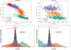 |
Fig. 6. Chromosome maps of NGC 2808 and NGC 7078, with additional population splits (top) and the corresponding distributions of samples of (v/σ)HL (bottom). For NGC 2808 the original P2 is split into three subpopulations (P2′, P3′, and P4′), whereas P2 of NGC 7078 is split into two subpopulations (P2′and P3′) according to the respective morphology of the chromosome maps. |
NGC 7078 has been analyzed for kinematic differences in populations by Szigeti et al. (2021). They used high precision radial velocity data from the SDSS-IV APOGEE-2 survey for 138 stars in NGC 7078 to measure its rotation amplitude as a function of position angle for the whole cluster and two populations that were identified based on single element abundance changes. They derived the angular rotation profile of NGC 7078 by splitting the cluster into two halves through the cluster center. This line of separation is rotated in small angular increments, and the difference in mean radial velocity, ΔV, between both halves is calculated at each step. If the cluster is rotating, the relation between velocity difference, ΔV, and position angle relative to the rotation axis, α, is ΔV = 2vrot ⋅ sin(α). The global rotation amplitude and rotation angle that they find agree with our values for vmax and θ0 for the whole cluster. Furthermore, they find no kinematic difference between their two populations, which is in contrast to our results. To investigate this further, we decided to apply their method to our data. Their method may only be applied to a fully sampled area that is symmetric with respect to the position angle. To ensure that our data complied with those restrictions, we filtered our stars to make the covered area of the cluster circular. When we apply their method to our filtered data for P1 and P2, we find rotation amplitudes and rotation angles that are consistent with our radial rotation curves for P1 and P2. The corresponding angular rotation profiles and the spatial coverage of the cluster are shown in Fig. A.26. In particular, we still find kinematic differences between P1 and P2. One striking difference between their data and ours is that we have 390 and 697 stars in P1 and P2, compared to their 33 and 49 stars in those populations. To investigate this further, we decreased the number of stars by randomly sampling from P1 and P2 and then applied their method again. Figure A.27 shows three of these angular rotation profiles and the spatial coverage of the cluster. We find that with so few stars, this method results in a wide range of fundamentally different profiles, presumably because the method is very sensitive to single stars. Probably the uncertainties of the differential rotation profiles are underestimated because the strong correlations between different values in those profiles are generally not taken into account. Together with our much larger sample of analyzed stars, this could be the cause for the discrepancies between our results and those from Szigeti et al. (2021).
NGC 2808 has not been analyzed for differences in its radial rotation and dispersion profiles yet, but Bellini et al. (2015) found differences in the radial anisotropy profiles for this cluster, by using proper motion data. Given that this cluster shows kinematic differences using both radial velocities and proper motion data, it would be very interesting to combine both data sets and analyze the 3D stellar velocities of this cluster for differences between multiple populations.
4.4.3. NGC 104 and NGC 5904
Neither Milone et al. (2018b) nor Cordoni et al. (2020) find differences in the rotation amplitude between the populations of NGC 104, which agrees with our results. For NGC 5904 Cordoni et al. (2020) do not observe any differences in rotation amplitude, but they do find differences in the phase of their rotation curves. These phase differences translate to a differing angle of rotation. We do not find any significant differences in rotation amplitudes for NGC 5904 either, but we also do not find a significant difference in the angle of rotation between P1 and P2.
4.5. Random sampling of the chromosome map
To further analyze the solidity of our results for NGC 2808, NGC 6093, and NGC 7078 and to evaluate our uncertainty estimations, we randomly sampled the chromosome maps of these clusters to create random populations P1 and P2. To ensure comparability to the original population split, we used the same number of stars per population as in the original separations (see Table 1). To achieve statistically relevant results, we created 100 random population pairs for each cluster. We calculated the rotation and dispersion profiles and derived (v/σ)HL for each of these random populations, as described in Sect. 3.2. As a result, we calculated 100 values of (v/σ)HL for each population of each cluster, which are shown in the upper panels of Fig. 7. It is apparent that the distributions for P1 and P2 for each cluster have the same median value. This shows that, on average, we do not find kinematic differences when randomly sampling the chromosome map. We also find that the distributions of  obtained with the random sampling are broader for smaller numbers of stars per population, as expected. In the lower panels of Fig. 7 we show the differences of
  between P1 and P2 obtained from the random sampling. As expected, these distributions are centered around zero. We also indicated the observed differences for NGC 2808, NGC 6093 and NGC 7078. The observed differences lie outside the 1σ regions of the distributions, which supports the solidity of our uncertainty estimations and indicates that the kinematic differences that we find for NGC 2808, NGC 6093, and NGC 7078 are truly connected to the populations defined in the chromosome maps.
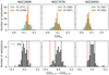 |
Fig. 7. Values of |

5. Conclusion and outlook
We created and analyzed the rotation and dispersion profiles of 25 Galactic globular clusters in a search for kinematic differences between different populations within each cluster. Based on these kinematic profiles, we derived the rotation strength in terms of the ratio of ordered-over-random motion, (v/σ)HL, evaluated at the half-light radius, for each cluster and its populations to quantify kinematic differences. For NGC 362, NGC 6397, NGC 6522, and NGC 6681, we find no significant global rotation when using all stars in these clusters. For NGC 104, NGC 1851, NGC 2808, NGC 5286, NGC5904, NGC 6093, NGC 6388, NGC 6541, NGC 7078, and NGC 7089, we are able to detect rotation in at least one of their populations. For three clusters we find differences above the 1σ level: for NGC 6093 and NGC 7078 we find that P2 stars rotate faster than P1 stars, whereas we find the opposite for NGC 2808.
Our results do not give a clear hint as to the formation scenario of multiple populations in globular clusters. We find support for both multi-epoch and single-epoch formation scenarios in our data. For multi-epoch formation scenarios, we expect to find that P2 rotates faster than P1, which matches our results for NGC 6093 and NGC 7078. Assuming a single-epoch formation scenario, it follows that P1 rotates faster than P2, which is what we find for NGC 2808. However, the kinematic differences that we find are still relatively uncertain at confidence levels of ≲2σ, so further data are needed for a definitive answer. We find further support for both scenarios if we consider clusters with kinematical variations between P1 and P2 below the 1σ level. While we find that the rotation strength of each cluster is positively correlated with the median relaxation time, the correlation between relaxation time and the rotation strength of P1 or P2 is weak at best, and we do not see a correlation of the kinematical difference between P1 and P2 with relaxation time. Based on our analysis, neither of the two types of formation scenarios for multiple populations in globular clusters is favored. As discussed in Bastian & Lardo (2018), none of the formation scenarios put forward to date is able to explain all the observations. It is also possible that the formation of multiple populations does not affect the rotation of either population in a way that we are able to observe. However, it would be very interesting to see what primordial differences between P1 and P2 are consistent with the differences between the populations that we find.
To get a better understanding of the formation scenarios of multiple populations and their kinematics in general, there are several problems worth addressing. For many clusters in our sample, we were unable to detect rotation for P1 or P2. However, since most clusters are rotating overall, we suspect that at least one population should also be rotating for most clusters. As mentioned in Sect. 4.1, we are generally unable to detect rotation in P1 or P2 if the overall cluster is already rotating slowly with (v/σ)HL ≲ 0.05 or when the number of stars per population is on the order of 200 stars or fewer. The results for NGC 6656 and NGC 3201 in particular could be significantly improved by increasing the number of stars per population, since these clusters are rotating fast enough to overcome that limitation. One way to tackle this issue is to determine the population tags directly from the spectra. An alternative would be to add additional photometric data and thus be able to assign more stars to their respective population. This would be especially useful outside the core of each cluster, where radial velocity measurements of stars are available (e.g., Baumgardt & Hilker 2018), but these stars have not been separated into populations yet. Leitinger et al. (2023) are currently working on using ground-based photometry to split the populations and derive density profiles for each population in globular clusters. When we included their additional population tags for NGC 7078, we observed small changes in the distribution of (v/σ)HL, but nothing significant since the number of stars per population is already comparatively large for that cluster. Nonetheless, it seems worthwhile to pursue that approach, since it also increases the radial range of the population data. It is possible that this could increase the accuracy of measurements of the rotation in P1 and P2 substantially. Another possibility for a future work would be to use density profiles per population to derive the rotation strength. Using data from Leitinger et al. (2023), we checked whether our results for NGC 7078 change if we use their density profiles for P1 and P2, but we still find that P2 rotates faster than P1 with a difference larger than 1σ. However, if the populations have the same rotation and dispersion curves but different concentrations, then we would expect to find kinematic differences between them. This is because the observed kinematics at a given projected radius correspond to a different intrinsic radius relative to the cluster center. Ultimately, one needs more sophisticated models to understand all the details.
Acknowledgments
SM, FG, ML, PMW and SD acknowledge funding from the Deutsche Forschungsgemeinschaft (grant LA 4383/4-1, DR 281/35-1 and KA 4537/2-1) and by the BMBF from the ErUM program through grants 05A14MGA, 05A17MGA, 05A20MGA and 05A20BAB. SK and RP gratefully acknowledge funding from UKRI in the form of a Future Leaders Fellowship (grant no. MR/T022868/1).
References
- Anderson, J., Sarajedini, A., Bedin, L. R., et al. 2008, AJ, 135, 2055 [Google Scholar]
- Bacon, R., Accardo, M., Adjali, L., et al. 2010, SPIE Conf. Ser., 7735, 773508 [Google Scholar]
- Bastian, N., & Lardo, C. 2018, ARA&A, 56, 83 [Google Scholar]
- Bastian, N., Lamers, H. J. G. L. M., de Mink, S. E., et al. 2013, MNRAS, 436, 2398 [CrossRef] [Google Scholar]
- Baumgardt, H., & Hilker, M. 2018, MNRAS, 478, 1520 [Google Scholar]
- Bekki, K. 2019, A&A, 622, A53 [NASA ADS] [CrossRef] [EDP Sciences] [Google Scholar]
- Bellini, A., Vesperini, E., Piotto, G., et al. 2015, ApJ, 810, L13 [NASA ADS] [CrossRef] [Google Scholar]
- Bianchini, P., van de Ven, G., Norris, M. A., Schinnerer, E., & Varri, A. L. 2016, MNRAS, 458, 3644 [NASA ADS] [CrossRef] [Google Scholar]
- Bianchini, P., van der Marel, R. P., del Pino, A., et al. 2018, MNRAS, 481, 2125 [Google Scholar]
- Binney, J. 2005, MNRAS, 363, 937 [Google Scholar]
- Cadelano, M., Dalessandro, E., Salaris, M., et al. 2022, ApJ, 924, L2 [NASA ADS] [CrossRef] [Google Scholar]
- Cappellari, M., Emsellem, E., Bacon, R., et al. 2007, MNRAS, 379, 418 [Google Scholar]
- Carretta, E., Bragaglia, A., Gratton, R. G., et al. 2009, A&A, 505, 117 [NASA ADS] [CrossRef] [EDP Sciences] [Google Scholar]
- Carretta, E., Bragaglia, A., Gratton, R. G., et al. 2010a, A&A, 516, A55 [NASA ADS] [CrossRef] [EDP Sciences] [Google Scholar]
- Carretta, E., Gratton, R. G., Lucatello, S., et al. 2010b, ApJ, 722, L1 [NASA ADS] [CrossRef] [Google Scholar]
- Cordero, M. J., Hénault-Brunet, V., Pilachowski, C. A., et al. 2017, MNRAS, 465, 3515 [NASA ADS] [CrossRef] [Google Scholar]
- Cordoni, G., Milone, A. P., Mastrobuono-Battisti, A., et al. 2020, ApJ, 889, 18 [Google Scholar]
- Cottrell, P. L., & Da Costa, G. S. 1981, ApJ, 245, L79 [NASA ADS] [CrossRef] [Google Scholar]
- Dalessandro, E., Lapenna, E., Mucciarelli, A., et al. 2016, ApJ, 829, 77 [NASA ADS] [CrossRef] [Google Scholar]
- Dalessandro, E., Cadelano, M., Vesperini, E., et al. 2018, ApJ, 859, 15 [NASA ADS] [CrossRef] [Google Scholar]
- Dalessandro, E., Cadelano, M., Vesperini, E., et al. 2019, ApJ, 884, L24 [Google Scholar]
- Dalessandro, E., Raso, S., Kamann, S., et al. 2021, MNRAS, 506, 813 [CrossRef] [Google Scholar]
- de Boer, T. J. L., Gieles, M., Balbinot, E., et al. 2019, MNRAS, 485, 4906 [Google Scholar]
- Decressin, T., Charbonnel, C., & Meynet, G. 2007a, A&A, 475, 859 [CrossRef] [EDP Sciences] [Google Scholar]
- Decressin, T., Meynet, G., Charbonnel, C., Prantzos, N., & Eksträm, S. 2007b, A&A, 464, 1029 [NASA ADS] [CrossRef] [EDP Sciences] [Google Scholar]
- Emsellem, E., Cappellari, M., Krajnović, D., et al. 2007, MNRAS, 379, 401 [Google Scholar]
- Foreman-Mackey, D., Hogg, D. W., Lang, D., & Goodman, J. 2013, PASP, 125, 306 [Google Scholar]
- Gieles, M., & Zocchi, A. 2015, MNRAS, 454, 576 [NASA ADS] [CrossRef] [Google Scholar]
- Gieles, M., Charbonnel, C., Krause, M. G. H., et al. 2018, MNRAS, 478, 2461 [Google Scholar]
- Giesers, B., Kamann, S., Dreizler, S., et al. 2019, A&A, 632, A3 [NASA ADS] [CrossRef] [EDP Sciences] [Google Scholar]
- Goodman, J., & Weare, J. 2010, Commun. Appl. Math. Comput. Sci., 5, 65 [Google Scholar]
- Gott, R. J., III 1973, ApJ, 186, 481 [NASA ADS] [CrossRef] [Google Scholar]
- Harris, W. E. 1996, AJ, 112, 1487 [Google Scholar]
- Hénault-Brunet, V., Gieles, M., Agertz, O., & Read, J. I. 2015, MNRAS, 450, 1164 [CrossRef] [Google Scholar]
- Husser, T.-O., Wende-von Berg, S., Dreizler, S., et al. 2013, A&A, 553, A6 [NASA ADS] [CrossRef] [EDP Sciences] [Google Scholar]
- Husser, T.-O., Kamann, S., Dreizler, S., et al. 2016, A&A, 588, A148 [NASA ADS] [CrossRef] [EDP Sciences] [Google Scholar]
- Johnson, C. I., & Pilachowski, C. A. 2012, ApJ, 754, L38 [NASA ADS] [CrossRef] [Google Scholar]
- Kamann, S., Wisotzki, L., & Roth, M. M. 2013, A&A, 549, A71 [NASA ADS] [CrossRef] [EDP Sciences] [Google Scholar]
- Kamann, S., Husser, T.-O., Brinchmann, J., et al. 2016, A&A, 588, A149 [NASA ADS] [CrossRef] [EDP Sciences] [Google Scholar]
- Kamann, S., Husser, T.-O., Dreizler, S., et al. 2018, MNRAS, 473, 5591 [NASA ADS] [CrossRef] [Google Scholar]
- Kamann, S., Dalessandro, E., Bastian, N., et al. 2020, MNRAS, 492, 966 [NASA ADS] [CrossRef] [Google Scholar]
- King, I. R. 1966, AJ, 71, 64 [Google Scholar]
- Lahén, N., Naab, T., Johansson, P. H., et al. 2020, ApJ, 904, 71 [CrossRef] [Google Scholar]
- Larsen, S. S., Baumgardt, H., Bastian, N., et al. 2015, ApJ, 804, 71 [NASA ADS] [CrossRef] [Google Scholar]
- Latour, M., Husser, T.-O., Giesers, B., et al. 2019, A&A, 631, A14 [NASA ADS] [CrossRef] [EDP Sciences] [Google Scholar]
- Lee, J.-W., & Sneden, C. 2021, ApJ, 909, 167 [NASA ADS] [CrossRef] [Google Scholar]
- Leitinger, E., Baumgardt, H., Cabrera-Ziri, I., Hilker, M., & Pancino, E. 2023, MNRAS, 520, 1456 [NASA ADS] [CrossRef] [Google Scholar]
- Libralato, M., Bellini, A., Piotto, G., et al. 2019, ApJ, 873, 109 [NASA ADS] [CrossRef] [Google Scholar]
- Lynden-Bell, D. 1967, MNRAS, 136, 101 [Google Scholar]
- Mapelli, M. 2017, MNRAS, 467, 3255 [NASA ADS] [CrossRef] [Google Scholar]
- Marino, A. F., Milone, A. P., Karakas, A. I., et al. 2015, MNRAS, 450, 815 [NASA ADS] [CrossRef] [Google Scholar]
- Martocchia, S., Niederhofer, F., Dalessandro, E., et al. 2018a, MNRAS, 477, 4696 [NASA ADS] [CrossRef] [Google Scholar]
- Martocchia, S., Cabrera-Ziri, I., Lardo, C., et al. 2018b, MNRAS, 473, 2688 [NASA ADS] [CrossRef] [Google Scholar]
- Milone, A. P., Bedin, L. R., Piotto, G., & Anderson, J. 2009, A&A, 497, 755 [NASA ADS] [CrossRef] [EDP Sciences] [Google Scholar]
- Milone, A. P., Marino, A. F., Piotto, G., et al. 2015, ApJ, 808, 51 [NASA ADS] [CrossRef] [Google Scholar]
- Milone, A. P., Piotto, G., Renzini, A., et al. 2017, MNRAS, 464, 3636 [Google Scholar]
- Milone, A. P., Marino, A. F., Di Criscienzo, M., et al. 2018a, MNRAS, 477, 2640 [Google Scholar]
- Milone, A. P., Marino, A. F., Mastrobuono-Battisti, A., & Lagioia, E. P. 2018b, MNRAS, 479, 5005 [NASA ADS] [CrossRef] [Google Scholar]
- Mucciarelli, A., Origlia, L., Ferraro, F. R., & Pancino, E. 2009, ApJ, 695, L134 [NASA ADS] [CrossRef] [Google Scholar]
- Nardiello, D., Libralato, M., Piotto, G., et al. 2018a, MNRAS, 481, 3382 [NASA ADS] [CrossRef] [Google Scholar]
- Nardiello, D., Milone, A. P., Piotto, G., et al. 2018b, MNRAS, 477, 2004 [NASA ADS] [CrossRef] [Google Scholar]
- Pfeffer, J., Lardo, C., Bastian, N., Saracino, S., & Kamann, S. 2021, MNRAS, 500, 2514 [Google Scholar]
- Piotto, G., Milone, A. P., Bedin, L. R., et al. 2015, AJ, 149, 91 [Google Scholar]
- Plummer, H. C. 1911, MNRAS, 71, 460 [Google Scholar]
- Renzini, A. 2013, Mem. Soc. Astron. It., 84, 162 [NASA ADS] [Google Scholar]
- Richer, H. B., Heyl, J., Anderson, J., et al. 2013, ApJ, 771, L15 [NASA ADS] [CrossRef] [Google Scholar]
- Robin, A. C., Reylé, C., Derrière, S., & Picaud, S. 2003, A&A, 409, 523 [NASA ADS] [CrossRef] [EDP Sciences] [Google Scholar]
- Sarajedini, A., Bedin, L. R., Chaboyer, B., et al. 2007, AJ, 133, 1658 [Google Scholar]
- Sollima, A., & Baumgardt, H. 2017, MNRAS, 471, 3668 [NASA ADS] [CrossRef] [Google Scholar]
- Sollima, A., Baumgardt, H., & Hilker, M. 2019, MNRAS, 485, 1460 [Google Scholar]
- Szigeti, L., Mészáros, S., Szabó, G. M., et al. 2021, MNRAS, 504, 1144 [NASA ADS] [CrossRef] [Google Scholar]
- Tiongco, M. A., Vesperini, E., & Varri, A. L. 2019, MNRAS, 487, 5535 [NASA ADS] [CrossRef] [Google Scholar]
- Vesperini, E., McMillan, S. L. W., D’Antona, F., & D’Ercole, A. 2013, MNRAS, 429, 1913 [Google Scholar]
- Weilbacher, P. M., Palsa, R., Streicher, O., et al. 2020, A&A, 641, A28 [NASA ADS] [CrossRef] [EDP Sciences] [Google Scholar]
Appendix A: Additional tables and figures
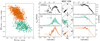 |
Fig. A.1. Chromosome maps and rotation and dispersion profiles for NGC 104 and each of its populations. The rotation profiles for each population are shown on the left and the dispersion profiles on the right. The angle of rotation is shown in the center. |
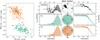 |
Fig. A.10. Continuation of Fig. A.1 for NGC 6254. |
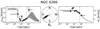 |
Fig. A.11. Continuation of Fig. A.1 for NGC 6266. |
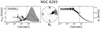 |
Fig. A.12. Continuation of Fig. A.1 for NGC 6293. |
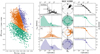 |
Fig. A.13. Continuation of Fig. A.1 for NGC 6388. |
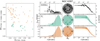 |
Fig. A.14. Continuation of Fig. A.1 for NGC 6397. |
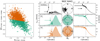 |
Fig. A.15. Continuation of Fig. A.1 for NGC 6441. |
 |
Fig. A.16. Continuation of Fig. A.1 for NGC 6522. |
 |
Fig. A.17. Continuation of Fig. A.1 for NGC 6541. |
 |
Fig. A.18. Continuation of Fig. A.1 for NGC 6624. |
 |
Fig. A.19. Continuation of Fig. A.1 for NGC 6656. |
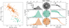 |
Fig. A.20. Continuation of Fig. A.1 for NGC 6681. |
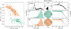 |
Fig. A.21. Continuation of Fig. A.1 for NGC 6752. |
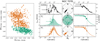 |
Fig. A.22. Continuation of Fig. A.1 for NGC 7078. |
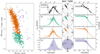 |
Fig. A.23. Continuation of Fig. A.1 for NGC 7089. |
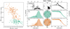 |
Fig. A.24. Continuation of Fig. A.1 for NGC 7099. |
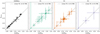 |
Fig. A.25. Derived values of λR, HL plotted against (v/σ)HL for the overall cluster and each population with a linear fit. |
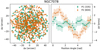 |
Fig. A.26. Differential rotation profile for P1 and P2 of NGC 7078. The difference in mean radial velocity between the two subsets of stars is plotted against the position angle of their line of separation. |
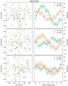 |
Fig. A.27. Differential rotation profile for randomly sampled stars of P1 and P2 for NGC 7078. The difference in mean radial velocity between the two subsets of stars is plotted against the position angle of their line of separation. |
Priors of the parametric fit described in Sect. 3.2.
Priors of the nonparametric fit described in Sect. 3.2.
Median and upper limits of the parameter distributions for the parametric model of each cluster.
All Tables
Median and upper limits of the parameter distributions for the parametric model of each cluster.
All Figures
|
Fig. 1. Chromosome maps for NGC 2808 and NGC 1851. The identified populations of each cluster are labeled with different colors and symbols. For the type-II cluster NGC 1851, there is an additional population compared to NGC 2808. |
| In the text | |
|
Fig. 2. Rotation and dispersion profiles for NGC 2808 and each of its populations. The rotation profiles for each population are shown on the left and the dispersion profiles on the right. The angle of rotation is shown in the center. The continuous profiles (solid lines) and binned profiles (symbols) shown here are each determined by fitting the respective model to line-of-sight velocities of single stars. The shaded area represents the 1σ uncertainty of each continuous profile and rotation angle. The dotted vertical line in each radial profile illustrates the half-light radius of NGC 2808. |
| In the text | |
|
Fig. 3. Relation between rotation strength in (v/σ)HL and the median relaxation time, Trh, of each cluster taken from Harris (1996, 2010 edition) |
| In the text | |
|
Fig. 4. Distributions of samples of (v/σ)HL, which describe the rotation strength for each cluster in this analysis. These distributions are shown for the overall cluster (gray) and each of its populations (P1:green, P2:orange, P3:violet). The 16th, 50th, and 84th percentile for each distribution are shown on top of the corresponding distribution. For distributions that peak at zero, only the 95th percentile is shown, to provide an upper limit on the rotation strength. |
| In the text | |
|
Fig. 5. Relation between rotation strength in (v/σ)HL of P1 and P2 and the median relaxation time, Trh, for each cluster taken from Harris (1996, 2010 edition), and the difference in rotation strength between P1 and P2 as a function of median relaxation time. |
| In the text | |
|
Fig. 6. Chromosome maps of NGC 2808 and NGC 7078, with additional population splits (top) and the corresponding distributions of samples of (v/σ)HL (bottom). For NGC 2808 the original P2 is split into three subpopulations (P2′, P3′, and P4′), whereas P2 of NGC 7078 is split into two subpopulations (P2′and P3′) according to the respective morphology of the chromosome maps. |
| In the text | |
|
Fig. 7. Values of |
| In the text | |
|
Fig. A.1. Chromosome maps and rotation and dispersion profiles for NGC 104 and each of its populations. The rotation profiles for each population are shown on the left and the dispersion profiles on the right. The angle of rotation is shown in the center. |
| In the text | |
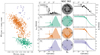 |
Fig. A.2. Continuation of Fig. A.1 for NGC 362. |
| In the text | |
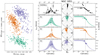 |
Fig. A.3. Continuation of Fig. A.1 for NGC 1851. |
| In the text | |
 |
Fig. A.4. Continuation of Fig. A.1 for NGC 1904. |
| In the text | |
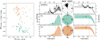 |
Fig. A.5. Continuation of Fig. A.1 for NGC 3201. |
| In the text | |
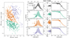 |
Fig. A.6. Continuation of Fig. A.1 for NGC 5286. |
| In the text | |
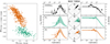 |
Fig. A.7. Continuation of Fig. A.1 for NGC 5904. |
| In the text | |
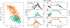 |
Fig. A.8. Continuation of Fig. A.1 for NGC 6093. |
| In the text | |
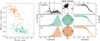 |
Fig. A.9. Continuation of Fig. A.1 for NGC 6218. |
| In the text | |
|
Fig. A.10. Continuation of Fig. A.1 for NGC 6254. |
| In the text | |
|
Fig. A.11. Continuation of Fig. A.1 for NGC 6266. |
| In the text | |
|
Fig. A.12. Continuation of Fig. A.1 for NGC 6293. |
| In the text | |
|
Fig. A.13. Continuation of Fig. A.1 for NGC 6388. |
| In the text | |
|
Fig. A.14. Continuation of Fig. A.1 for NGC 6397. |
| In the text | |
|
Fig. A.15. Continuation of Fig. A.1 for NGC 6441. |
| In the text | |
|
Fig. A.16. Continuation of Fig. A.1 for NGC 6522. |
| In the text | |
|
Fig. A.17. Continuation of Fig. A.1 for NGC 6541. |
| In the text | |
|
Fig. A.18. Continuation of Fig. A.1 for NGC 6624. |
| In the text | |
|
Fig. A.19. Continuation of Fig. A.1 for NGC 6656. |
| In the text | |
|
Fig. A.20. Continuation of Fig. A.1 for NGC 6681. |
| In the text | |
|
Fig. A.21. Continuation of Fig. A.1 for NGC 6752. |
| In the text | |
|
Fig. A.22. Continuation of Fig. A.1 for NGC 7078. |
| In the text | |
|
Fig. A.23. Continuation of Fig. A.1 for NGC 7089. |
| In the text | |
|
Fig. A.24. Continuation of Fig. A.1 for NGC 7099. |
| In the text | |
|
Fig. A.25. Derived values of λR, HL plotted against (v/σ)HL for the overall cluster and each population with a linear fit. |
| In the text | |
|
Fig. A.26. Differential rotation profile for P1 and P2 of NGC 7078. The difference in mean radial velocity between the two subsets of stars is plotted against the position angle of their line of separation. |
| In the text | |
|
Fig. A.27. Differential rotation profile for randomly sampled stars of P1 and P2 for NGC 7078. The difference in mean radial velocity between the two subsets of stars is plotted against the position angle of their line of separation. |
| In the text | |
Current usage metrics show cumulative count of Article Views (full-text article views including HTML views, PDF and ePub downloads, according to the available data) and Abstracts Views on Vision4Press platform.
Data correspond to usage on the plateform after 2015. The current usage metrics is available 48-96 hours after online publication and is updated daily on week days.
Initial download of the metrics may take a while.