| Issue |
A&A
Volume 671, March 2023
|
|
|---|---|---|
| Article Number | A16 | |
| Number of page(s) | 20 | |
| Section | Celestial mechanics and astrometry | |
| DOI | https://doi.org/10.1051/0004-6361/202142929 | |
| Published online | 28 February 2023 | |
Carte du Ciel and Gaia
I. Astrometry★
1
Finnish Geospatial Research Institute,
Geodeetinrinne 2,
02430
Masala,
Finland
e-mail: This email address is being protected from spambots. You need JavaScript enabled to view it.
2
European Space Research and Technology Centre (ESA/ESTEC),
Keplerlaan 1,
2201
AZ Noordwijk,
The Netherlands
3
European Space Astronomy Centre (ESA/ESAC), Camino bajo del Castillo s/n, Urbanizacion Villafranca del Castillo,
Villanueva de la Canada,
28692
Madrid,
Spain
4
European Southern Observatory (ESO),
Karl-Schwarzschild-Strasse 2,
85748
Garching bei München,
Germany
5
Department of Physics,
Gustaf Hällstömin katu 2A,
00014
University of Helsinki, Helsinki,
Finland
6
Department of Astrophysical Sciences, Princeton University,
Princeton, NJ
08544,
USA
Received:
16
December
2021
Accepted:
20
October
2022
Abstract
Context. The Carte du Ciel archive at the University of Helsinki enables us to see the sky as it was about 120 yr ago. The archive consists of single-exposure and triple-exposure plates between epochs 1896.8–1925.8.
Aims. Our main aim is to find binary and multiple stars by combining Carte du Ciel and Gaia data.
Methods. The plates were digitised with a commercial digital camera. We used Gaia data to calculate predicted coordinates of stars at the epoch of each plate. These stars were used as reference stars to fit astrometry for each plate, giving fitted coordinates for stars on the Carte du Ciel plates. If the predicted and fitted coordinates differed at a significant level, we classified the star as a non-single star, for which the proper motion values given in the Gaia catalogue can be unreliable.
Results. We find that several astrometric quality indicators of Gaia indicate that the uncertainties of Gaia’s single-star model fit are, in general, larger for our non-single-star candidates. The percentage of our non-single-star candidates, which are in the catalogues of known binary stars, is relatively low, ~10% at maximum.
Conclusions. The combination of the Carte du Ciel and Gaia data can be used to identify candidates of non-single stars. We propose that the sources with a significant difference between the predicted and fitted coordinates are long-period binaries, although astrophysical and/or instrumental effects as origin for the coordinate difference cannot be excluded for individual cases.
Key words: astrometry / proper motions / binaries: general / surveys / catalogs / techniques: image processing
Tables 2 to 13 are only available at the CDS via anonymous ftp to cdsarc.cds.unistra.fr (130.79.128.5) or via https://cdsarc.cds.unistra.fr/viz-bin/cat/J/A+A/671/A16
© The Authors 2023
 Open Access article, published by EDP Sciences, under the terms of the Creative Commons Attribution License (https://creativecommons.org/licenses/by/4.0), which permits unrestricted use, distribution, and reproduction in any medium, provided the original work is properly cited.
This article is published in open access under the Subscribe to Open model. This email address is being protected from spambots. You need JavaScript enabled to view it. to support open access publication.
1 Introduction
In the year 1887, in a meeting in Paris, more than 50 astronomers agreed on a project to map the sky on photographic plates. In the first step, the aim was to produce the Astrographic Catalogue down to magnitude limit 11. This part of the project was completed in the early twentieth century. The second part of the project, known as the Carte du Ciel (hereafter CduC), was more ambitious. The aim was to cover the full sky on a photographic atlas down to magnitude limit 14. The CduC part turned out to be too ambitious and only about half of the plates were obtained, and most of the data have not been analysed.
The Helsinki University Observatory got the declination range from +39° to +47°. The project was completed largely thanks to scientific dedication by Professor Anders Donner, who personally funded the final parts of the project. In our previous article (Lehtinen et al. 2018), it was shown, using a limited sample of ten CduC plates from the Helsinki zone, that digitisation by using a commercial digital camera gives astrometric and photometric quality equal to the quality obtained with commercial scanners. There is one fundamental difference between a camera and a scanner; a camera has a fixed detector, while a detector of a scanner moves over the material to be scanned. Thus, a camera is free of any of the complicated and non-constant distortions introduced by a moving detector of a scanner. These distortions are especially detrimental to astrometry. The distortions introduced by a camera optics are smooth and constant over time, and thus they can, in principle, be determined and corrected. However, a correction for the distortions caused by our imaging system is not implemented into our data analysis (Lehtinen et al. 2018).
In this article, we extend our digitising and data analysis to the whole Helsinki zone of the CduC survey. The science is in the unexpected: Gaia data can be used to make a prediction of what we should have seen more than a century ago and CduC plates tell us what we actually saw. In the ‘unexpected’, we have two categories of potential results: 1) the detection of the unexpected brightness of a stellar source a century ago, and 2) double stars, the main topic of this article, where Gaia’s proper motion is ‘polluted’ by a fraction of the orbital motion, leading to a mismatch of the predicted CduC position, when Gaia position is propagated to the plate epoch. In this article, we present scientific results for astrometry; results for photometry will be presented later after the spectrophotometric Gaia data is available.
The Gaia satellite (Gaia Collaboration 2016) measures proper motions of stars with unprecedented accuracy, with a typical uncertainty of ~0.07 mas yr−1 for Gaia DR2, and 0.02–0.03 mas yr−1 for EDR3, at G-band magnitudes <15 mag. However, there is one group of sources for which Gaia can give spurious proper motions: close double and multiple stars. For these stars, the movement on the sky is a combination of two velocity components: the orbital motions of the stars around the centre of mass of the system, and the linear movement of the system as a whole. If the angular separation of the stars is always less than the angular resolution of the Gaia satellite (≲0.23″), Gaia cannot separate the velocity components, and gives spurious proper motion and parallax values. Furthermore, if the separation and the orbital period of the stars, combined with Gaia’s scan direction, are such that the stars are occasionally resolved by Gaia, there is confusion in the observation-to-source matching. In addition, the observation-to-source matching is also more prone to errors in dense areas on the sky.
Old photographic glass plate surveys of the sky, such as the Astrographic Catalogue and the CduC surveys, have been used to derive proper motions of stars by combining them with modern surveys, such as the HIPPARCOS space astrometry survey (Urban et al. 1998a,b) or the Second U.S. Naval Observatory CCD Astrograph Catalogue (UCAC2) survey (Vicente et al. 2007, 2010). In the Gaia era, one cannot obtain improved values of proper motions by using old photographic plates. However, it could be possible to use old photographic plates to find stars for which the proper motions given by Gaia are spurious. As shown by Lehtinen et al. (2018), the astrometric accuracy of the CduC plates approaches 0.1″ when using Gaia stars, at the epoch of the plates, as astrometric reference stars. Within a time span of ~100 yr, this corresponds to a deviation of ~ 1 mas yr−1 in the values of proper motion. This is about 40 times larger than the typical proper motion uncertainty in Gaia EDR3 for stars in the magnitude range present in the CduC plates. However, there are few stars, in the magnitude range of the CduC plates, for which the 1σ proper motion error approaches ~0.8 mas yr−1. Within 100 yr, this produces a coordinate uncertainty of 0.08″. If a coordinate difference Δ(CduC-Gaia) greater than, for example, 0.3″ (that is, about three times the typical astrometric accuracy of a CduC plate) is to be explained solely by the uncertainty of the proper motions, the values of proper motions have to differ from their true values at a level of ≳4σ. Thus, for most of the sources, a coordinate difference of ≳0.3″ cannot be explained by the formal uncertainties of proper motions. Therefore, a possible explanation for the coordinate difference is that the values of proper motions themselves are spurious, because a source is non-single. However, in particular cases, there are possible astrophysical and/or instrumental effects that can lead to erroneous proper motions and/or underestimated proper-motion errors. These effects are later elaborated in Sect. 5.
In addition to the study of proper motions, the very accurate measurements of Gaia can be interconnected also to other studies, which are made by utilising old photographic plates, such as studies of asteroids and general relativity (Robert et al. 2021). Partly for these purposes, there is renewed interest in accurate plate digitisers, such as the one at the New Astrometric Reduction of Old Observations (NAROO) digitisation centre (Robert et al. 2021).
Gaia’s detection efficiency of double stars as a function of binary period has a local minimum in the ~ 100 yr period for stars in the magnitude range present in the CduC plates (see Söder-hjelm in Turon et al. 2005). The binaries with a shorter period are astrometric binaries for Gaia. The Gaia satellite is very sensitive to non-linear proper motions of astrometric binaries. Astrometric binaries are detected by their poor fit to a standard single-star model. The binaries with a longer period have a large enough separation to be resolved by Gaia. The minimum of the detection efficiency between astrometric and resolved binaries is caused by the fact that, at the verge of resolving binaries, when the separation of the components is ≳100 mas, Gaia can detect only systems with nearly equal component magnitudes. In general, Gaia is sensitive to detecting unresolved binaries with periods of the order of the mission length (a few years). On the other hand, we hypothesise that our CduC project could be sensitive to detecting binaries with periods of the order of the age of the CduC survey, about 100 yrs, which coincides with the minimum in Gaia’s detection efficiency.
The data analysis of this article was first totally based on Gaia DR2 (Gaia Collaboration 2018). While we were finalising this article, the Gaia Early Data Release 3 (EDR3; Gaia Collaboration 2021) was published. The data releases DR2 and EDR3 are based on observations spanning a period of 22 months and 34 months, respectively. Thus, EDR3 has more accurate and precise astrometric parameters than DR2. For single stars, the improved accuracy and precision are not expected to be important for our study. However, for non-single stars, the proper motion values may be different in DR2 and EDR3 at a level that is important for us. We expect that the longer the observing period, the larger proportion of a proper motion vector, as measured by Gaia, traces the motion of the binary star as a whole, and a less proportion traces orbital motions of the stars around the centre of mass of the system. This effect is greater for shorter-period binaries. The common motion of a binary is just what we are measuring with CduC data, and thus we expect that for some binary stars the difference between the CduC and Gaia coordinates, at the epoch of a plate, is smaller for EDR3 data than for DR2 data. In principle, this comparison of DR2-and EDR3-based astrometry is similar to the technique of computing proper motion accelerations using the HIPPARCOS and Gaia EDR3 astrometry, where the short-term proper motions have been determined by Gaia, and the long-term proper motions are given by the difference in positions between HIPPARCOS and Gaia EDR3 (Brandt 2021; Kervella et al. 2022).
While the Gaia catalogues give measured uncertainties of the five astrometric parameters (coordinates, proper motions, parallax) for the sources, the expected uncertainties, under the assumption that a source is a non-accelerating point source (single star), can be quantified with a method called astrometry spread function (ASF; Green 2018; Everall et al. 2021). With ASF, we can study whether the non-single-star candidates found by us on the CduC plates have excess astrometric noise compared to the expected astrometric uncertainty, indicating that they are not single stars as seen by Gaia. Because ASF is available only for Gaia DR2, the analysis is given in the appendix.
2 Data analysis
The data processing mostly followed the method given by Lehtinen et al. (2018). The main points are repeated here. 1) The single-exposure plates were centred at even declinations (40°, 42°, 44°, and 46°), while the triple-exposure plates were centred at odd declinations (41°, 43°, and 45°). The corners of the triple-exposure plates were located at the centres of the adjacent single-exposure plates. Thus, there was a full overlap between single- and triple-exposure plates. Along the right ascension (RA), the adjacent plates overlapped by ~0.3°, that is ~15% of the plate area. Figure 1 shows an example of a section of a triple-exposure plate. The CduC plates were most sensitive to blue light, ~430 nm. 2) The plates were digitised with a Canon EOS 5Ds digital camera (8736 × 5856 image pixels), equipped with a Canon EF 100 mm f/2.8 L macro IS USM lens. The plates were illuminated from below with an LED illuminated light table. In order to obtain the best possible optical resolution, the low-pass filter (so-called anti-alias filter), located in front of the sensor of the camera, was replaced with a clear glass filter. 3) We took four partly overlapping images of each plate so that there was a large overlap along the RA and a minimal overlap along the declination (Dec). Consequently, a certain star could be in up to four images. The percentage of stars imaged one, two, three, and four times was about 49%, 51%, 0.1%, and 0.3%. For data analysis, each image was divided into two sub-images, with a size of about 0.8° × 1.1°. Thus, for each plate, there were eight images for which to fit astrometry. The pixel size in our images was ~0.68″, corresponding to ~11 μm. 4) The pixel coordinates and instrumental fluxes of the stars in the single-exposure plates were derived with the SExtractor software (Bertin & Arnouts 1996). In SExtractor, the relevant parameters set by us were; DETECT_TYPE=CCD, DETECT_MINAREA=16 and DETECT_THRESH=3.0. In the case of the triple-exposure plates, the stars were detected using SExtractor, and then the star triplets were identified. The triplets were fitted with a combination of three elliptical Gaussian functions using the Python software written by us. The pixel coordinates and instrumental fluxes of the stars were then the mean values of the centres and volumes of the three Gaussian functions. The mean and standard deviation of Full Width at Half Maximum of the stars on the singleexposure plates, as given by SExtractor, was 9.6″ ± 4.3″. 5) The sections of the plates affected by the réseau grid were automatically identified. A star was discarded if its area extended to the grid. The grid lines occupied about 6% of the plate areas, but the effective area of the grid lines was larger than 6% because stars are not point-like. 6) We used the Astrometry.net system (Lang et al. 2010) to make a preliminary astrometric calibration for each image, without astrometric distortion parameters. We then used the SCAMP software (Bertin 2006) to refine the calibration, both for single- and triple-exposure plates. For all the plates, we used a second-order polynomial to fit the astrometric distortions, and a 3-σ clipping boundary in astrometric fitting (ASTR-CLIP_NSIGMA parameter of SCAMP). The SCAMP parameter SN_THRESHOLDS was set to (10,70) and (5,50) for single-and triple-exposure plates, respectively. The former number was the signal-to-noise ratio (S/N) of flux for stars that were kept in SCAMP, while the latter number was the S/N for stars that were in the “high S/N” class. In practice, this meant that about half of the stars were used for astrometric fitting. 7) The check-plots produced by SCAMP showing one-dimensional astrometric residuals along the x-axis or y-axis of an image as a function of the x or y image coordinate of the source show distributions that are uniform around zero. Thus, the second-order polynomial fits were capable of fully fitting the astrometric distortions.
Compared to the data analysis of Lehtinen et al. (2018), we had the following two exceptions. Firstly, equalisation of the intensity levels of the red, green, and blue image pixels (the so-called Bayer pattern) was done in sub-regions which had an area of about one hundredth of the whole image, instead of using the whole image at once. In this way, we obtained better equalisation for plates that had a non-uniform brightness of background Secondly, the so-called index files of reference stars that the ‘solve-field’ programme of the Astrometry.net package uses to derive the first estimate of astrometry for each image, were based on Gaia DR2 stars instead of Tycho-2 stars. In this way, we obtained more astrometric reference stars, which is important in areas of low stellar density. The coordinates of the Gaia reference stars were transformed to the epoch of each plate. The ‘build-astrometry-index’ programme of the Astrometry.net package was used to calculate the index files. They contain features that describe the local shape of sets of stars taken from the reference star catalogue. The Astrometry.net system then computed the local shapes of sets of stars detected on a CduC plate, and searched in the index files for features with similar shapes. The blue-band magnitude GBP of the Gaia reference stars was limited to magnitudes less than 14, so that the magnitude range of the index files matchec the magnitude range of the CduC stars.
The matching distance between the CduC and Gaia sources was given in units of astrometric root mean square of each astrometric fit, RMSastr, which we define as  , where the two components are values of astrometric RMS along RA and Dec, as given by SCAMP.
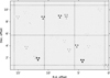 |
Fig. 1 Example of a section of a triple-exposure image. The figure shows an example of overlapping stellar triplets and a triplet hitting a réseau grid. |
2.1 Astrometric fitting
All the astrometric fits of the plates were based on using reference stars from DR2. We did not redo the fits with EDR3-based reference stars because tests indicated that there would be very limited gain, and this would clearly not outweigh the significant amount of work (there are many plates that would require manual tuning of the fitting parameters). We studied the difference between DR2- and EDR3-based astrometry by fitting astrometry for some plates by using astrometric reference stars from EDR3. By comparing the coordinates of the CduC stars we found that the coordinate differences between DR2- and EDR3-based astrometric fits are insignificant for us. This was as expected because the stars used for astrometric fitting are bright at Gaia’s scale, and astrometric fitting is a least-square procedure, which is not sensitive to small random coordinate shifts of reference stars. However, we performed the cross-match between the CduC and Gaia sources both for DR2 and EDR3 data. We made the magnitude equation correction separately for DR2- and EDR3-based coordinates.
In the following, we present the search and analysis of nonsingle-star candidates based on EDR3 data. Furthermore, in the appendix we give a description of the results based on DR2 data.
2.2 Magnitude equation correction
The celestial coordinates given by SCAMP have to be corrected for the effects of the so-called magnitude equation. It is caused by the combined effect of asymmetric stellar profiles (due to aberration in our case) and the non-linear response of the plate emulsion. The magnitude equation induces magnitudedependent shifts to the stellar coordinates. Based on the shape of the stellar profiles on the CduC plates, we expect that the magnitude of the coordinate shift is greatest at the plate edges, with the shift being radial from the plate centre.
Here we used a matching distance of 3 RMSastr between the CduC and Gaia sources, and the GBP magnitude of the Gaia stars was limited to values <16.5 mag and <16 mag, for the single-and triple-exposure plates, respectively. We divided the plate area (~2 × 2°) into 20 × 20 square bins, each with a size of ~0.1 × 0.1°. Within each bin, we derived the mean values of the coordinate differences between CduC and Gaia, separately along RA and Dec, using iterative 3-σ clipping. Then, the 20 × 20 maps were smoothed with a Gaussian kernel having σ = 0.1°. An example is shown in Fig. 2. The coordinate differences along RA and Dec show a rather complicated structure (panels a and b), but the coordinate difference vectors (panel d) point radially outwards and are greatest at the plate edges, as expected. Here, the coordinate differences are defined as Gaia minus CduC coordinates.
The vector flow representations of the effect of magnitude equation in different magnitude intervals, for single- and tripleexposure plates, are shown in Figs. 3 and 4, respectively. The magnitude ranges were chosen so that changes in the vectors were properly followed. The vector flows were consistent between single- and triple-exposure plates. For the brightest magnitude ranges, the vectors were radially outwards, while for the dimmest magnitude ranges, the vectors were radially inwards. For magnitude ranges in between, the behaviour of the vectors was more complicated.
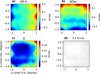 |
Fig. 2 Example of the derivation of magnitude equation correction for single-exposure stars within the GBP magnitude range 10.6–11.1 mag. In all panels, the plate area is shown as divided into 20 × 20 bins. Panel a) shows the mean value of the differences between the CduC and Gaia coordinates, along RA (ΔRA). Panel b) shows the mean value of the differences between the CduC and Gaia coordinates, along Dec (ΔDec). Panel c) shows the magnitude of the coordinate differences ( |

3 Results
The total number of plates included in our study was 986, out of which 572 were single-exposure plates and 414 were tripleexposure plates. This is 22 fewer than the number of the original plates of the Helsinki survey, 1008. Some of the plates were missing, while some were of too low quality.
Figure 5 shows the coordinate uncertainties related purely to the source extraction on the CduC plates. In the case of the single-exposure plates, the uncertainty is that given by SExtractor. In the case of the triple-exposure plates, the uncertainty is that given by our procedure fitting three Gaussian functions to the star triplets. Also plotted are the histograms of the coordinate uncertainties for the Gaia DR2 and EDR3 stars at the epoch of the plates. In all cases, the histograms are indistinguishable along RA and Dec.
The distortions in our images were caused by the telescope (optics, possible misalignment of the plate holder, and possible deformation of an emulsion) and our imaging system (camera detector, lens, and a possible misalignment of the plate on the light table). To find out the dominating source of distortions, we took two images of a plate, with a 90° rotation of a plate between the images. If the distortion maps produced by SCAMP were similar in the RA and Dec coordinate system, the dominating source of the distortions was the telescope. If the distortion maps were similar in the camera’s pixel coordinate system, the dominating source of the distortions was our imaging system. We find that the dominating source was our imaging system. Whatever the unknown distortions caused by the telescope were, they were either insignificant or they were fitted together with the distortions of our imaging system because the astrometric residuals as a function of pixel coordinates did not show large-scale variations.
The histograms of the RMS uncertainties of the astrometric fits, given by SCAMP, are shown in Fig. 6, separately. for the single- and triple-exposure plates. The histograms are given separately for the stars that have a S/N > 10 and a S/N > 70 (‘all stars’ and ‘high S/N stars’ in the SCAMP nomenclature) in the single-exposure plates, and a S/N > 5 and a S/N > 50 in the triple-exposure plates. The RMS uncertainties are about equal along RA and Dec, with a value of RMS = 0.14 ± 0.05″, and RMS = 0.12 ± 0.04″, in the single- and triple-exposure plates, respectively, for the high S/N stars.
After applying the magnitude-equation correction (Sect. 2.2), the mean value of the Δ(CduC-Gaia) coordinate differences are zero within the magnitude and coordinate bins shown in Figs. 3 and 4. Figures 7 and 8 show standard deviations of the Δ(CduC-Gaia) coordinate differences ( ) within the same magnitude and coordinate bins. The increase in deviation is only a function of a distance of a star from the centre of a plate. The radial increase in deviation is most prominent for weaker magnitudes, GBP ≳ 12 mag, where the deviation is rather constant up to distances ~0.7° from the plate centre, after which it increases to a value ~0.2″ near the corners of a plate.
The scatter plots for the differences between the CduC and Gaia coordinates (that is, between fitted and predicted coordinates) along RA and Dec are shown in Figs. 9 and 10 for the single- and triple-exposure plates, respectively. The distributions of the coordinate differences are expected to be normal, that is, the probability distribution would be Gaussian. However, the distributions have clearly non-Gaussian wings. The sources in the wings are sources whose pixel coordinates at the plate or the proper motion values in the Gaia DR2 catalogue are incorrect due to one of the following reasons: (i) the image of the source on a CduC plate is faulty, and thus the CduC coordinates are spurious; (ii) there are nearby sources, either physically connected or not, which are resolved by Gaia, but not by CduC, and thus the CduC coordinates are not meaningful and source matching between CduC and Gaia is wrong; (iii) the source is a double or multiple source that is not resolved or only occasionally resolved by Gaia; and (iv) there are astrometric calibration uncertainties in the Gaia data.
We used the empirical Moffat function to fit the distributions of the coordinate differences, because it can perfectly fit both the core and the wings of the distributions. The Moffat function has the form
 (1)
(1)
where σ is a width parameter. The fitted values of σMoffat are σMoffat ≈ 0.14″ and σMoffat ≈ 0.11″, in the single- and tripleexposure plates, respectively. We also fitted the histograms with a Gaussian function by limiting the fit to the core of the distributions, within the range [−0.1″,0.1″]. The fitted values of the width were σGauss ≈ 0.09″ and σGauss ≈ 0.07″, in the single- and triple-exposure plates, respectively. We believe that σGauss gives the true accuracy of the astrometry.
Figures 11 and 12 show the coordinate differences between CduC and Gaia as a function of Gaia GBP magnitude, for the single-exposure and triple-exposure plates, respectively. It is evident that, for weak magnitudes, GBP ≳ 13 mag, the coordinates are more accurate in the triple-exposure plates. We define the completeness limit of our CduC survey as the turning point of the histogram of the number of stars within magnitudes bins, as shown in Figs. 11 and 12 with solid white lines. The completeness limits at single- and triple-exposure plates are ~14.1 mag and ~13.6 mag, respectively. We define the limiting magnitude of our CduC survey as the point where the cumulative number of stars reaches 99% of the total number of stars, as shown in Figs. 11 and 12 with dashed white lines. The limiting magnitudes at single- and triple-exposure plates are ~15.5 mag and ~14.9 mag, respectively.
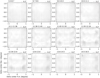 |
Fig. 3 Vector flow representation of the effect of the magnitude equation, for all the single-exposure plates, at different GBP magnitude ranges. At the top of each panel, the magnitude range is given and a vector with a length of 0.2″ is shown. |
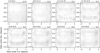 |
Fig. 4 Vector flow representation of the effect of magnitude equation, for all the triple-exposure plates, at different GBP magnitude ranges. At the top of each panel, the magnitude range is given and a vector with a length of 0.2″ is shown. |
 |
Fig. 5 Normed histograms for the coordinate uncertainties of stars, including only the uncertainties related to epoch transformation (Gaia) or source extraction (CduC). The histograms are indistinguishable both along RA and Dec. The red line is for the coordinate uncertainties in the single-exposure plates, as given by SExtractor. The green line is for the coordinate uncertainties in the triple-exposure plates, as given by our fitting procedure. The blue and orange lines are for the coordinate uncertainties of the Gaia DR2 and EDR3 stars at the epoch of the plates, respectively. The vertical black line gives one-tenth of the pixel size of our digital images. |
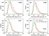 |
Fig. 6 Astrometric RMS values given by SCAMP for the singleexposure plates (panels a and b) and triple-exposure plates (panels c and d), separately along RA and Dec. For the single-exposure plates, the red histograms are for the stars that have S/N > 10, and the green histograms are for the stars that have S/N > 70. For the triple-exposure plates, the red histograms are for the stars that have S/N > 5, and the green histograms are for the stars that have S/N > 50. |
3.1 Error budget of astrometric fits
The RMS uncertainty of an astrometric fit, as given by SCAMP, includes contributions from four sources: (i) the uncertainty of the pixel coordinates of the stars; (ii) the uncertainty of the predicted stellar coordinates at the epoch of a plate, due to the imperfect proper motion values given by Gaia; (iii) the magnitude equation; and (iv) the imperfect fit of the image distortions. The combined effect of the sources (i) and (iv) above can be estimated by taking several images of a single plate, each image taken at a different position of a plate and also rotating the plate by multiples of 90° (the grid lines have to stay vertical and horizontal), then fitting astrometry to each image, and calculating the deviations of the RA and Dec coordinates of each star. The contributions of the sources ii) and iii) above are constant for each star and can be neglected when working with multiple images of a single plate. This analysis was done for the single-exposure plate #886 and the triple-exposure plate #882 because they have one of the largest number of stars per plate. For both plates, the deviations of coordinates were calculated for stars that were imaged between four and 52 times. The histograms of the deviations of the coordinates are shown in Fig. 13. The distributions of the standard deviation along the RA and Dec coordinates in the single-exposure plate peak at ~0.035″, although the whole distribution along RA is shifted to slightly larger values than along Dec. In the triple-exposure plate, the distributions peak at ~0.02″ along Dec and ~0.03″ along RA. These distributions could be explained by the fact that tracking errors, which are solely along RA, produce slightly elongated stellar profiles along RA. Thus, the pixel coordinate uncertainties are slightly larger along RA. This effect is more pronounced in the triple-exposure plates where the pixel coordinates of stars are more accurate than in the single-exposure plates because the coordinates are mean values over the stellar triplet. But in practice, the largest amount of elongation is caused by aberration, which mostly elongates the stars radially relative to the centre of a plate.
The deviations are comparable to the uncertainties related to source extraction only (Fig. 5). We thus conclude that, for a single plate, the contribution of an imperfect fit of the image distortions to the total uncertainty of an astrometric fit is not significant. This is in agreement with the fact that the Δ(CduC-Gaia) coordinate difference as a function of the x or y pixel coordinates of a plate does not show smooth, large-scale variations, which would be a sign of an imperfect fit of the image distortions.
In our standard analysis, the astrometric fit was derived in eight sub-regions for each plate. The mean value of the astrometric RMS along RA and Dec over these eight regions was 0.12 ± 0.02″ both for the plate #886 and #882. We thus estimate that the uncertainty associated with the pixel coordinates of the stars contributes less to the total uncertainty of the astrometric fits than uncertainties coming from the sources ii) and iii) above.
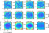 |
Fig. 7 Standard deviation of the Δ(CduC-Gaia) coordinate differences for the single-exposure plates. The data are given in the same coordinate and magnitude bins as in Fig. 3. |
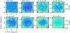 |
Fig. 8 Standard deviation of the Δ(CduC-Gaia) coordinate differences for the triple-exposure plates. The data are given in the same coordinate and magnitude bins as in Fig. 4. |
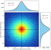 |
Fig. 9 Scatter plot for the coordinate differences between CduC and Gaia EDR3, for the single-exposure plates. The plot is limited to values between [−0.5″, 0.5″]. The histograms show the distributions along RA and Dec. The black line shows a fitted Moffat function. The solid red line shows a Gaussian function fitted to the core of the distribution, while the dashed red line shows the Gaussian function outside the core used for the fit. The widths of the Moffat and Gaussian functions are given. |
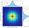 |
Fig. 10 Scatter plot for the coordinate differences between CduC and Gaia EDR3, for the triple-exposure plates. The plot is limited to values between [−0.5″, 0.5″]. The histograms show the distributions along RA and Dec. The black line shows a fitted Moffat function. The solid red line shows a Gaussian function fitted to the core of the distribution, while the dashed red line shows the Gaussian function outside the core used for the fit. The widths of the Moffat and Gaussian functions are given. |
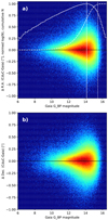 |
Fig. 11 Coordinate differences between CduC and Gaia EDR3 as a function of Gaia GBP magnitude, for the single-exposure plates. Panel a) is for RA and panel b) is for Dec. The normed histogram of the logarithm of the number of stars within the magnitude bins is shown as a solid white curve, and the completeness magnitude limit of the CduC survey is shown as a vertical solid white line. The normed cumulative number of stars is shown as a dashed white line, and the 99% magnitude limit is shown as a vertical dashed white line. |
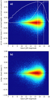 |
Fig. 12 Coordinate differences between CduC and Gaia EDR3 as a function of Gaia GBP magnitude, for the triple-exposure plates. Panel a) is for RA and panel b) is for Dec. The normed histogram of the logarithm of the number of stars within the magnitude bins is shown as a solid white curve, and the completeness magnitude limit of the CduC survey is shown as a vertical solid white line. The normed cumulative number of stars is shown as a dashed white line, and the 99% magnitude limit is shown as a vertical dashed white line. |
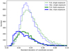 |
Fig. 13 Histograms of the standard deviations of RA and Dec coordinates of stars, after imaging a single plate several times, fitting astrometry to each image, and deriving standard deviations of the coordinates for each star. The data sample includes stars that have been imaged from four to 52 times. The histogram plotted with a thin line is for the single-exposure plate #886, the histogram plotted with a thick line is for the triple-exposure plate #882. |
3.2 CduC source catalogues
We give two sets of source catalogues, separately for single-and triple-exposure plates: (i) catalogues that include all the sources detected on the plates; and (ii) catalogues that include the sources that have been cross-match with the Gaia DR2 and EDR3 sources, at the epoch of each plate.
- (i)
These catalogues should not be used without visual inspection of sources, especially because the sources on the single-exposure plates can be false detections. In the triple-exposure plates, there is a much smaller probability of a false detection because a source detection requires a triplet of sources. We give the mean value of the coordinates for those CduC sources that appeared twice or more in the overlapping images of a certain plate. The coordinates are given at the epoch of each plate.
- (ii)
Because our aim was to find stars that have CduC coordinates deviating from the expected ones, we set the matching distance to 40 RMSastr, and the GBP magnitude limit of the Gaia stars to the limiting magnitude of the single- or triple-exposure plates (15.5 mag and 14.9 mag). We give a mean value of the coordinates for those CduC stars that appeared twice or more on the overlapping images of a certain plate. The catalogue for single-exposure plates contains ~831 000 Gaia sources, out of which ~749 000 are unique. The catalogue for triple-exposure plates contains ~325 000 Gaia sources, out of which ~302000 are unique. About 79% of the Gaia sources in the triple-exposure plates were also in the single-exposure plates. In theory, this percentage is expected to be 100%, because the areas covered by the triple-exposure plates are fully covered by the single-exposure plates, and the triple-exposure plates have a brighter limiting magnitude. The reasons for this discrepancy are: (i) the réseau grids of the single- and triple-exposure plates are not at the same positions on the sky, and (ii) there are areas on the sky where the limiting magnitude of a triple-exposure plate is actually dimmer than that of a single-exposure plate.
The area of the CduC Helsinki survey is about 2106 square degrees. The expected number of stars on the single-exposure plates was derived by selecting from the Gaia EDR3 catalogue the stars within the coordinate range of the Helsinki survey, and limiting the magnitudes to GBP < 13 mag, that is, over the region where the logarithm of the number of the CduC stars increases linearly as a function of magnitude (see Fig. 11). The number of such stars is ~254 000, while we detected ~211 000 singleexposure stars within the same magnitude limit, about 83% of the expected number. This discrepancy can be partly explained by the réseau grids. They occupy ~6% of the plate areas, but the effective area of the grid lines is larger because stars are not point sources. By using a typical radius of a star on our digital images, 4.3 pixels, the effective area is ~10% of the plate areas. Furthermore, there are abrupt changes in stellar densities between some adjacent plates. This implies that some of the plates were taken in less than optimal weather conditions, reducing the number of detected stars.
The number of triple-exposure stars is clearly less than the number of single-exposure stars because: (i) the star triplets are more easily disturbed by the réseau grids than the single stars; (ii) the star triplets overlap other star triplets, especially in areas of high stellar surface density; (iii) the triplets of the brightest stars are merged into single blobs, which are not identified as valid stars in our analysis; (iv) the single-exposure plates cover four declination values, while the triple-exposure plates cover only three values; and (v) the limiting magnitude of the triple-exposure plates is ~0.6 mag lower due to their shorter exposure time.
3.3 Non-single-star candidates in the Gaia EDR3 data
The candidates for non-single stars are stars for which there is a significant difference between the CduC and Gaia coordinates, at the epoch of a plate. A visual inspection of such stars reveals that many of them are weak, their stellar profiles are bad, or the stellar triplets are overlapping. Therefore, to find reliable candidates of non-single stars we limited the search to magnitudes GBP < 13 mag, and used the following two methods: (i) a ‘visual’ method, based on visual selection of stars that have error-free images both on a single- and triple-exposure plate. This was done only for Gaia DR2 data, and the results are given in the appendix. We did not redo this analysis with Gaia EDR3 data because that would have required too much manual work; (ii) a ‘correlation’ method, based on a correlation of the Δ(CduC-Gaia) coordinate differences between single- and triple-exposure plates. Because the single- and triple-exposure plates overlap, good candidates for non-single stars are stars for which the differences between the CduC and Gaia coordinates are significant and similar both in a single- and a triple-exposure plate. It is unlikely that a Δ(CduC-Gaia) coordinate difference would be similarly false on a single- and triple-exposure plate. Here we assumed that the epoch difference between a single- and triple-exposure plate of the same sky position was negligible compared to the epoch difference between the CduC and Gaia surveys. This analysis was done both for the Gaia DR2 and EDR3 data, but the results for the DR2 data are given only in the appendix.
Figure 14 shows scatter plots for the Δ(CduC-Gaia) coordinate differences between the single- and triple-exposure plates. The GBP magnitude of the sources were limited to <13 mag, and the distances of the sources from the plate centre were limited to <0.95°. The star-shaped distribution is a natural consequence of the plate overlapping; the corners of the plates, where astrometry has the largest scatter (that is, most affected by elongated stellar profiles), are located at the centres of the adjacent plates, where the astrometry has the smallest scatter. For example, in Fig. 14a the stars that have a large scatter along the x-axis and a small scatter along the y-axis are located near the edge of a singleexposure plate, but on a triple-exposure plate, they are located between the centre and the edge.
For the sources shown in Fig. 14, the ‘correlation’ method was executed in the following way: i) we took those sources for which the total difference between the positions in single- and triple-exposure plates was less than 3σ (we assumed that the 1σ uncertainty of the coordinates of stars was 0.09″ see Sect. 3); ii) the Δ(CduC-Gaia) coordinate differences along RA and Dec were derived as mean values of the corresponding differences in the single- and triple-exposure data.
We then selected three samples of stars: (i) stars for which the Δ(CduC-Gaia) coordinate difference was >0.4″, called sample S4; the number of stars was 1012; (ii) stars for which the Δ(CduC-Gaia) coordinate difference was between 0.25″–0.4″, called sample S3; the number of stars was 3092; (iii) a sample of stars for which the Δ(CduC-Gaia) coordinate difference was <0.1″, called sample S1. Samples S4 and S3 were candidates of non-single stars.
It was expected that a certain number of the CduC stars were binary stars, either physical or visual binaries, which were seen as a single star on a CduC plate, but were seen as separate stars by Gaia. Thus, we excluded the stars for which the second nearest star in the Gaia catalogue, at the epoch of the plate, was at a distance of <10″ and with a magnitude GBP < 15.5 mag (the 99% completeness limit of the single-exposure plates). The percentage of stars with a close companion star in samples S1, S3, and S4 was about 0.01%, 15%, and 49%, respectively.
The scatter plots for the Δ(CduC-Gaia) coordinate differences between single- and triple-exposure plates for sample S4 are shown in Fig. 15. There is no correlation between the Δ(CduC-Gaia) coordinate difference and the RMS value of the astrometric fit made by SCAMP, or between the coordinate difference and the error of the value of the proper motion.
Figure 16 shows, for the three CduC samples above, the histograms of the following Gaia EDR3 parameters: ruwe (Gaia renormalised unit weight error), parallax, parallax error, proper motion error, astrometric_excess_noise (the disagreement, expressed as an angle, between the observations of a source and the best-fitting standard astrometric model), astrometric_excess_noise_sig (significance of excess noise), error of the RA and Dec coordinates at epoch J2016.0, visibility_periods_used (number of visibility periods used in astrometric solution), astrometric_n_bad_obs_al/astrometric_n_good_obs_al (number of bad AL (along-scan) observations divided by number of good AL observations), astrometric_sigma5d_max (the longest semi-major axis of the 5-day error ellipsoid), ipd_gof_harmonic_amplitude (a large value indicates that the source is double), ipd_frac_multi_peak (fraction of observation windows indicating that the detection may be a resolved double star, either an optical pair or a physical binary), and ipd_frac_odd_win (a high value indicates that a source is disturbed by nearby sources in a crowded field or due to a nearby bright (G < 13 mag) source). In Fig. 16, the number of sources is equal in each sample.
For sample S1, the ruwe values are highly concentrated to values around one, while, in samples S3 and S4, the ruwe values extend to much higher values, indicating that there are stars that are problematic for Gaia’s astrometric solution. The values of parallax in sample S1 are strictly limited to values >0, while the values in samples S3 and S4 extend also to negative values. Furthermore, samples S3 and S4 have a larger proportion of large parallax values. All the Gaia parameters, except visibility_periods_used, indicate an increasingly lower quality for Gaia’s single-star astrometric fit when going from sample S1 to samples S3 and S4. The parameter ipd_frac_odd_win is highly concentrated on a value of zero for all the samples, indicating that our removal of nearby sources (Sect. 3.3) is working well.
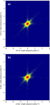 |
Fig. 14 Correlations of the Δ(CduC-Gaia) coordinate differences between single- and triple-exposure plates for Gaia EDR3 data. Panel a) is along RA and panel b) is along Dec. This figure is limited to sources with magnitudes GBP < 13 mag, and with distances from the plate centre to <0.95°. |
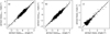 |
Fig. 15 Correlations of the Δ(CduC-Gaia) coordinate differences between single- and triple-exposure plates for non-single-star candidates. The candidates are the EDR3-based sources in the ‘correlation’ S4 sample, that is, sources for which the Δ(CduC-Gaia) coordinate difference is >0.4″ (Sect. 3.3). Panels a, b, and c show the correlations for RA coordinate difference, Dec coordinate difference, and total coordinate difference, respectively. The straight lines show a one-to-one correlation. |
3.4 Gaia’s astrometric quality indicators
The Gaia catalogues include several indicators of astrometric quality of a Gaia source (Lindegren 2018). The different indicators give different information: the sources with the most ‘precise’ astrometric data can be selected based on the formal uncertainties of the relevant parameters (e.g. parallax error); the sources with the most ‘reliable’ astrometric data can be selected based on the parameter visibility_periods_used (a higher number means less sensitivity to bad measurements); the sources whose observations are ‘consistent’ or ‘inconsistent’ with the astrometric five-parameter model can be selected based on the unit weight error (UWE) or, preferably, the ruwe parameter. Overall, the recommended quality indicator is ruwe. It has been shown that ruwe is sensitive to unresolved companions, and to the motion of the photocentre of unresolved binaries themselves (Belokurov et al. 2020; Stassun & Torres 2021). Figure 16 shows histograms for these and several other Gaia EDR3 parameters measuring the goodness of a single-star astrometric fit. In addition to the ruwe, the astrometric_excess_noise is sensitive to the photocentric motions of unresolved objects, such as astrometric binaries. The following values of the parameters indicate that a source is astrometrically well behaved; ruwe≈ 1; astrometric_excess_noise=0; astrometric_excess_noise_sig≲ 2. However, because our S1 sample was assumed to consist of single stars, the S1 sample could be used to derive limits for Gaia parameters that indicate whether a star is or is not astrometrically well behaved. We derived these limits by calculating 95% quantiles for the S1 sample. If the value of a Gaia parameter was greater than the value of the 95% quantile of the S1 sample, the star is astrometrically ill-behaved. The derived limits for Gaia parameters are shown in Table 1, together with the percentage of such sources in our samples of non-single-star candidates that have a Gaia parameter value greater than the limit.
In Table 1, the following Gaia parameters are the most efficient ones to classify the stars in sample S4 as nonsingle-star candidates: ruwe, parallax_error, proper motion error, astrometric_excess_noise, astrometric_excess_noise_sig, RA/Dec error, and astrometric_sigma5d_max. About 40% of the stars in sample S4 have values for these Gaia parameters that are consistent with the values derived for the sample of single-star candidates (sample S1).
For our purposes, the most interesting stars are those that have a good astrometric fit indicated by ruwe, or by any other quality indicator of Gaia, although the Δ(CduC-Gaia) coordinate difference is significant. A possible explanation for the discrepancy between the derived and expected coordinates is that we have a wrong cross-match between the CduC and Gaia source, because the correct Gaia star is a variable star that was too dim to be detected on a CduC plate at the epoch of the observations. To test this hypothesis, we performed a cross-match between the CduC sources in sample S4 and the Gaia sources, at the epoch of the plates, without magnitude limitations for the Gaia sources. We find that for about 6% of the CduC sources, there is another Gaia source that is closer to the CduC source than the one found in our original analysis. However, for these sources the Gaia EDR3 catalogue does not give the GBP magnitudes, while our analysis used only sources for which the GBP magnitude is available. Thus, about 6% of our non-single-star candidates in sample S4 are close double stars, resolved by Gaia, for which the GBP magnitude is available only for the other source. We conclude that a cross-match of a CduC source in sample S4 with a variable Gaia source is not probable. We infer that the sources that are classified as non-single-star candidates by us, although Gaia makes a good single-star astrometric fit for them, are long-period binary stars, with periods of the order of 100 yr. Around this period Gaia has a minimum in the detection efficiency of double stars.
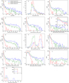 |
Fig. 16 Histograms of Gaia EDR3 parameters for samples S1, S3, and S4, based on the ‘correlation’ method (Sect. 3.3 ii)). The plotted histograms contain an equal number of sources from each sample. The red, green, and blue histograms are for stars for which the Δ(CduC-Gaia) coordinate distance is <0.1″, between [0.25, 0.4]″, and >0.4″, respectively. The Gaia parameters are ruwe (a), parallax (b), parallax error (c), proper motion error (d), astrometric_excess_noise (the disagreement, expressed as an angle, between the observations of a source and the best-fitting standard astrometric model (e)), astrometric_excess_noise_sig (significance of excess noise (f)), error of RA and Dec coordinates at epoch J2016 (g), visibility_periods_used (number of visibility periods used in astrometric solution (h)), astrometric_n_bad_obs_al/astrometric_n_good_obs_al (the number of the bad AL (along-scan) observations divided by the number of the good AL observations (i)), astrometric_sigma5d_max (the longest semi-major axis of the 5-day error ellipsoid (j)), ipd_gof_harmonic_amplitude (a large value indicates that the source is double (k)), ipd_frac_multi_peak (fraction of observation windows indicating that the detection may be a resolved double star, either an optical pair or a physical binary (l)), and ipd_frac_odd_win (a high value indicates that a source is disturbed by nearby sources in a crowded field or due to a nearby bright (G < 13 mag) source (m)). The histograms of proper motion error (d) and RA and Dec coordinate error (i) include errors along RA and Dec separately, and thus they have lower noise than the other histograms. |
Classification of stars into single- and non-single-star candidates.
3.5 Improved astrometry with multiple imaging
For weaker magnitudes, GBP ≳ 13 mag, the astrometric accuracy is worsened by low accuracy of the pixel coordinates of stars, especially for the single-exposure plates (Fig. 11). Because it is fast to take numerous images with a digital camera, it is worthwhile studying whether astrometric accuracy of these stars can be improved by taking several images of a single plate, with each image taken at a different position, fitting astrometry to each image, and deriving mean values of RA and Dec coordinates. This analysis was done by using the same multiple imaging data as in Sect. 3.1.
Figure 17 shows the Δ(CduC-Gaia) coordinate differences of stars, as derived both with standard and multiple imaging. Panel a) includes all the stars for which the coordinate difference in standard imaging is greater than 0.4″, and which have a magnitude GBP > 13 mag. Panel b) includes all the stars for which the coordinate difference in standard imaging is greater than 0.3″, and which have a magnitude GBP < 13 mag. For plate #886, a coordinate difference of 0.1″ corresponds to about 1 RMSastr. The two data points of each star (standard and multiple imaging) are connected with a line. In panel a), for most of the stars, the effect of multiple imaging is to move the data points radially towards a (0,0) coordinate difference, that is, multiple imaging gives coordinates that are closer to the correct ones. About 58% of the stars are such that their distance from a (0,0) coordinate difference is >0.4″ in the case of standard imaging, but not in the case of multiple imaging. In panel b), the lines connecting the data points are shorter and their orientations are more random than in panel a).
We conclude that the gain obtained with multiple imaging is not significant for bright (GBP ≲ 13 mag) stars. However, for weaker stars multiple imaging can make a difference between classifying and not classifying a star as a non-single star. By extending the results obtained for plate #886 to the whole data, we estimate that, for example, if classifying all the stars with a magnitude GBP > 13 mag and with a Δ(CduC-Gaia) coordinate difference >4 RMSastr as non-single stars, about 58% of the stars are wrongly classified. Taking into account the extra work associated with multiple imaging, it is justified only if there is interest in particular stars with a magnitude GBP ≳ 13 mag.
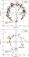 |
Fig. 17 Δ(CduC-Gaia) coordinate differences for standard and multiple imaging data for the single-exposure plate #886. In multiple imaging, the coordinates are mean values of coordinates derived over several images and astrometric fits. The red and green dots are for standard and multiple imaging, respectively. The lines connect the data points of each star. The data shown in panel a) is for stars that have the Δ(CduC-Gaia) coordinate difference in standard imaging greater than 0.4″ and that have a magnitude GBP > 13 mag. The circle has a radius of 0.4″. The data shown in panel b) is for stars that have the Δ(CduC-Gaia) coordinate difference in standard imaging greater than 0.3″ and that have a magnitude GBP < 13 mag. The circle has a radius of 0.3″. |
4 Comparison with other catalogues
4.1 Tycho Double Star Catalogue
The Tycho Double Star Catalogue (TDSC, Fabricius et al. 2002) contains 103259 double stars. We performed a crossmatch between TDSC and our non-single-star candidates in two steps: (i) a cross-match between Tycho sources and our candidates by using the catalogue gaiaedr3.tycho2tdsc_merge_best_neighbour at the Gaia archive; and (ii) using the catalogue gaiaedr3.tycho2tdsc_merge to check whether the Tycho source is listed in the TDSC. We find that, for the ‘correlation’ samples S1, S3, and S4, the percentage of sources listed in the TDSC is about 0.8%, 4% and 8%. However, in our data analysis we largely removed those binaries that would be in the TDSC. Our samples were free of the CduC sources for which the second-closest Gaia source was at a distance of <10″, and had a magnitude GBP < 15.5 mag. On the other hand, in the TDSC, the best conditions for separations of the components are between 1″–3″, and the magnitudes have values VT ≲ 12 mag (Fabricius et al. 2002). When we performed the cross-match between the TDSC and the CduC sources that were discarded from the ‘correlation’ S4 sample because for them the second-closest Gaia source was at a distance of <10″, we found that ~33% of the sources were in the TDSC.
In the case of the ‘correlation’ S4 sample, without discarding the sources for which the second-closest Gaia source is at a distance of <10″, the TDSC gives the separation of the binary components for 41 sources. There are 32 TDSC systems that have a component separation ⩽5.3″. We detected these sources because two close stars on a CduC plate make the stellar profiles faulty. The remaining nine systems have separations between about 28″–98″, and these sources were detected by us because their proper motion values given by Gaia are spurious.
4.2 SB9 catalogue of spectroscopic binaries
A cross-match of our candidates in the ‘correlation’ S4 sample with the sources in the SB9 catalogue (Pourbaix et al. 2004), which is a catalogue of spectroscopic binaries, gave only two matches. The periods of these sources are about 581 and 1862 days. On the other hand, if our analysis finds binary stars with periods of about 100 yr, as hypothesised in Sect. 1, the binaries may have orbital speeds too small to be measured spectroscopically.
4.3 Wide binaries from Gaia EDR3
The catalogue of El-Badry et al. (2021) is a compilation of about one million spatially resolved binary stars from Gaia EDR3. The catalogue includes binary stars with periods of up to about 108 yr, and with a separation up to ~1000″, while a histogram of separations has a maximum at ~2″. In the case of our ‘correlation’ S4 sample, about 26% of the sources are in the catalogue of El-Badry et al. (2021), if we do not discard those CduC sources that have a close companion source. If we discard them, about 11% of the sources are in the catalogue of El-Badry et al. (2021). In the case of the ‘correlation’ S3 sample, the corresponding percentages are about 10% and 7%. In the case of the ‘correlation’ S1 sample (i.e. single stars), the corresponding percentages are about 7% and 7%. These results provide evidence that most of our candidates of non-single stars are systems that are unresolved by Gaia. In addition, it is possible that some of our sources are hierarchical triples and higher-order multiples, which are missing in the catalogue of El-Badry et al. (2021) by a significant fraction.
4.4 The HIPPARCOS–Gaia Catalog of Accelerations
The HIPPARCOS–Gaia Catalog of Accelerations, HGCA, is a catalogue based on cross-calibration between HIPPARCOS and Gaia EDR3 data (Brandt 2021). This catalogue of 115,346 stars is suitable for identifying astrometrically accelerating systems. We took, from the HGCA catalogue, the sources that were accelerating at an equivalent significance of >3σ, that is, the χ2 value for a model of constant proper motion with 2 degrees of freedom was >11.8. The percentage of astrometrically accelerating sources in the ‘correlation’ S1, S3, and S4 samples are 0.3%, 1.2%, and 3.7%. Thus, most of the non-single-star candidates found by us do not have non-linear proper motions, if they are measured over the time span of HIPPARCOS and Gaia catalogues.
4.5 Companions of HIPPARCOS and Gaia EDR3 catalogue stars
Kervella et al. (2022) provide catalogues of proper-motion anomaly (PMa) and resolved common proper-motion (CPM) pairs. The PMa sources were detected by comparing the longterm (HIPPARCOS-Gaia) and short-term (solely HIPPARCOS or Gaia) proper motion vectors. The CPM catalogues include stellar pairs, both from the HIPPARCOS and Gaia catalogues, that have similar parallaxes and proper motion values. The comparison of the three catalogues given by Kervella et al. (2022) with our non-single-star candidates gives the following results. i) Catalogue of proper motion anomaly of HIPPARCOS stars. We selected the sources for which either the binary flag BinH2EG3a or BinH2EG3b (the proper motion anomaly between the longterm and either the HIPPARCOS or Gaia proper motions) was set to one. The percentages of sources in the ‘correlation’ samples S1, S3, and S4 that were in this catalogue were then ~0.2%, ~ 1.2%, and ~3.3%, respectively. ii) Catalogue of CPM candidate companions for HIPPARCOS stars. We selected the sources for which the ‘gravitationally bound candidate’ flag Bnd was set to one. The percentages of sources in the ‘correlation’ samples S1, S3, and S4 that were in this catalogue were then ~0.3%, ~0.2%, and ~0.8%, respectively. iii) Catalogue of CPM candidate companions for Gaia stars within 100 pc. We selected the sources for which the ‘gravitationally bound candidate’ flag Bnd was set to one. The percentages of sources in the ‘correlation’ samples S1, S3, and S4 that were in this catalogue were then ~0.4%, ~0.3%, and ~0.6%.
5 Discussion
The comparison of CduC and Gaia coordinates for our non-single-star candidates gives two undeniable facts: (i) the coordinate differences Δ(CduC-Gaia) are larger for those sources for which the uncertainties of Gaia’s astrometric fit are larger; and (ii) the coordinate differences are larger for DR2-based Gaia coordinates than for EDR3-based Gaia coordinates (see Appendix A.1). These facts can be explained in two ways: (i) the candidate stars are genuine non-single stars, for which Gaia’s single-star astrometric fits are spurious, and for which the EDR3-based values of proper motion better trace the common motion of a binary star; and (ii) the candidate stars are single stars that have biased proper motions due to astrophysical or instrumental effects, and the EDR3-based astrometry is more reliable than the DR2-based astrometry. For a discussion about the astrometric quality of the Gaia EDR3 and DR3 catalogues, see Fabricius et al. (2021) and Babusiaux et al. (2023), respectively. With the data currently available, we cannot say which one is the correct explanation for a particular source, unless the source has been identified as a non-single source also in some other study. In the next two paragraphs, we discuss both of these explanations in detail.
Firstly, we assume that the sources with a significant coordinate difference Δ(CduC-Gaia) are genuine binary stars, which are either unresolved or only occasionally resolved by Gaia. We then give the following items to show a consistency between this assumption and our results. (1) The movement of the photocentre of a binary star in a non-linear way on the plane of the sky adds noise to Gaia’s astrometric fit, which is made under the assumption of a single star moving linearly on the sky. (2) The following factors affect the movement of the photocentre: (i) orbital period of the binary star. A shorter orbital period means a faster movement of the photocentre; (ii) a change in the luminosity ratio of the components of a binary star. As a result, the photocentre shows an astrometric shift. These binary stars are called variability-induced movers (VIMs, Wielen 1996); (iii) the scan direction of Gaia. It is important for an individual transit measurement, but when averaging this over many dozens of different transits, dependencies are effectively washed out, and so this is not directly visible in the published Gaia data. (3) We find that, in general, the larger the coordinate difference Δ(CduC-Gaia), the larger the noise is in Gaia’s single-star astrometric fit, as indicated by almost all the quality indicators given in the Gaia catalogues. (4) Comparison with external catalogues of non-single stars shows that the larger the coordinate difference Δ(CduC-Gaia), the larger the percentage is of known non-single stars in our samples of non-single-star candidates. However, these percentages are relatively low, about 10% at maximum. (5) Figure A.1 shows that in the case of our samples of nonsingle-star candidates, the EDR3-based coordinates agree better, in general, with the CduC coordinates than the DR2-based coordinates. Because the EDR3 data spans over a longer time interval than the DR2 data, the proper motion values in EDR3 better follow the common motion of a binary or multiple star, which is the motion we are measuring from the CduC plates. (6) We used the astrometry spread function (ASF) method to derive the uncertainties of parallax, proper motion, and position that Gaia would observe for a simple point source. The ASF-based uncertainties are smaller than those given in the Gaia DR2 catalogue for our samples of non-single-star candidates (see Appendix A.2).
Secondly, we assume that the sources with a significant coordinate difference Δ(CduC-Gaia) are single stars. Thus, if the values of the proper motions are biased by some effect, then the position of a source, extrapolated to the epoch of the CduC observation, is also biased. There are also effects that can bias the values of astrometric errors. We list the following instrumental and astrophysical effects. (1) There can be errors in the observation-to-source matching. This is only occasionally challenging in high-density fields, or when close companions are present that are resolved by Gaia on some transits and unresolved on others. (2) There are red giant variable stars, such as Mira stars, which have a changing colour and magnitude. This may induce an apparent position change as seen by Gaia, because the colour-dependent model of the point spread function of the instrument currently assumes a constant colour for the astrometric solution. This then leads to biased values of proper motions. (3) In rare cases, bright sources (GBP ≲ 12 mag) may be observed with two (or even more exceptionally, three) different time-delayed integration (TDI) gates, varying from transit to transit. Each TDI gate has its own geometric calibration in the Astrometric Global Iterative Solution (AGIS), each of which has its own uncertainties. Astrometric solutions that combine transits observed with several gates can suffer from underestimated astrometric errors.
It is known that, at a magnitude of GBP ≲ 13 mag, Gaia’s astrometry is limited by calibration uncertainties (both in DR2 and EDR3), and these uncertainties are included in the errors of Gaia’s astrometric parameters. Thus, the observed coordinate difference Δ(CduC-Gaia) of each star can be compared with the errors of the CduC and Gaia coordinates. In the case of the CduC coordinates, we took the RMS value of the astrometric fit made for each sub-image as the error of the coordinates. In the case of the Gaia coordinates, the errors were the errors of the epoch-transformed coordinates of each star. In both cases, the errors were given separately along RA and Dec. Then, for each source we derived the expected error of the distance between the CduC and Gaia coordinates. In the case of the EDR3-based ‘correlation’ S4 sample, the mean value and standard deviation of the expected errors was 0.18 ± 0.06″. On the other hand, the mean value of the coordinate difference Δ(CduC-Gaia) was ~0.6″ for the same sample. Thus, the measured coordinate differences were deviant from zero at a ~3σ confidence level. However, it is known that the formal astrometric uncertainties of Gaia are underestimated in DR2 by 8–12% (Lindegren et al. 2018) or by ~10% (Arenou et al. 2018), and in EDR3 by 10%–20% (Vasiliev & Baumgardt 2021), by 22%±6% (Zinn 2021), by 10–70% (Maíz Apellániz et al. 2021), or by ~37% (Brandt 2021), and by a factor of up to two for uncertainty of parallax (El-Badry et al. 2021). It is clear that, at these levels, the underestimation cannot explain the coordinate differences. There can be other factors that affect the reliability of the formal uncertainties of the coordinates. For a single measurement of a star on a CduC plate, the factor could be a random, very local deformation of a plate emulsion that is not visible to the eye. However, we require that the coordinate differences Δ(CduC-Gaia) are similar both in the single- and triple-exposure plates, and it is very improbable that there would be a similar deformation in both of them. In general, the factor cannot be something that affects only the CduC coordinates in a random way, because that would not explain why the sources with a significant coordinate difference Δ(CduC-Gaia) also have a larger uncertainty for Gaia’s astrometric fit. We are confident that the CduC coordinates of our non-single-star candidates are reliable because they are similar on both the single- and tripleexposure plates. These facts support the assumption that the sources with a significant coordinate difference Δ(CduC-Gaia) are multiple sources for which Gaia’s proper motion values are spurious.
For the stars that have a significant coordinate difference Δ(CduC-Gaia) when using DR2-based data, the EDR3-based coordinates agree better with the CduC coordinates than the DR2-based coordinates (see Appendix A.1). Under the assumption that these stars are multiple stars, this can be explained by assuming that the proper motion values in EDR3 better follow the centre of mass of a binary or multiple star, which is the motion we measure from the CduC plates. However, there are two other phenomena that can be full or partial explanations: (i) the uncertainties of the proper motion values of all stars in the EDR3 data are lower due to normal error reduction caused by a longer time span of EDR3; and (ii) both for DR2 and EDR3, the astrometry of the bright stars (G ≲ 13 mag) is limited by calibration uncertainties, but these uncertainties are reduced in EDR3. Thus, the EDR3 astrometry has lower uncertainties. Looking at the stars shown in Fig. A.1, the mean values of the DR2-based and EDR3-based errors of proper motions are ~1.1 mas yr−1 and −0.21 mas yr−1, respectively. For an epoch transformation of coordinates over 100 yr, these errors would correspond to coordinate errors of ~0.1″ and ~0.02″, respectively, at the epoch of the plates. With these errors of coordinates, the mean value of the error of the distance between the DR2-based and EDR3-based coordinate differences Δ(CduC-Gaia) in Fig. A.1 c) is calculated to be −0.1″. However, the mean value of the observed coordinate shift is ~1.2″, a factor of about ten times larger. Thus, the decrease in the formal errors of the proper motion values when going from DR2 to EDR3 cannot be the explanation for the observed decrease in the coordinate difference Δ(CduC-Gaia) in Fig. A.1. If these stars are truly single stars, their astrometric solutions in DR2 may have been impacted by some of the astrophysical and/or instrumental effects discussed above, without being reflected in the formal errors of the proper motions.
For Gaia, the minimum angular separation between distinct sources depends on several factors, such as the magnitudes of the components of a close stellar pair and their relative orientation on the sky. In the case of EDR3, there are few close pairs with separations less than ~0.6″, while the separation is never less than 0.18″. An important astrometric limitation related to our study is that, for close pairs (e.g. at magnitude G ≃ 15 mag in EDR3), most neighbours at separation 0.18″−0.6″ have only a two-parameter solution (Lindegren et al. 2021). Thus, it is possible that our removal of close pairs, as done in Sect. 3.3, is not adequate because epoch transformation cannot be made for stars with only a two-parameter solution. However, we can estimate the significance of the close neighbours with only a two-parameter solution by rejecting from our samples of non-single-star candidates the stars for which the closest neighbour star satisfies the same criteria as used in Sect. 3.3, but at the epoch of the Gaia catalogues, without epoch transformation. We find that, in this way, the rejected number of stars increases by ~2%. Thus, the effect of neighbour stars with only a two-parameter solution is estimated to be insignificant for our study.
Our samples of non-single-star candidates include stars that have negative parallaxes (see Fig. 16). Negative parallaxes can be caused by a close (~0.2″−0.3″) alignment of sources, which are occasionally resolved by Gaia, depending on the scan direction. Most of these sources are faint sources on dense areas of the sky, and the negative parallax can be very far from zero with respect to the formal uncertainty of the parallax (Gaia Collaboration 2018). But our sources are bright on Gaia’s scale, they are not concentrated in the dense areas of the Galactic plane, and, for example, in the case of the ‘correlation’ S4 sample, the median of negative parallaxes extends only to about −1.4σ, where σ is the median value of parallax errors of negative parallaxes. Thus, we think that the negative parallaxes in our samples are mainly a result of error propagation in a noisy astrometric fit made by Gaia.
6 Conclusions
We present our ‘Carte du Ciel & Gaia’ project of digitising the Helsinki zone plate collection of the international Carte du Ciel survey. The CduC survey gives us a unique view of the sky as it was about 120 yr ago. With scientific dedication, the observational part of the CduC project of the Helsinki zone was completed more than a century ago. Now with Gaia data, it is finally possible to calibrate the data and to exploit them scientifically. With the Gaia Data Release 2 (DR2) and Early Data Release 3 (EDR3) data, we are, for the first time, in a situation where the proper motions of stars are accurate enough to calculate coordinates of stars, at the epoch of the CduC plates (~ 1900), with an uncertainty that is lower than the uncertainty related to source extraction on photographic plates.
We photographed the glass plates with a high-end commercial camera and calibrated the astrometry of the digitised images with the Gaia DR2 stars as astrometric reference stars. We show that, for the plates, typically 0.07″–0.09″ absolute astrometry can be achieved. We used the CduC data to identify sources that are not at the coordinates where they are expected to be on the CduC plates, based on the values and errors of proper motions, and present day coordinates derived by Gaia. These sources can be non-single, mostly binary stars, for which Gaia’s proper motion values are incorrect. These binaries are unresolved or occasionally resolved by Gaia, and thus Gaia observes the non-linear motion of the photocentre of the system. The nonlinear motion adds noise to Gaia’s astrometric fits, which are made under the assumption that the observed sources are single sources with a linear motion. The ASF method confirms that, for DR2-based data, the uncertainties of parallax, position, and proper motion of the non-single-star candidates are larger than those of a simple point source. We find that, in general, the further away a CduC source is from its expected position, at the epoch of the plate, the larger the uncertainties are of Gaia’s single-star astrometric fit, as indicated by several quality indicators of Gaia. We find that the differences between the expected and measured coordinates of the CduC sources are consistent on the partly overlapping single- and triple-exposure plates, that is, on two totally independent data sets. However, there are also other phenomena that can bias the values or errors of proper motions, such as the variability of Mira stars or errors in the observation-to-source matching. With the data currently available, we cannot exclude them as an explanation for the larger-than-expected difference between the CduC and Gaia coordinates.
The cross-matching between the CduC and Gaia sources was done by using Gaia sources both from DR2 and from EDR3, the latter of which spans over a longer time interval than DR2. By comparing the differences of the coordinate deviations Δ(CduC-Gaia) between DR2- and EDR3-based data, we find that for the majority of the DR2-based non-single-star candidates, the coordinate deviations become smaller when using EDR3-based Gaia data instead. The reason for this could be that EDR3, due to its longer observing period, has had more time to measure the common motion of stars in an unresolved binary system. The common motion is just the motion that we are measuring for binary stars on the CduC plates. Another explanation is that the number of stars with biased astrometric solutions is smaller in EDR3 data than in DR2 data, which is a known fact (Fabricius et al. 2021).
Acknowledgements
K.L. thanks the Jenny and Antti Wihuri foundation for financial support for this work. K.M.’s research supported by the Academy of Finland (grants 336546, 345115). This work has made use of data from the European Space Agency (ESA) mission Gaia (https://www. cosmos.esa.int/Gaia), processed by the Gaia Data Processing and Analysis Consortium (DPAC, https://www.cosmos.esa.int/web/Gaia/dpac/consortium). Funding for the DPAC has been provided by national institutions, in particular the institutions participating in the Gaia Multilateral Agreement. We acknowledge support from the ESTEC Faculty. We thank the anonymous referee for helpful comments.
Appendix A Non-single-star candidates in Gaia DR2 data
In the case of Gaia DR2 data, we searched for non-singlestar candidates by using two different methods: i) the ‘visual’ method, which was used only for DR2 data, and ii) the ‘correlation’ method, as has been described in Sect. 3.3 for EDR3 data. The starting point of the ‘visual’ method was the single-and triple-exposure star catalogues, which were made by using a search radius of 40 RMSastr between CduC and Gaia coordinates (RMSastr is the RMS value of each astrometric fit). From these catalogues, we selected the stars for which the Δ(CduC-Gaia) coordinate difference was >5 RMSastr on a triple-exposure plate, and the Gaia GBP magnitude was less than 13 mag. The limit of 5 RMSastr was chosen so as to not have too many sources for a laborious visual inspection. We then plotted both the single-and triple-exposure image of the star, regardless of the Δ(CduC-Gaia) coordinate difference on a single-exposure plate. If both the images were error free, the star was accepted for further analysis. The sources with a close Gaia companion star were then discarded, as was done in Sect. 3.3 in the case of EDR3 data. This method produced a sample of 484 CduC stars, hereafter called sample S5. Furthermore, we had two other samples, made in the same way as sample S5: i) a sample of 484 stars that had the Δ(CduC-Gaia) coordinate difference <1 RMSastr on a triple-exposure plate (hereafter sample S1), and ii) a sample of 484 stars that had the Δ(CduC-Gaia) coordinate difference between [2.5, 3.5] RMSastr on a triple-exposure plate (hereafter sample S3).
The ‘correlation’ method was applied for DR2-based data in exactly the same way as was done for EDR3-based data in Sect. 3.3. We built samples S1, S3, and S4, which included stars for which the Δ(CduC-Gaia) coordinate difference was <0.1″, 0.25″–0.4″, and >0.4″. The number of sources in samples S3 and S4 was 3286 and 2132.
Similarly to the Gaia EDR3-based data, the DR2-based data reveals that astrometric fits made by Gaia, made under the assumption that all the stars are single stars, are worse for our samples of non-single star candidates than for the samples of single stars. The histograms of Gaia DR2 parameters for the ‘visual’ and ‘correlation’ samples are similar to the histograms shown in Fig. 16 for the EDR3-based data. Table A.1 gives the percentages of such non-single-star candidates found by us, for which the quality indicators of Gaia’s astrometric fit, made under the assumption that sources are always single ones, indicate a bad fit. In the case of the ‘visual’ S5 and ‘correlation’ S4 samples, the percentages are up to about 90% and 80%, respectively. These values are higher than the corresponding percentage for the EDR3-based ‘correlation’ S4 sample, about 60% (see Table 1).
A.1 Comparison between Gaia DR2 and EDR3
We aimed to study whether the Δ(CduC-Gaia) coordinate differences can be smaller for EDR3 data than for DR2 data, as suggested in Sect. 1. The only factor changing the coordinate differences is a change in the proper motion values between DR2 and EDR3 (plus a change in Gaia coordinates between the epochs J2015.5 (DR2) and J2016.0 (EDR3), but that is insignificant for us). As a starting point, we took a sample of nonsingle-star candidates derived by using DR2 data. We then used the table gaiaedr3.dr2_neighbourhood in the Gaia archive to perform a cross-match between the source identifications given in the DR2 and EDR3 catalogues. Thus, the cross-match between CduC and Gaia coordinates was performed by using Gaia coordinates that were based on the proper motion values and epoch J2015.5 coordinates given in the DR2 data.
As a sample of non-single-star candidates, we took sample S4 of the ‘correlation’ method. For these stars, the DR2-based Δ(CduC-Gaia) coordinate difference was >0.4″. They are plotted in Fig. A.1 a. Then we plotted, for the same stars, the EDR3-based Δ(CduC-Gaia) coordinate differences as green circles in Fig. A.1 b. Then, about 64% of the stars were within a distance of 0.4″ from the origin. The movement of the Δ(CduC-Gaia) coordinate difference between DR2 and EDR3 data is shown in Fig. A.1 c, for the same data but for a sub-sample of 300 sources. The majority of the movements is radially towards the origin. It is evident that the coordinates of stars derived from the CduC plates agree better with the expected coordinates derived from EDR3 than with those derived from DR2. The results obtained do not have a dependence on the magnitude or the colour of stars.
Classification of stars into single and non-single-star candidates.
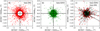 |
Fig. A.1 Comparison of the Δ(CduC-Gaia) coordinate differences between Gaia DR2 and EDR3. Panel a) shows the DR2-based Δ(CduC-Gaia) coordinate differences for the sources in sample S4 of the ‘correlation’ method, that is, sources for which the coordinate difference is >0.4″. The EDR3-based coordinate differences of the same stars are shown in panel b). Panel c) shows the DR2- and EDR3-based coordinate differences together, with a line connecting the two coordinate difference of each source. The sample shown in panel c) is a sub-sample of 300 sources out of the sources in panels a) and b). The circle in panels a) and b) has a radius of 0.4″. |
A.2 Astrometry Spread Function of Gaia DR2
We used the ASF to derive the expected uncertainties of astrometric parameters for the sources in samples S1, S3, and S4 of our ‘correlation’ method, under the assumption that they were single sources. The differences between the Gaia DR2based and ASF-based uncertainties are shown in Fig. A.2. For our non-single-star candidate samples S3 and S4, the observed uncertainties were larger than the expected ones, indicating that those sources have excess astrometric noise, and thus are not simple point sources.
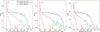 |
Fig. A.2 Differences in astrometric uncertainties between those given in the Gaia DR2 catalogue and those estimated by the ASF of Gaia DR2. Panel a) shows the differences in the uncertainties of RA and Dec coordinates (epoch J2015.5). Panel b) shows the differences in the uncertainties of proper motion along RA and Dec coordinates. Panel c) shows the differences in the uncertainties of parallax. Panels a) and b) separately include the values along RA and Dec coordinates, and thus the number of data points is twice that in panel c). The data consist of the S1, S3, and S4 samples of our ‘correlation’ method (Appendix A). |
Appendix B Catalogues of non-single-star candidates
We publish electronic tables of EDR3- and DR2-based candidates of non-single stars at the CDS/VizieR archive server (Tables 2-7). We list all the candidate stars found by our analysis, that is to say, we do not discard the stars that have a close companion. However, for each CduC star, we also identify the Gaia star that is second closest to the CduC star (at the epoch of a plate), and for these Gaia stars, we list their magnitude and distance from the CduC star. The search of the second-closest stars was limited to magnitudes GBP < 15.5 mag (the 99% completeness limit of the single-exposure plates). For the ERD3-based data, the catalogues were based on the ‘correlation’ method, while for the DR2-based data, the catalogues were based on the ‘correlation’ and ‘visual’ methods.
The EDR3-based catalogues contain the following information in plain ASCII format. Column 1 lists the Gaia source identification, Columns 2 and 3 list the CduC-Gaia coordinate difference along RA and Dec., Columns 4 and 5 list the RA and Dec coordinates of the Gaia source (epoch J2016.0). Columns 6–17 list the following Gaia parameters: phot_bp_mean_mag, ruwe, ra_error, dec_error, parallax_error, pmra_error, pmdec_error, astrometric_excess_noise, astrometric_excess_noise_sig, astrometric_sigma5d_max, ipd_gof_harmonic_amplitude and ipd_frac_multi_peak. Columns 18–20 give the following information for the second-closest Gaia source: Gaia source identification, GBP magnitude, and distance from the CduC source.
The DR2-based catalogues contain the same data, except the parameters ipd_gof_harmonic_amplitude and ipd_frac_multi_peak, which are not available in DR2.
Appendix C Full source catalogues
We publish catalogues of all the CduC sources found by us, and catalogues of all the CduC sources that have been matched with a Gaia source at the CDS/VizieR archive server (Tables 8-13). When matching the CduC and Gaia sources, the magnitude limits of the Gaia sources were set to GBP < 15.5 mag and GBP < 14.9 mag for the single- and triple-exposure plates, respectively. The search radius between the CduC and Gaia sources was set to 40 RMSastr (RMSastr is the RMS value of each astrometric fit). The catalogues are given as binary FITS tables, separately for single- and triple-exposure plates, and separately for DR2- and EDR3-based data. The descriptions of the fields of the tables are given in the ReadMe file that accompanies the tables.
Appendix D Image archive and auxiliary data
The image data in FITS format, together with several auxiliary files, will be available at a data archive hosted by ESA. The auxiliary data include full source catalogues, various plots made by SCAMP, and log files of data processing.
D.1 Images of single-exposure plates
The FITS headers of the single-exposure images include keywords that can be used to calculate equatorial coordinates, which are corrected for astrometric distortions of the image. We assume one wants to derive the RA and Dec coordinates, at the epoch of the plate, for an object at pixel coordinates Xpos and Ypos (the indexing of the image starts at coordinates (1,1)). To do so, firstly, one has to read the following parameters from the header of the corresponding FITS image: CRPIX1, CRPIX2, CD1_1, CD1_2, CD2_1, CD2_2, CRVAL1, CRVAL2, and the PVi_j projection distortion parameters derived by SCAMP. The parameters PV1_3 and PV2_3 are missing, because SCAMP does not have radial distortion terms. The RA and Dec coordinates, in degrees and at gnomonic TAN projection, are then derived as follows:
x0 = Xpos - CRPIX1
y0 = Ypos - CRPIX2

x = x0*CD1_1 + y0*CD1_2
y = x0*CD2_1 + y0*CD2_2

xi = PV1_0 + PV1_1*x + PV1_2*y + PV1_4*x^2 + PV1_5*x*y + PV1_6*y^2

eta = PV2_0 + PV2_1*y + PV2_2*x + PV2_4*y^2 + PV2_5*y*x + PV2_6*x^2

xi = xi / 180.0 * pi
eta = eta / 180.0 * pi
CRVAL1 = CRVAL1 / 180.0 * pi
CRVAL2 = CRVAL2 / 180.0 * pi

p = sqrt(xi^2 + eta^2)
c = arctan(p)

a = arctan((xi*sin(c))/(p*cos(CRVAL2)*cos(c) - eta*sin(CRVAL2)*sin(c))) + CRVAL1

d = arcsin(cos(c)*sin(CRVAL2) + eta*sin(c)*cos(CRVAL2)/p)

ra = a * 180.0 / pi
dec = d * 180.0 / pi
D.2 Images of triple exposure plates
The FITS headers of the triple-exposure images do not include PVi_j projection distortion parameters derived by SCAMP. The astrometry given in the headers is such that the RA and Dec coordinates of the CduC sources correspond to x and y pixels that are approximately at the centre of the stellar triplet. The astrometry should be used only to make visual crossmatches between the stellar triplets on a CduC plate and sources with given RA and Dec coordinates.
D.3 Mask images
For each image, there is a binary mask image, where pixels with a value of unity represent the réseau grids, as they have been identified in our data analysis. These pixels should not be used in any data analysis.
References
- Arenou, F., Luri, X., Babusiaux, C., et al. 2018, A&A, 616, A17 [NASA ADS] [CrossRef] [EDP Sciences] [Google Scholar]
- Babusiaux, C., Fabricius, C., Khanna, S., et al. 2023, A&A, in press, https://doi.org/10.1051/0004-6361/202243790 [Google Scholar]
- Belokurov, V., Penoyre, Z., Oh, S., et al. 2020, MNRAS, 496, 1922 [Google Scholar]
- Bertin, E. 2006, in ASP Conf. Ser., 351, Astronomical Data Analysis Software and Systems XV, eds. C. Gabriel, C. Arviset, D. Ponz, & S. Enrique, 112 [Google Scholar]
- Bertin, E., & Arnouts, S. 1996, A&As, 117, 393 [NASA ADS] [CrossRef] [EDP Sciences] [Google Scholar]
- Brandt, T. D. 2021, ApJS, 254, 42 [NASA ADS] [CrossRef] [Google Scholar]
- El-Badry, K., Rix, H.-W., & Heintz, T. M. 2021, MNRAS, 506, 2269 [NASA ADS] [CrossRef] [Google Scholar]
- Everall, A., Boubert, D., Koposov, S. E., Smith, L., & Holl, B. 2021, MNRAS, 502, 1908 [CrossRef] [Google Scholar]
- Fabricius, C., Høg, E., Makarov, V. V., et al. 2002, A&A, 384, 180 [NASA ADS] [CrossRef] [EDP Sciences] [Google Scholar]
- Fabricius, C., Luri, X., Arenou, F., et al. 2021, A&A, 649, A5 [NASA ADS] [CrossRef] [EDP Sciences] [Google Scholar]
- Gaia Collaboration (Prusti, T., et al.) 2016, A&A, 595, A1 [NASA ADS] [CrossRef] [EDP Sciences] [Google Scholar]
- Gaia Collaboration (Brown, A. G. A., et al.) 2018, A&A, 616, A1 [NASA ADS] [CrossRef] [EDP Sciences] [Google Scholar]
- Gaia Collaboration (Brown, A. G. A., et al.) 2021, A&A, 649, A1 [NASA ADS] [CrossRef] [EDP Sciences] [Google Scholar]
- Green, G. M. 2018, J. Open Source Softw., 3, 695 [Google Scholar]
- Kervella, P., Arenou, F., & Thévenin, F. 2022, A&A, 657, A7 [NASA ADS] [CrossRef] [EDP Sciences] [Google Scholar]
- Lang, D., Hogg, D. W., Mierle, K., Blanton, M., & Roweis, S. 2010, AJ, 139, 1782 [Google Scholar]
- Lehtinen, K., Prusti, T., de Bruijne, J., et al. 2018, A&A, 616, A185 [NASA ADS] [CrossRef] [EDP Sciences] [Google Scholar]
- Lindegren, L. 2018, gAIA-C3-TN-LU-LL-124 [Google Scholar]
- Lindegren, L., Hernández, J., Bombrun, A., et al. 2018, A&A, 616, A2 [NASA ADS] [CrossRef] [EDP Sciences] [Google Scholar]
- Lindegren, L., Klioner, S. A., Hernández, J., et al. 2021, A&A, 649, A2 [EDP Sciences] [Google Scholar]
- Maíz Apellániz, J., Pantaleoni González, M., & Barbá, R. H. 2021, A&A, 649, A13 [NASA ADS] [CrossRef] [EDP Sciences] [Google Scholar]
- Pourbaix, D., Tokovinin, A. A., Batten, A. H., et al. 2004, A&A, 424, 727 [NASA ADS] [CrossRef] [EDP Sciences] [Google Scholar]
- Robert, V., Desmars, J., Lainey, V., et al. 2021, A&A, 652, A3 [NASA ADS] [CrossRef] [EDP Sciences] [Google Scholar]
- Stassun, K. G., & Torres, G. 2021, ApJ, 907, L33 [NASA ADS] [CrossRef] [Google Scholar]
- Turon, C., O’Flaherty, K. S., & Perryman, M. A. C., eds. 2005, ESA Special Publication, 576, The Three-Dimensional Universe with Gaia [Google Scholar]
- Urban, S. E., Corbin, T. E., & Wycoff, G. L. 1998a, AJ, 115, 2161 [NASA ADS] [CrossRef] [Google Scholar]
- Urban, S. E., Corbin, T. E., Wycoff, G. L., et al. 1998b, AJ, 115, 1212 [NASA ADS] [CrossRef] [Google Scholar]
- Vasiliev, E., & Baumgardt, H. 2021, MNRAS, 505, 5978 [NASA ADS] [CrossRef] [Google Scholar]
- Vicente, B., Abad, C., & Garzón, F. 2007, A&A, 471, 1077 [NASA ADS] [CrossRef] [EDP Sciences] [Google Scholar]
- Vicente, B., Abad, C., Garzón, F., & Girard, T. M. 2010, A&A, 509, A62 [NASA ADS] [CrossRef] [EDP Sciences] [Google Scholar]
- Wielen, R. 1996, A&A, 314, 679 [NASA ADS] [Google Scholar]
- Zinn, J. C. 2021, AJ, 161, 214 [Google Scholar]
All Tables
All Figures
|
Fig. 1 Example of a section of a triple-exposure image. The figure shows an example of overlapping stellar triplets and a triplet hitting a réseau grid. |
| In the text | |
|
Fig. 2 Example of the derivation of magnitude equation correction for single-exposure stars within the GBP magnitude range 10.6–11.1 mag. In all panels, the plate area is shown as divided into 20 × 20 bins. Panel a) shows the mean value of the differences between the CduC and Gaia coordinates, along RA (ΔRA). Panel b) shows the mean value of the differences between the CduC and Gaia coordinates, along Dec (ΔDec). Panel c) shows the magnitude of the coordinate differences ( |
| In the text | |
|
Fig. 3 Vector flow representation of the effect of the magnitude equation, for all the single-exposure plates, at different GBP magnitude ranges. At the top of each panel, the magnitude range is given and a vector with a length of 0.2″ is shown. |
| In the text | |
|
Fig. 4 Vector flow representation of the effect of magnitude equation, for all the triple-exposure plates, at different GBP magnitude ranges. At the top of each panel, the magnitude range is given and a vector with a length of 0.2″ is shown. |
| In the text | |
|
Fig. 5 Normed histograms for the coordinate uncertainties of stars, including only the uncertainties related to epoch transformation (Gaia) or source extraction (CduC). The histograms are indistinguishable both along RA and Dec. The red line is for the coordinate uncertainties in the single-exposure plates, as given by SExtractor. The green line is for the coordinate uncertainties in the triple-exposure plates, as given by our fitting procedure. The blue and orange lines are for the coordinate uncertainties of the Gaia DR2 and EDR3 stars at the epoch of the plates, respectively. The vertical black line gives one-tenth of the pixel size of our digital images. |
| In the text | |
|
Fig. 6 Astrometric RMS values given by SCAMP for the singleexposure plates (panels a and b) and triple-exposure plates (panels c and d), separately along RA and Dec. For the single-exposure plates, the red histograms are for the stars that have S/N > 10, and the green histograms are for the stars that have S/N > 70. For the triple-exposure plates, the red histograms are for the stars that have S/N > 5, and the green histograms are for the stars that have S/N > 50. |
| In the text | |
|
Fig. 7 Standard deviation of the Δ(CduC-Gaia) coordinate differences for the single-exposure plates. The data are given in the same coordinate and magnitude bins as in Fig. 3. |
| In the text | |
|
Fig. 8 Standard deviation of the Δ(CduC-Gaia) coordinate differences for the triple-exposure plates. The data are given in the same coordinate and magnitude bins as in Fig. 4. |
| In the text | |
|
Fig. 9 Scatter plot for the coordinate differences between CduC and Gaia EDR3, for the single-exposure plates. The plot is limited to values between [−0.5″, 0.5″]. The histograms show the distributions along RA and Dec. The black line shows a fitted Moffat function. The solid red line shows a Gaussian function fitted to the core of the distribution, while the dashed red line shows the Gaussian function outside the core used for the fit. The widths of the Moffat and Gaussian functions are given. |
| In the text | |
|
Fig. 10 Scatter plot for the coordinate differences between CduC and Gaia EDR3, for the triple-exposure plates. The plot is limited to values between [−0.5″, 0.5″]. The histograms show the distributions along RA and Dec. The black line shows a fitted Moffat function. The solid red line shows a Gaussian function fitted to the core of the distribution, while the dashed red line shows the Gaussian function outside the core used for the fit. The widths of the Moffat and Gaussian functions are given. |
| In the text | |
|
Fig. 11 Coordinate differences between CduC and Gaia EDR3 as a function of Gaia GBP magnitude, for the single-exposure plates. Panel a) is for RA and panel b) is for Dec. The normed histogram of the logarithm of the number of stars within the magnitude bins is shown as a solid white curve, and the completeness magnitude limit of the CduC survey is shown as a vertical solid white line. The normed cumulative number of stars is shown as a dashed white line, and the 99% magnitude limit is shown as a vertical dashed white line. |
| In the text | |
|
Fig. 12 Coordinate differences between CduC and Gaia EDR3 as a function of Gaia GBP magnitude, for the triple-exposure plates. Panel a) is for RA and panel b) is for Dec. The normed histogram of the logarithm of the number of stars within the magnitude bins is shown as a solid white curve, and the completeness magnitude limit of the CduC survey is shown as a vertical solid white line. The normed cumulative number of stars is shown as a dashed white line, and the 99% magnitude limit is shown as a vertical dashed white line. |
| In the text | |
|
Fig. 13 Histograms of the standard deviations of RA and Dec coordinates of stars, after imaging a single plate several times, fitting astrometry to each image, and deriving standard deviations of the coordinates for each star. The data sample includes stars that have been imaged from four to 52 times. The histogram plotted with a thin line is for the single-exposure plate #886, the histogram plotted with a thick line is for the triple-exposure plate #882. |
| In the text | |
|
Fig. 14 Correlations of the Δ(CduC-Gaia) coordinate differences between single- and triple-exposure plates for Gaia EDR3 data. Panel a) is along RA and panel b) is along Dec. This figure is limited to sources with magnitudes GBP < 13 mag, and with distances from the plate centre to <0.95°. |
| In the text | |
|
Fig. 15 Correlations of the Δ(CduC-Gaia) coordinate differences between single- and triple-exposure plates for non-single-star candidates. The candidates are the EDR3-based sources in the ‘correlation’ S4 sample, that is, sources for which the Δ(CduC-Gaia) coordinate difference is >0.4″ (Sect. 3.3). Panels a, b, and c show the correlations for RA coordinate difference, Dec coordinate difference, and total coordinate difference, respectively. The straight lines show a one-to-one correlation. |
| In the text | |
|
Fig. 16 Histograms of Gaia EDR3 parameters for samples S1, S3, and S4, based on the ‘correlation’ method (Sect. 3.3 ii)). The plotted histograms contain an equal number of sources from each sample. The red, green, and blue histograms are for stars for which the Δ(CduC-Gaia) coordinate distance is <0.1″, between [0.25, 0.4]″, and >0.4″, respectively. The Gaia parameters are ruwe (a), parallax (b), parallax error (c), proper motion error (d), astrometric_excess_noise (the disagreement, expressed as an angle, between the observations of a source and the best-fitting standard astrometric model (e)), astrometric_excess_noise_sig (significance of excess noise (f)), error of RA and Dec coordinates at epoch J2016 (g), visibility_periods_used (number of visibility periods used in astrometric solution (h)), astrometric_n_bad_obs_al/astrometric_n_good_obs_al (the number of the bad AL (along-scan) observations divided by the number of the good AL observations (i)), astrometric_sigma5d_max (the longest semi-major axis of the 5-day error ellipsoid (j)), ipd_gof_harmonic_amplitude (a large value indicates that the source is double (k)), ipd_frac_multi_peak (fraction of observation windows indicating that the detection may be a resolved double star, either an optical pair or a physical binary (l)), and ipd_frac_odd_win (a high value indicates that a source is disturbed by nearby sources in a crowded field or due to a nearby bright (G < 13 mag) source (m)). The histograms of proper motion error (d) and RA and Dec coordinate error (i) include errors along RA and Dec separately, and thus they have lower noise than the other histograms. |
| In the text | |
|
Fig. 17 Δ(CduC-Gaia) coordinate differences for standard and multiple imaging data for the single-exposure plate #886. In multiple imaging, the coordinates are mean values of coordinates derived over several images and astrometric fits. The red and green dots are for standard and multiple imaging, respectively. The lines connect the data points of each star. The data shown in panel a) is for stars that have the Δ(CduC-Gaia) coordinate difference in standard imaging greater than 0.4″ and that have a magnitude GBP > 13 mag. The circle has a radius of 0.4″. The data shown in panel b) is for stars that have the Δ(CduC-Gaia) coordinate difference in standard imaging greater than 0.3″ and that have a magnitude GBP < 13 mag. The circle has a radius of 0.3″. |
| In the text | |
|
Fig. A.1 Comparison of the Δ(CduC-Gaia) coordinate differences between Gaia DR2 and EDR3. Panel a) shows the DR2-based Δ(CduC-Gaia) coordinate differences for the sources in sample S4 of the ‘correlation’ method, that is, sources for which the coordinate difference is >0.4″. The EDR3-based coordinate differences of the same stars are shown in panel b). Panel c) shows the DR2- and EDR3-based coordinate differences together, with a line connecting the two coordinate difference of each source. The sample shown in panel c) is a sub-sample of 300 sources out of the sources in panels a) and b). The circle in panels a) and b) has a radius of 0.4″. |
| In the text | |
|
Fig. A.2 Differences in astrometric uncertainties between those given in the Gaia DR2 catalogue and those estimated by the ASF of Gaia DR2. Panel a) shows the differences in the uncertainties of RA and Dec coordinates (epoch J2015.5). Panel b) shows the differences in the uncertainties of proper motion along RA and Dec coordinates. Panel c) shows the differences in the uncertainties of parallax. Panels a) and b) separately include the values along RA and Dec coordinates, and thus the number of data points is twice that in panel c). The data consist of the S1, S3, and S4 samples of our ‘correlation’ method (Appendix A). |
| In the text | |
Current usage metrics show cumulative count of Article Views (full-text article views including HTML views, PDF and ePub downloads, according to the available data) and Abstracts Views on Vision4Press platform.
Data correspond to usage on the plateform after 2015. The current usage metrics is available 48-96 hours after online publication and is updated daily on week days.
Initial download of the metrics may take a while.