| Issue |
A&A
Volume 671, March 2023
|
|
|---|---|---|
| Article Number | A56 | |
| Number of page(s) | 8 | |
| Section | Extragalactic astronomy | |
| DOI | https://doi.org/10.1051/0004-6361/202142581 | |
| Published online | 07 March 2023 | |
ISM metallicity variations across spiral arms in disk galaxies
The impact of local enrichment and gas migration in the presence of a radial metallicity gradient
1
Leibniz Institut für Astrophysik Potsdam (AIP), An der Sternwarte 16, 14482 Potsdam, Germany
e-mail: This email address is being protected from spambots. You need JavaScript enabled to view it.
2
GEPI, Observatoire de Paris, PSL Université, CNRS, 5 Place Jules Janssen, 92190 Meudon, France
3
Institute of Astronomy, Russian Academy of Sciences, 48 Pyatnitskya St., Moscow 119017, Russia
4
Sternberg Astronomical Institute, Moscow M.V. Lomonosov State University, Universitetskij pr., 13, Moscow 119234, Russia
Received:
4
November
2021
Accepted:
25
April
2022
Abstract
Chemical abundance variations in the interstellar medium provide important information about the galactic evolution, star-formation, and enrichment histories. Recent observations of disk galaxies suggest that if large-scale azimuthal metallicity variations appear in the ISM, they are linked to the spiral arms. In this work, using a set of chemodynamical simulations of the Milky Way-like spiral galaxies, we quantify the impact of gas radial motions (migration) in the presence of a pre-existing radial metallicity gradient and the local ISM enrichment on both global and local variations of the mean ISM metallicity in the vicinity of the spiral arms. In all the models, we find the scatter of the gas metallicity of ≈0.04 − 0.06 dex at a given galactocentric distance. On large scales, we observe the presence of spiral-like metallicity patterns in the ISM which are more prominent in models with the radial metallicity gradient. However, in our simulations, the morphology of the large-scale ISM metallicity distributions significantly differs from the spiral arm structure in stellar and gas components resulting in both positive and negative residual (after subtraction of the radial gradient) metallicity trends along spiral arms. We discuss the correlations of the residual ISM metallicity values with the star formation rate, gas kinematics and offset to the spiral arms, concluding that the presence of a radial metallicity gradient is essential for the azimuthal variations of metallicity. At the same time, the local enrichment alone is unlikely to drive systematic variations of the metallicity across the spirals.
Key words: galaxies: formation / galaxies: evolution / galaxies: spiral / galaxies: abundances
© The Authors 2023
 Open Access article, published by EDP Sciences, under the terms of the Creative Commons Attribution License (https://creativecommons.org/licenses/by/4.0), which permits unrestricted use, distribution, and reproduction in any medium, provided the original work is properly cited.
This article is published in open access under the Subscribe to Open model. This email address is being protected from spambots. You need JavaScript enabled to view it. to support open access publication.
1. Introduction
Chemical abundance variations play a key role in our understanding of galactic formation and evolution. In particular, radial abundance gradients in stellar populations are believed to be the result of the inside-out galaxy formation scenario (Matteucci & Francois 1989; Chiappini et al. 1997; Brook et al. 2012; Bird et al. 2013; Grand et al. 2018). However, theoretical models also suggest that the radial abundance gradients are affected by various dynamical processes where stars can migrate far away from their birth radii (see, e.g., Sellwood & Binney 2002; Roškar et al. 2008; Quillen et al. 2009; Minchev & Famaey 2010; Minchev et al. 2011). For instance, stellar radial migration driven by the overlap between spiral arms and bar resonances results in flattening the radial gradient (Sánchez-Blázquez et al. 2009; Pilkington et al. 2012; Gibson et al. 2013; Minchev et al. 2013, 2014, 2018).
Some models also suggest that spiral arms can cause variations in the mean metallicity of stars in the azimuthal direction (see, e.g., Grand et al. 2016; Khoperskov et al. 2018), where the metallicity variations are caused by re-shaping of pre-existing stellar populations with different chemo-kinematical properties in the vicinity of spiral arms. Alternatively, Spitoni et al. (2019) developed a new 2D analytic model where stars in the Milky Way (MW)-type disk inherit systematic (≈0.1 dex) abundance variations from the ISM which are the result of the enrichment near the arms with the most significant azimuthal variations appearing near the co-rotation radius.
Since stars inherit abundances from the interstellar medium (ISM), analysis of the chemical abundance variations in gas plays a fundamental role in understanding the present-day stellar abundance patterns. Observations suggest that the ISM in disk galaxies is well mixed (scatter in azimuth ≈0.05 dex Zinchenko et al. 2016), and environmental variations in abundances depend on the observational techniques, disk coverage, and filling factor of individual HII regions. For instance, analysis of the M101 galaxy has shown evidence of azimuthal variations in gas-phase metallicity (Kennicutt & Garnett 1996), but later on Li et al. (2013) found no difference between arm and inter-arm metallicities. Several more recent integral field unit (IFU) observations are in favour of small but systematic variations in metallicity that appears to correlate with the location of spiral arms (see, e.g., Cedrés et al. 2012; Croxall et al. 2016; Vogt et al. 2017; Sakhibov et al. 2018). In particular, by studying the nearby spiral galaxy NGC 1365, Ho et al. (2017) found systematic (0.2 dex) azimuthal variations in the HII region oxygen abundance near the spiral arms imprinted on a negative radial gradient. Sánchez-Menguiano et al. (2016) show that the HII region oxygen abundances are higher at the trailing edges and lower at the leading edges of spiral arms, which is likely caused by radially outward (inward) streaming motion at the trailing (leading) edges of the spiral arms. By analysing the Very Large Telescope/Multi Unit Spectroscopic Explorer (VLT-MUSE) data for eight nearby galaxies, Kreckel et al. (2019) found a low 0.03 − 0.05 dex azimuthal abundance scatter where half of the galaxies reveal azimuthal variations, which in many cases, however, cannot be clearly associated with the spirals. On the other hand, Kreckel et al. (2016) found that the inter-arm regions of NGC 628 have oxygen abundances similar to the arms which, however, could be the result of poor coverage of the galactic disk.
A recent study of 45 nearby spiral galaxies by Sánchez-Menguiano et al. (2020) suggests that 45 − 65% of galaxies have more metal-rich HII regions in spiral arms with respect to the inter-arm area. However, in some cases (5 − 20%, depending on the calibrator), the opposite trend is seen, particularly more metal-poor HII regions in spiral arms compared to the inter-arm region. According to Sánchez-Menguiano et al. (2020), in massive grand-design galaxies spiral arms are more metal-rich compared to the inter-arm area. Finally, Williams et al. (2021) have mapped the 2D variations in metals across the disks of 19 nearby galaxies observed with the VLT-MUSE and found no evidence that spiral arms are enriched compared to the disk.
Existing models of the ISM mixing in disk galaxies also have not reached a consensus about the abundance variations in azimuth where both turbulence and gravitational instability act towards homogeneity of the ISM (de Avillez & Mac Low 2002; Klessen & Lin 2003; Krumholz & Ting 2018; Yang & Krumholz 2012), while the large-scale models predict variations driven by spirals (Sánchez-Menguiano et al. 2016)1. Therefore, the origin of the azimuthal ISM metallicity variations remains unclear: whether they are real and, if so, are they driven by local self-enrichment (Ho et al. 2017) or by radial flows in the disk (Sánchez-Menguiano et al. 2016)?
In this work, using a set of high-resolution N-body-hydrodynamical simulations, we explore the origin of the ISM abundance variations across the spiral arms of the MW-type disk galaxies. We quantify the impact of the local ISM enrichment by ongoing star formation (SF) and the transformation of the radial abundance gradient into the azimuthal one due to gas radial displacement (migration) caused by spiral arms. The paper is structured as follows. In Sect. 2 we describe our models’ setup, subgrid physics, and spiral arm kinematics. In Sect. 3 we discuss both small- and large-scale metallicity variations in the azimuthal direction and along the spirals linking the observed patterns to the properties of individual arms. In Sect. 4 we discuss and summarize our findings.
2. Models
2.1. Simulations setup
We performed three N-body-hydrodynamical simulations of disk galaxies with a total stellar mass and a rotation curve compatible with those of the MW. All three models are the same in terms of the mass model, but they differ from each other by the initial radial profile of metallicity of the ISM and on/off enrichment of the ISM by newly formed stellar populations. Our models start from a pre-existing axisymmetric stellar disk with gas where we allowed SF, which is complemented by the chemical evolution of stellar populations.
In all three models, 5 × 10⁶ stellar particles were initially redistributed following a Miyamoto–Nagai density profile (Miyamoto & Nagai 1975) that has a characteristic scale length of 3 kpc, vertical thicknesses of 0.2 kpc, and a mass of 6 × 10¹⁰ M⊙. Our simulation also includes a live dark matter halo (5 × 10⁶ particles) whose density distribution follows a Plummer sphere (Plummer 1911), with a total mass of 4 × 10¹¹ M⊙ and a radius of 21 kpc. The gas component is represented by an exponential disk with a scale length of 5 kpc and the a total mass of 2 × 10⁹ M⊙. Gas dynamics was treated on a Cartesian grid with 5 pc uniform spatial resolution. The initial equilibrium state was generated using the iterative method from AGAMA software (Vasiliev 2019).
In our simulations, the implementation of subgrid physics is the same as in Khoperskov et al. (2021). In particular, we included the formation of new star particles which inherit both kinematics and elemental abundances of their parent gas cells. At each time step, for newly formed stars we calculated the amount of gas that returned, the mass of the various species of metals, the number of supernovae explosions (SNII and SNIa) for a given initial mass and metallicity, the cumulative yield of various chemical elements, the total metallicity, and the total gas released. Feedback associated with the evolution of massive stars was implemented as an injection of thermal energy in a nearby gas cell proportional to the number of SNII, SNI, and AGB stars. The hydrodynamical part also includes gas-metallicity-depended radiative cooling (see Khoperskov et al. 2021, for details).
Since our simulations aim to explore the formation of the azimuthal metallicity variations in three models, we tested the impact of the local ISM enrichment with and without pre-existing radial metallicity gradient in the gas. Models M1 and M2 included the ISM enrichment, while in model M3 we turned off the metals release to the ISM by newborn stellar populations. Models M2 and M3 started from the initial negative metallicity gradient (−0.15 dex/re, where re = 5.1 kpc is the disk effective radius or −0.35 dex/R25, where R25 = 12 kpc) while model M1 had a constant initial metallicity for the gas. Therefore, model M1 allowed us to test how much the local enrichment alone is responsible for azimuthal variations in the gas metallicity. Model M3 aimed to quantify how the spiral-arm-induced redistribution of metals drives the azimuthal gradients, while model M2 combined both effects.
The simulations were evolved with the N-body+total variation diminishing (TVD) hydrodynamical code (Khoperskov et al. 2014). For the N-body system integration and gas self-gravity, we used our parallel version of the TREE-GRAPE code (Fukushige et al. 2005) with multi-thread usage under the SSE and AVX instructions. For the time integration, we used a leapfrog integrator with a fixed step size of 0.1 Myr. In the simulation, we adopted the standard opening angle θ = 0.7. In recent years, we already used and extensively tested our hardware-accelerator-based gravity calculation routine in several galaxy dynamics studies where we obtained accurate results with good performance (Khoperskov & Vasiliev 2017; Saburova et al. 2018; Khoperskov et al. 2020).
2.2. Pattern speed measurements
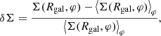
In this section, we provide details about the pattern speed measurements for individual spiral arms. In order to measure the pattern speed of the spiral arms, we analysed the stellar surface density morphology in three snapshots, one is the referenced one at t0 and the other two correspond to t0 ± 1 Myr. Thanks to the small interval between the snapshots, we could directly measure how much different radial segments of the individual spirals rotated in the azimuthal direction over 1 Myr. In practice we split each individual spiral arm into δRgal = 0.1 kpc segments and calculated the following parameter:
 (1)
(1)
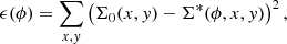
where Σ0(x, y) is the stellar surface density at t0 and Σ*(ϕ, x, y) is the stellar surface density at t0 − 1 Myr (or t0 + 1 Myr) rotated by ϕ in the azimuthal direction. Since the amplitude of the spiral arms does not change much over 1 Myr, as a result of the procedure for each segment of the spiral arms, we have a curve ϵ(ϕ) with a global minimum at the angle corresponding to the best similarity between the arm at t0 and t0 ± 1 Myr (see Fig. 1 left for a single spiral arm in M1 model). In other words, we are trying to find the angle of rotation of a given spiral arm segment over 1 Myr (backwards and forwards in time). Therefore, the angular offset corresponding to the minima of the curves in Fig. 1 left divided by 1 Myr results in the pattern speed of the spiral arm segments, or the pattern speed of individual arms as the function of Rgal (see the right panel). Since we have an opportunity to measure the rotation of spirals backwards and forwards in time, we present the curves ϵ(ϕ) for t0 − (t0 + 1 Myr) and (t0 + 1 Myr)−t0, where the minima for each Rgal are marked by circles and squares, respectively.
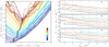 |
Fig. 1. Example of the pattern speed measurement for a single spiral arm in model M1. Left: coloured lines correspond to the sum of the squared-root differences between the stellar density at t0 = 0.6 Gyr and the ones from t0 ± 1 Myr rotated by a certain angle ϕ (see Eq. (1)). The minimum value corresponds to the angle of rotation which being divided by 1 Myr results in the pattern speed value (black symbols) at a given Rgal. Right: pattern speed of the spiral arms in different models. Values for the individual spiral arms are shown by the error bars of different colours. For a better representation, the pattern speed for each arm is shifted vertically by 10 km s−1 kpc−1 and compared to the circular frequency (solid lines) which is also shifted by the same values. |
In Fig. 1 (right) we show the pattern speed of the individual arms (crosses) compared to the rotational frequency (circular velocity divided by Rgal, solid lines) shown for each pattern speed with the same colour. For a better visibility, both the pattern speed and the corresponding rotational frequency are shifted by 10 km s−1 for different arms. As we can see, the spiral arms in our model, similar to a number of other N-body-hydrodynamical simulations (see, e.g., Wada et al. 2011; Grand et al. 2012; Roca-Fàbrega et al. 2013), do not rotate with the same pattern speed along the radius. This behaviour makes our results qualitatively similar to the ones presented in Sánchez-Menguiano et al. (2016).
3. Results
3.1. Spiral structure properties and small-scale metallicity behaviour
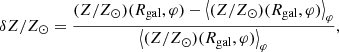
For each simulation, we focused our analysed on a single snapshot at t0 = 0.6 Gyr of evolution, when a well-formed spiral structure is present. At later times the models are unstable to bar formation which substantially impacts both stars and the ISM, analyses of which is beyond the scope of the present study. In Fig. 2 we show the face-on distributions of the stellar (first column) and gas density (second column) together with the mean ISM metallicity (third column), the residual ISM metallicity (the fourth column, after the subtraction of the radial metallicity gradient, i.e. the mean metallicity at a given Rgal shown by the solid white lines in the fifth column, and the radial metallicity profile (fifth column). In the fifth column we also provide the exponential fits of the radial metallicity profiles (solid red lines, shifted vertically). The slopes of the ISM metallicity that we measured, while being mainly inherited from the initial setup, are comparable to the ones observed in the nearby disk galaxies (Sánchez et al. 2014; Belfiore et al. 2017; Kreckel et al. 2019; Zinchenko et al. 2019, 2021; Zurita et al. 2021).
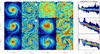 |
Fig. 2. Structure of different models after 0.6 Gyr: M1 (no initial gradient), M2 (both ISM enrichment and gradient) and M3 (only gradient). From left to right: stellar density, gas density, the mean ISM metallicity, residual ISM metallicity (after subtraction of the radial gradient), and the radial metallicity profile. Different models are shown in different rows. Coloured lines highlight the location of the stellar spiral arms measured as a positive overdensity in the first row (see Sect. 3 for details). In the right column, the mean radial metallicity trend is shown by the white solid line. The exponential fit of the radial gradient is shown by the red lines (shifted vertically for better visibility), where R25 = 12 kpc. |
Although our initial setup (mass model and initial equilibrium state) is the same in all the models, the morphology of the spiral structure is slightly different at the same snapshot in time. This is likely the result of stochasticity of the growth of the perturbations in stellar-gaseous disks (see, e.g., Romeo & Wiegert 2011) due to different ISM dynamics caused by metallicity-dependent gas cooling rates. Nevertheless, a Fourier analysis of the snapshots suggests that the modal composition of the spiral structure is very similar (see the radial structure of Fourier harmonics in Fig. 3 (top row) and all three models reveal a multi-arm, tightly wound spiral structure similar to the one usually obtained in N-body simulations. It is seen that the spiral arm structure, revealed by the Fourier analysis, is dominated by the m = 2 and m = 3 modes, for which superposition results in a slightly different morphology among our models (see Fig. 2, left) at a given time.
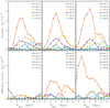 |
Fig. 3. Radial structure of the main (m = 1, …, 6) 2D Fourier harmonics computed from the stellar surface density maps (top) and from the mean metallicity distribution (bottom). |
In order to quantify the ISM metallicity behaviour in the vicinity of the spirals, we localized the individual arms which we define as the positive part of 2D stellar density perturbation (overdensity):
 (2)
(2)
where Rgal and φ are the radius and azimuth in cylindrical coordinates and the brackets ⟨⟩φ indicate the mean – that is to say azimuthally averaged value at a given Rgal. In Fig. 2 the stellar spiral arms are highlighted by coloured lines spanning the 2 kpc radial Rgal range. Although, the ISM morphology is quite complicated because of a number of chains of giant clumps near the arms and isolated clouds in between the arms (see, e.g., Dobbs et al. 2006; Renaud et al. 2013; Fujimoto et al. 2014; Khoperskov et al. 2016; Khoperskov & Vasiliev 2017), one can see that inside Rgal ≲ 10 kpc, the maxima of the large-scale gas density distribution correspond to the leading side of the stellar spiral arms, as has been expected for slowly rotating spirals (see, e.g., Dobbs & Bonnell 2006; Khoperskov et al. 2011; Pettitt et al. 2016).
In order to test the impact of the local enrichment and the radial gradient transformation on the azimuthal variations in metallicity, one needs to be sure that both the strength and pattern speed of spiral arms are the same in different models. We have shown that the amplitudes of stellar density perturbations are essentially the same in all the models (see Fig. 3, top). Also, the spiral arms for all three models rotate slower than the gas in the inner disk (≲8 − 10 kpc) and co-rotate with the gas in the outer disk (see Fig. 1, the right panel). Therefore, the material stellar arms are not steady; they are wound and, likely, stretched by the galactic shear in the outer disk. In the inner disk, spirals can bifurcate and merge with the other spirals (see, e.g., Sellwood 2011; Fujii et al. 2011). This also makes the ISM structures and abundance patterns associated with the stellar arms unsteady.
In Fig. 2 (see the third column) the mean metallicity distributions show a spiral-like morphology which, however, differs from the ones seen in gas and stars. To quantify the strength of the azimuthal metallicty variations, similar to the stellar overdensity (see Eq. (2)), we derived the residual metallicity:
 (3)
(3)
where ⟨(Z/Z⊙)(Rgal,φ)⟩φ is the azimuthally averaged radial metallicity profile (see the white lines in Fig 2, fifth column). Maps in Fig. 2 (fourth column) demonstrate that the residual metallicity varies from negative to positive values across the arms. In particular, we find that at a given Rgal, the scatter is about 0.05 dex which is similar to the numbers obtained in different observations (e.g., Zinchenko et al. 2016; Kreckel et al. 2019). To demonstrate that, in Fig. 4 we show the cumulative distribution of the absolute values of the residual metallicity for different models. The figure shows that the metallicity deviates from the mean value at a given radius by 0.05 dex for 40 − 65% of cases.
 |
Fig. 4. Cumulative distribution of the residual metallicity (after subtraction of the radial metallicity gradient) in different models. |
3.2. Large-scale metallicity behaviour across the spiral arms
In Fig. 2 we can notice that in M1, the residual metallicity does not reveal a large-scale spiral pattern, but it instead consists of a number of patchy segments. On the other hand, in models M2 and M3, the regions of systematically lower (higher) metallicity span across the entire disk. This is highlighted more quantitatively in Fig. 3, where the radial profile of Fourier coefficients is presented. In these models, one can see a dominant m = 2, 3 mode (more prominent in negative δZ, fourth column in Fig. 2), despite the presence of six spiral arms. This result suggests that the large-scale metallicity pattern, in the presence of a radial gradient, likely follows the dominant spiral mode (see Figs. 2 and 3).
In observations, the information about the ISM metallicity distribution is often based on the data from the HII regions (see, e.g., Kennicutt & Garnett 1996; Cedrés et al. 2012; Vogt et al. 2017; Kreckel et al. 2019), where the gas density is high enough to sustain recent SF. This usually does not allow for a mapping of the metallicity distribution everywhere in the disk and limits the analysis to some sparsely distributed regions. In our simulations, we were not able to resolve individual HII regions; however, to link the observational results with our models, we first limited the analysis of the ISM metallicity to the regions with high gas density. In Fig. 5 we show the distribution of the residual metallicity where we masked the regions with the gas surface density below given values (0.4, 1.4, and 5 M⊙ pc−2). Obviously, once we moved to the metallicity distribution in regions with higher gas density, the coverage of the disk decreased and the remaining regions traced the spiral arms better. However, there is no prominent systematics in the residual metallicity values in the remaining high-gas density regions. In particular, the second and third columns of Fig. 5 show that the residual metallicity varies in a wide range where the entire arms or their small patches can systematically have either positive or negative values for the residual metallicity. If, following some theoretical expectations (Sánchez-Menguiano et al. 2016; Ho et al. 2017; Spitoni et al. 2019), the high-metallicity ISM is associated with the spiral arms then the mean of the metallicity distribution should move towards positive values once low-gas density regions are masked. To test this, we show the distribution of the residual metallicity in the regions with high gas density in the rightmost column in Fig. 5. In other words, we plotted the distribution of the values from maps shown in the first three columns of Fig. 5. The resulting distributions, however, do not vary significantly, and both the mean and its dispersion are weakly impacted by the spatial selections based on the gas surface density. This suggests that similar to a number of observational studies, there is no apparent match between the large-scale metallicity patterns and the spiral arms in our models. However, since Fig. 2 shows the metallicity distributions still demonstrating certain patterns, in the following, we analyse the complete metallicity distributions without masking any low gas-density regions.
 |
Fig. 5. Residual ISM metallicity maps. The regions with different minimal gas surface density are shown, from left to right: Σgas > 0.4 M⊙ pc−2, Σgas > 1.4 M⊙ pc−2 and Σgas > 5 M⊙ pc−2. The rightmost column shows the distribution of the residual metallicity in the corresponding disk regions. Once the regions with lower gas density are masked, the remaining areas follow the stellar spiral arms much closer; however, the residual metallicity distributions are weakly affected by these selections. The pairs of numbers in the rightmost column show the mean and the standard deviation of the residual metallicity distributions. |
To analyze the variations in the metallicity more quantitatively, we show the residual metallicity distributions for all spiral arms and inter-arm region (top) and for individual spiral arms (bottom) in Fig. 6. We see that the residual metallicities for both arm and inter-arms regions vary in roughly the same range, while spiral arm regions have slightly higher metallicities. The effect is the most prominent in model M3 (without enrichment), suggesting that the release of metals by newly formed stars does not correlate with the spiral arms much, but it tends to smear the metallicity distribution at a given Rgal (see, e.g., Yang & Krumholz 2012; Krumholz & Ting 2018).
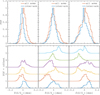 |
Fig. 6. Probability distribution functions for the residual ISM metallicity in arms and inter-arm regions (top). The bottom row shows the corresponding PDFs for individual spiral arms where the colour of the lines is the same as in Fig. 2. |
The distributions in Fig. 6 suggest that systematically negative residuals in metallicity do occur in some of the spiral arms. This contradicts naive expectations that SF would locally increase the ISM metallicity. To search for the latter effect, we found the location of nearby positive peaks in metallicity next to the arms and, thus, measured the offset to the spiral arms. In Fig. 7 (top), we show two examples of the offset calculation for the pair of arms in M1 and M3 models. One can see that there is a positive (larger Rgal) offset of the metallicity peak (dashed lines) to the blue arm (solid) in M1, while in model M3 we see the opposite configuration (the peak of metallicity has systematically smaller Rgal relative to the stellar spiral arm). For the red arms in both models, the offset is, on average, zero. Of course, the offset we calculated may not represent a generic connection between the spiral arms and metallicity distribution, especially at small spatial scales; however, it gives an idea of how, on average, the spatial distribution of metals correlates with the spiral arms depending on the initial radial gradient and ISM enrichment. In the bottom panel of Fig. 7, we show the distribution of the offset for all the arms in the three models. The models with an initial radial gradient (M2 and M3) show, on average, a negative radial offset between the spiral arm and metallicity peak, suggesting the presence of higher metallicity behind the trailing arms. In M1, the offset distribution is roughly symmetric. This behaviour is likely linked to the SF activity where newborn stars can release metals far away from their birthplaces in the spirals or even reach other arms, especially in the inner disk, where spirals rotate slower than the gas, thus breaking a coherent cycle of enrichment and mixing proposed in some previous works (Ho et al. 2017; Spitoni et al. 2019).
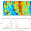 |
Fig. 7. Offset between spiral arms and the ISM metallicity. Top: background maps are the residual ISM metallicity in model M1 (no radial gradient, left) and M3 (no ISM enrichment, right) where the location of the stellar spiral arms is shown with solid lines, while the mean location of the metallicity peaks is shown with dashed lines. Bottom: distribution of the radial offset between the mean location of the stellar spiral arms and the metallicity peaks for different models. |
To test the hypothesis about the impact of local enrichment further, in Fig. 8, we show the relation between the SF surface density and the metallicity residuals. The relation is based on the 500 × 500 pc2 smoothing of both SFR and δZ metallicity XY maps. Although we do not see a strong correlation for any of our models, in M1, there is a clear trend where more metal-rich regions tend to be spatially associated with more intense SF. Finally, we tested how much the ISM dynamics affects the appearance of the large-scale abundance variations in the azimuthal direction.
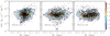 |
Fig. 8. Relations between the residual metallicity and SF surface density. Coloured lines represent the density contours. The corresponding Pearson correlation coefficients are given in each panel. |
In Fig. 9 we compare the relation between both radial (VR) and residual azimuthal velocity (δVφ) components of the gas with the residual metallicity. The residual azimuthal velocity component is the gas velocity component after the subtraction of the mean azimuthally averaged rotation (rotation curve, see Eq. (2) where Σ should be replaced by Vφ). We see no correlation in the case of M1 (only enrichment) and a very clear correlation for M3 (no enrichment, but an initial radial gradient), while model M2 shows an intermediate behaviour. Similar to the SFR − δZ analysis in Fig. 8, we calculated the Pearson correlation coefficients which allowed us to quantify the relations between the gas velocity components and the residual ISM metallicity (see numbers in the panels of Fig. 9). This result suggests that, even slowly (compared to gas), rotating spiral arms drag a more metal-rich gas from the inner parts of the disk to the trailing side of the arms, thus increasing the mean metallicity of the ISM behind the spirals. This picture explains why in models M2 and M3 we find a prominent negative offset of the metallicity peaks relative to the spiral arms (see Fig. 7).
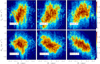 |
Fig. 9. Relations between the residual metallicity and gas radial velocity component (top) and residual azimuthal velocity component (subtracted circular velocity, bottom). The colours represent the mass fraction of the gas. |
4. Summary
Using hydrodynamical simulations of isolated spiral galaxies, we study the impact of the local enrichment and pre-existing radial metallicity gradient transformation on the formation of azimuthal metallicity variations in the vicinity of the spiral arms. Similar to some previous studies, in our models, the pattern speed of individual arms varies with the radius being slow (compared to the disk rotation) in the inner disk (< 8 kpc) and co-rotating in the outer disk. Our main results are as follows.
-
Both types of models with local enrichment and a pre-existing radial abundance gradient are able to produce the azimuthal scatter of the ISM metallicity (≈0.05 dex) in simulated spiral galaxies (see Fig. 2). Analysis of the ISM metallicity as a function of the underlying gas density does not reveal any strong relations between the residual metallicity and the location of the stellar spiral arms (see Fig. 5). Although individual arms could have systematically lower or higher (than the mean) metallicity, gas in the spiral is slightly more metal-rich compared to the inter-arms region (see Fig. 6).
-
We find that the model with local enrichment only (M1, no pre-existing metallicity gradient) is not able to reproduce large-scale spiral-arm-like variations in the mean metallicity (see Figs. 2 and 3). In this model, the short-scale patches of high-metallicity regions can be found suggesting that the enrichment of the ISM does not correlate with the large-scale spiral structure much.
-
Both models with a pre-existing radial metallicity gradient (M2 and M3) show the formation of a spiral-like metallicity pattern, but its morphology differs from the stellar spiral structure (see Fig. 2). Although we identified a six-armed spiral structure, the large-scale residual metallicity pattern depicts an m = 2, 3 structure, corresponding to the most significant 2D Fourier harmonics of the stellar density distribution (see Fig. 3).
-
We found a substantial radial offset between spiral arms and the metal-rich ISM pattern. The amplitude of the offset reaches up to 1 − 1.5 kpc (see Fig. 7). In models with a radial gradient, we found no correlation between the residual metallicity with recent SF. On the other hand, in model M1, without a gradient, we can see a weak increase in the metallicity with higher SF. The model without ISM enrichment shows the most prominent correlation of the residual metallicity with the gas velocity components: larger metallicity corresponds to larger negative (inflow) radial velocities and negative azimuthal velocity residuals. Therefore, we suggest that dynamical effects play a key role in the formation of the large-scale metallicity variations across spiral arms.
Our models, while being rather simplified, nevertheless allow us to propose an explanation for the observational data demonstrating a controversial picture in the systematic azimuthal variations of metallicity around spiral arms. We suggest that the ISM enrichment near the arms alone is not likely responsible for the systematic azimuthal metallicity pattern, at least in the case of non-steady spirals, while the key ingredient is a pre-existing radial abundance gradient. If the observed radial gradients are small (Sánchez et al. 2014), they are likely not enough to be transformed into the azimuthal variations in most of the galaxies. However, once the azimuthal variations are found, they will more likely depict the shape of the most significant spiral mode (m = 2, 3), which can explain prominent oxygen variations found in some barred galaxies (Sánchez-Menguiano et al. 2016; Ho et al. 2017). Nevertheless, in some cases, flattening of the radial gradient should act against the formation of the systematic azimuthal variations.
Extending the model presented in Sánchez-Menguiano et al. (2016), we suggest that co-rotating spirals responsible for azimuthal variations in ISM metallicity, but also slowly (compared to the gas) rotating patterns provide similar results. Obviously, our predictions will depend on the strength and nature of the spirals and also SF activity, which, along with the Fourier analysis of the 2D metallicity distribution, may be tested by IFU surveys in the near future.
We note that Grand et al. (2016) and Di Matteo et al. (2013) discuss the abundance variations in stellar populations but not in the ISM.
Acknowledgments
SK deeply appreciates Igor Zinchenko (LMU, Munich; MAO, Kyiv) for his contribution to the early versions of the paper. The authors thank the anonymous referee for a constructive report. SK also thanks Daisuke Kawata for useful discussion about the nature of co-rotating spirals. Numerical simulations were carried by using the equipment of the shared research facilities of HPC computing resources at Lomonosov Moscow State University (project RFMEFI62117X0011) supported by the Russian Science Foundation (project no. 19-72-20089).
References
- Belfiore, F., Maiolino, R., Tremonti, C., et al. 2017, MNRAS, 469, 151 [Google Scholar]
- Bird, J. C., Kazantzidis, S., Weinberg, D. H., et al. 2013, ApJ, 773, 43 [Google Scholar]
- Brook, C. B., Stinson, G. S., Gibson, B. K., et al. 2012, MNRAS, 426, 690 [Google Scholar]
- Cedrés, B., Cepa, J., Bongiovanni, Á., et al. 2012, A&A, 545, A43 [NASA ADS] [CrossRef] [EDP Sciences] [Google Scholar]
- Chiappini, C., Matteucci, F., & Gratton, R. 1997, ApJ, 477, 765 [Google Scholar]
- Croxall, K. V., Pogge, R. W., Berg, D. A., Skillman, E. D., & Moustakas, J. 2016, ApJ, 830, 4 [NASA ADS] [CrossRef] [Google Scholar]
- de Avillez, M. A., & Mac Low, M.-M. 2002, ApJ, 581, 1047 [NASA ADS] [CrossRef] [Google Scholar]
- Di Matteo, P., Haywood, M., Combes, F., Semelin, B., & Snaith, O. N. 2013, A&A, 553, A102 [NASA ADS] [CrossRef] [EDP Sciences] [Google Scholar]
- Dobbs, C. L., & Bonnell, I. A. 2006, MNRAS, 367, 873 [NASA ADS] [CrossRef] [Google Scholar]
- Dobbs, C. L., Bonnell, I. A., & Pringle, J. E. 2006, MNRAS, 371, 1663 [Google Scholar]
- Fujii, M. S., Baba, J., Saitoh, T. R., et al. 2011, ApJ, 730, 109 [NASA ADS] [CrossRef] [Google Scholar]
- Fujimoto, Y., Tasker, E. J., Wakayama, M., & Habe, A. 2014, MNRAS, 439, 936 [NASA ADS] [CrossRef] [Google Scholar]
- Fukushige, T., Makino, J., & Kawai, A. 2005, PASJ, 57, 1009 [NASA ADS] [CrossRef] [Google Scholar]
- Gibson, B. K., Pilkington, K., Brook, C. B., Stinson, G. S., & Bailin, J. 2013, A&A, 554, A47 [CrossRef] [EDP Sciences] [Google Scholar]
- Grand, R. J. J., Kawata, D., & Cropper, M. 2012, MNRAS, 426, 167 [NASA ADS] [CrossRef] [Google Scholar]
- Grand, R. J. J., Springel, V., Kawata, D., et al. 2016, MNRAS, 460, L94 [Google Scholar]
- Grand, R. J. J., Bustamante, S., Gómez, F. A., et al. 2018, MNRAS, 474, 3629 [NASA ADS] [CrossRef] [Google Scholar]
- Ho, I. T., Seibert, M., Meidt, S. E., et al. 2017, ApJ, 846, 39 [NASA ADS] [CrossRef] [Google Scholar]
- Kennicutt, R. C., Jr, & Garnett, D. R. 1996, ApJ, 456, 504 [NASA ADS] [CrossRef] [Google Scholar]
- Khoperskov, S. A., & Vasiliev, E. O. 2017, MNRAS, 468, 920 [CrossRef] [Google Scholar]
- Khoperskov, S. A., Khoperskov, A. V., Eremin, M. A., & Butenko, M. A. 2011, Astron. Lett., 37, 563 [NASA ADS] [CrossRef] [Google Scholar]
- Khoperskov, S. A., Vasiliev, E. O., Khoperskov, A. V., & Lubimov, V. N. 2014, J. Phys. Conf. Ser., 510, 012011 [CrossRef] [Google Scholar]
- Khoperskov, S. A., Vasiliev, E. O., Ladeyschikov, D. A., Sobolev, A. M., & Khoperskov, A. V. 2016, MNRAS, 455, 1782 [NASA ADS] [CrossRef] [Google Scholar]
- Khoperskov, S., Di Matteo, P., Haywood, M., & Combes, F. 2018, A&A, 611, L2 [NASA ADS] [CrossRef] [EDP Sciences] [Google Scholar]
- Khoperskov, S., Di Matteo, P., Haywood, M., Gómez, A., & Snaith, O. N. 2020, A&A, 638, A144 [NASA ADS] [CrossRef] [EDP Sciences] [Google Scholar]
- Khoperskov, S., Haywood, M., Snaith, O., et al. 2021, MNRAS, 501, 5176 [NASA ADS] [CrossRef] [Google Scholar]
- Klessen, R. S., & Lin, D. N. 2003, Phys. Rev. E, 67, 046311 [NASA ADS] [CrossRef] [Google Scholar]
- Kreckel, K., Blanc, G. A., Schinnerer, E., et al. 2016, ApJ, 827, 103 [NASA ADS] [CrossRef] [Google Scholar]
- Kreckel, K., Ho, I. T., Blanc, G. A., et al. 2019, ApJ, 887, 80 [NASA ADS] [CrossRef] [Google Scholar]
- Krumholz, M. R., & Ting, Y.-S. 2018, MNRAS, 475, 2236 [NASA ADS] [CrossRef] [Google Scholar]
- Li, Y., Bresolin, F., & Kennicutt, R. C., Jr 2013, ApJ, 766, 17 [NASA ADS] [CrossRef] [Google Scholar]
- Matteucci, F., & Francois, P. 1989, MNRAS, 239, 885 [Google Scholar]
- Minchev, I., & Famaey, B. 2010, ApJ, 722, 112 [Google Scholar]
- Minchev, I., Famaey, B., Combes, F., et al. 2011, A&A, 527, A147 [NASA ADS] [CrossRef] [EDP Sciences] [Google Scholar]
- Minchev, I., Chiappini, C., & Martig, M. 2013, A&A, 558, A9 [CrossRef] [EDP Sciences] [Google Scholar]
- Minchev, I., Chiappini, C., & Martig, M. 2014, A&A, 572, A92 [CrossRef] [EDP Sciences] [Google Scholar]
- Minchev, I., Anders, F., Recio-Blanco, A., et al. 2018, MNRAS, 481, 1645 [NASA ADS] [CrossRef] [Google Scholar]
- Miyamoto, M., & Nagai, R. 1975, PASJ, 27, 533 [NASA ADS] [Google Scholar]
- Pettitt, A. R., Tasker, E. J., & Wadsley, J. W. 2016, MNRAS, 458, 3990 [CrossRef] [Google Scholar]
- Pilkington, K., Few, C. G., Gibson, B. K., et al. 2012, A&A, 540, A56 [NASA ADS] [CrossRef] [EDP Sciences] [Google Scholar]
- Plummer, H. C. 1911, MNRAS, 71, 460 [Google Scholar]
- Quillen, A. C., Minchev, I., Bland-Hawthorn, J., & Haywood, M. 2009, MNRAS, 397, 1599 [NASA ADS] [CrossRef] [Google Scholar]
- Renaud, F., Bournaud, F., Emsellem, E., et al. 2013, MNRAS, 436, 1836 [NASA ADS] [CrossRef] [Google Scholar]
- Roca-Fàbrega, S., Valenzuela, O., Figueras, F., et al. 2013, MNRAS, 432, 2878 [Google Scholar]
- Romeo, A. B., & Wiegert, J. 2011, MNRAS, 416, 1191 [NASA ADS] [CrossRef] [Google Scholar]
- Roškar, R., Debattista, V. P., Quinn, T. R., Stinson, G. S., & Wadsley, J. 2008, ApJ, 684, L79 [Google Scholar]
- Saburova, A. S., Chilingarian, I. V., Katkov, I. Y., et al. 2018, MNRAS, 481, 3534 [CrossRef] [Google Scholar]
- Sakhibov, F., Zinchenko, I. A., Pilyugin, L. S., et al. 2018, MNRAS, 474, 1657 [CrossRef] [Google Scholar]
- Sánchez, S. F., Rosales-Ortega, F. F., Iglesias-Páramo, J., et al. 2014, A&A, 563, A49 [CrossRef] [EDP Sciences] [Google Scholar]
- Sánchez-Blázquez, P., Courty, S., Gibson, B. K., & Brook, C. B. 2009, MNRAS, 398, 591 [CrossRef] [Google Scholar]
- Sánchez-Menguiano, L., Sánchez, S. F., Kawata, D., et al. 2016, ApJ, 830, L40 [CrossRef] [Google Scholar]
- Sánchez-Menguiano, L., Sánchez, S. F., Pérez, I., et al. 2020, MNRAS, 492, 4149 [CrossRef] [Google Scholar]
- Sellwood, J. A. 2011, MNRAS, 410, 1637 [NASA ADS] [Google Scholar]
- Sellwood, J. A., & Binney, J. J. 2002, MNRAS, 336, 785 [Google Scholar]
- Spitoni, E., Cescutti, G., Minchev, I., et al. 2019, A&A, 628, A38 [NASA ADS] [CrossRef] [EDP Sciences] [Google Scholar]
- Vasiliev, E. 2019, MNRAS, 482, 1525 [Google Scholar]
- Vogt, F. P. A., Pérez, E., Dopita, M. A., Verdes-Montenegro, L., & Borthakur, S. 2017, A&A, 601, A61 [NASA ADS] [CrossRef] [EDP Sciences] [Google Scholar]
- Wada, K., Baba, J., & Saitoh, T. R. 2011, ApJ, 735, 1 [NASA ADS] [CrossRef] [Google Scholar]
- Williams, T. G., Kreckel, K., Belfiore, F., et al. 2021, MNRAS, 509, 1303 [NASA ADS] [CrossRef] [Google Scholar]
- Yang, C.-C., & Krumholz, M. 2012, ApJ, 758, 48 [NASA ADS] [CrossRef] [Google Scholar]
- Zinchenko, I. A., Pilyugin, L. S., Grebel, E. K., Sánchez, S. F., & Vílchez, J. M. 2016, MNRAS, 462, 2715 [Google Scholar]
- Zinchenko, I. A., Just, A., Pilyugin, L. S., & Lara-Lopez, M. A. 2019, A&A, 623, A7 [NASA ADS] [CrossRef] [EDP Sciences] [Google Scholar]
- Zinchenko, I. A., Vilchez, J. M., Perez-Montero, E., et al. 2021, A&A, 655, A58 [NASA ADS] [CrossRef] [EDP Sciences] [Google Scholar]
- Zurita, A., Florido, E., Bresolin, F., Pérez, I., & Pérez-Montero, E. 2021, MNRAS, 500, 2380 [Google Scholar]
All Figures
|
Fig. 1. Example of the pattern speed measurement for a single spiral arm in model M1. Left: coloured lines correspond to the sum of the squared-root differences between the stellar density at t0 = 0.6 Gyr and the ones from t0 ± 1 Myr rotated by a certain angle ϕ (see Eq. (1)). The minimum value corresponds to the angle of rotation which being divided by 1 Myr results in the pattern speed value (black symbols) at a given Rgal. Right: pattern speed of the spiral arms in different models. Values for the individual spiral arms are shown by the error bars of different colours. For a better representation, the pattern speed for each arm is shifted vertically by 10 km s−1 kpc−1 and compared to the circular frequency (solid lines) which is also shifted by the same values. |
| In the text | |
|
Fig. 2. Structure of different models after 0.6 Gyr: M1 (no initial gradient), M2 (both ISM enrichment and gradient) and M3 (only gradient). From left to right: stellar density, gas density, the mean ISM metallicity, residual ISM metallicity (after subtraction of the radial gradient), and the radial metallicity profile. Different models are shown in different rows. Coloured lines highlight the location of the stellar spiral arms measured as a positive overdensity in the first row (see Sect. 3 for details). In the right column, the mean radial metallicity trend is shown by the white solid line. The exponential fit of the radial gradient is shown by the red lines (shifted vertically for better visibility), where R25 = 12 kpc. |
| In the text | |
|
Fig. 3. Radial structure of the main (m = 1, …, 6) 2D Fourier harmonics computed from the stellar surface density maps (top) and from the mean metallicity distribution (bottom). |
| In the text | |
|
Fig. 4. Cumulative distribution of the residual metallicity (after subtraction of the radial metallicity gradient) in different models. |
| In the text | |
|
Fig. 5. Residual ISM metallicity maps. The regions with different minimal gas surface density are shown, from left to right: Σgas > 0.4 M⊙ pc−2, Σgas > 1.4 M⊙ pc−2 and Σgas > 5 M⊙ pc−2. The rightmost column shows the distribution of the residual metallicity in the corresponding disk regions. Once the regions with lower gas density are masked, the remaining areas follow the stellar spiral arms much closer; however, the residual metallicity distributions are weakly affected by these selections. The pairs of numbers in the rightmost column show the mean and the standard deviation of the residual metallicity distributions. |
| In the text | |
|
Fig. 6. Probability distribution functions for the residual ISM metallicity in arms and inter-arm regions (top). The bottom row shows the corresponding PDFs for individual spiral arms where the colour of the lines is the same as in Fig. 2. |
| In the text | |
|
Fig. 7. Offset between spiral arms and the ISM metallicity. Top: background maps are the residual ISM metallicity in model M1 (no radial gradient, left) and M3 (no ISM enrichment, right) where the location of the stellar spiral arms is shown with solid lines, while the mean location of the metallicity peaks is shown with dashed lines. Bottom: distribution of the radial offset between the mean location of the stellar spiral arms and the metallicity peaks for different models. |
| In the text | |
|
Fig. 8. Relations between the residual metallicity and SF surface density. Coloured lines represent the density contours. The corresponding Pearson correlation coefficients are given in each panel. |
| In the text | |
|
Fig. 9. Relations between the residual metallicity and gas radial velocity component (top) and residual azimuthal velocity component (subtracted circular velocity, bottom). The colours represent the mass fraction of the gas. |
| In the text | |
Current usage metrics show cumulative count of Article Views (full-text article views including HTML views, PDF and ePub downloads, according to the available data) and Abstracts Views on Vision4Press platform.
Data correspond to usage on the plateform after 2015. The current usage metrics is available 48-96 hours after online publication and is updated daily on week days.
Initial download of the metrics may take a while.