| Issue |
A&A
Volume 670, February 2023
|
|
|---|---|---|
| Article Number | A143 | |
| Number of page(s) | 7 | |
| Section | Stellar structure and evolution | |
| DOI | https://doi.org/10.1051/0004-6361/202245309 | |
| Published online | 16 February 2023 | |
How noise thresholds affect the information content of stellar flare sequences
1
Andrews University, 8975 Old 31, Berrien Springs, MI 49103, USA
e-mail: This email address is being protected from spambots. You need JavaScript enabled to view it.
2
Johns Hopkins University, Applied Physics Laboratory, 11100 Johns Hopkins Rd, Laurel, MD 20723, USA
Received:
27
October
2022
Accepted:
30
November
2022
Abstract
Systems that exhibit discrete dynamics can be well described and reconstructed by considering the set of time intervals between the discrete events of the system. The Kepler satellite has cataloged light curves for many Sun-like stars, and these light curves show strong bursts in intensity that are associated with stellar flares. The waiting time between these flares describes the fundamental dynamics of the stars and is driven by physical processes, such as flux emergence. While it is rather straightforward to identify large flares, the identification of weaker flares can be challenging because of the presence of noise. A common practice is to limit flare identification to events stronger than a threshold value that significantly exceeds the noise level (kσ), where σ is the standard deviation of the fluctuations about the detrended light curve. However, the selection of the k-value is normally made based on an empirical rule (typically k = 3), which can lead to a biased threshold level. This study examines the information content in the waiting time sequence of enhancements in the light curve of a solar-type star (KIC 7985370) as a function of threshold. Information content is quantified by the mutual information between successive flare waiting times. It is found that the information content increases as the threshold is reduced from k = 3 to k = 1.56, in contrast with the notion that low amplitude enhancements are simply random noise. However, below k = 1.56 the information content dramatically decreases, consistent with shot noise. The information that is detected at k = 1.56 and above is similar to that of solar flares and indicates a significant relationship between the low amplitude enhancements, suggesting that many of those events are likely flares. We suggest that mutual information could be used to identify a threshold that maximizes the information content of the flare sequence, making it possible to extract more flare information from stellar light curves.
Key words: stars: flare / stars: solar-type / methods: statistical
© E. C. Rivera et al. 2023
 Open Access article, published by EDP Sciences, under the terms of the Creative Commons Attribution License (https://creativecommons.org/licenses/by/4.0), which permits unrestricted use, distribution, and reproduction in any medium, provided the original work is properly cited.
This article is published in open access under the Subscribe-to-Open model. This email address is being protected from spambots. You need JavaScript enabled to view it. to support open access publication.
1. Introduction
The Kepler mission (Borucki et al. 2010) has opened a new era in the study of flares (Yang & Liu 2019). The flare catalog (Davenport 2016; Yang & Liu 2019) now includes at least 3400 flare stars with over 160 000 flare events. These flares provide an excellent context for understanding flare dynamics at the Sun and how it may be evolving. Considering that stellar flares most likely result from the same mechanism as solar flares, the study of solar-type stars makes it possible to understand whether the Sun can really serve as a reliable calibrator of stellar evolution, or whether it instead is an outlier among stars of its age and mass (Fabbian et al. 2017). Typical flare profiles and the occurrence frequency are similar to those the Sun (Maehara et al. 2012; Shibayama et al. 2013; Yang et al. 2017). However, there can be substantial differences in terms of their typical energy, mean flaring rate, and spectra.
A key task in studying stellar flares is the identification of flares in the Kepler light curves. The catalogs that have been compiled typically use a specific set of criteria (Davenport 2016; Yang & Liu 2019). Flares are generally identified as impulsive, sustained, large amplitude excursions in the Kepler light curve relative to background fluctuations. The process of flare identification typically involves detrending and filtering the data and then identifying candidate flares whose amplitude exceeds a threshold based on the background noise level. Candidate events below this threshold are discarded as indistinguishable from noise. To be entered into the catalog, the flares must also pass additional selection criteria to remove artifacts such as pulsating stars (Aerts et al. 2010; Balona et al. 2011) or instrumental error (Yang et al. 2018).
In the procedure for the selection of flare candidates, the threshold condition is somewhat arbitrary, but a 3σ rule is most commonly applied (Mossoux & Grosso 2017; Oláh et al. 2021). Nevertheless, the use of 2σ has also been reported (Stelzer et al. 2020). Other studies of solar flares have required the peak flux of a flare to exceed an arbitrary threshold value, for example class C1 and above (Wheatland & Litvinenko 2002; Snelling et al. 2020), to reflect the difficulty of detecting flares below class C1. Methods based on machine learning models have been tested as well (Vida & Roettenbacher 2018; Feinstein et al. 2020) to better automate flare detection; however, their performance is highly dependent on the quality of data available for training the models.
In this paper we explore how the choice of threshold can affect flare identification using information theory, and in particular we show that many significant events discarded as noise based on an arbitrary threshold have characteristics that are very different from noise. It is possible that these events are actually real flares of relatively low amplitude, as typically found at the Sun (Hannah et al. 2011).
2. Data – KIC 7985370
For this study we considered the solar-type star KIC 7985370, an active early-G-type main-sequence star that has previously been studied in detail (Fröhlich et al. 2012). This star is reported to be a young star, with an age of about 100–200 Myr, that has a faster rotation period (2.84–3.09 days; Fröhlich et al. 2012; Reinhold et al. 2013) than the Sun and a high level of chromospheric activity. The activity level, spot distribution, and differential rotation have been studied in detail.
The short cadence (1 min resolution) light curve of KIC 7985370 was extracted using the LightKurve1 package for the period 2009 May (Quarter 1) to 2010 August (Quarter 6). While long cadence data are available over a longer time period, the 30 min resolution of the long cadence data is not adequate for resolving flare events.
Figure 1 shows a ten-day segment of the light curve for KIC 7985370. The light curve exhibits a prominent quasi-periodic three-day rotational modulation due to the transit of persistent stellar magnetic features (i.e., dark spots and bright faculae) over the visible stellar hemisphere (Berdyugina 2005; Strassmeier 2009). Longer segments of the same light curve (see Fig. 8 of Fröhlich et al. 2012) show the same three-day rotational modulation as well as longer modulations associated with the time variability of starspots due to differential rotation and the magnetic activity cycle.
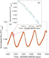 |
Fig. 1. Light curve for KIC 7985370. (a) Application of our flare selection criteria applied to the data with k = 1.56; flare events are shown as open orange circles. (b) Zoomed-in view of the group of flares in the red shaded box. |
To compensate for these underlying trends and periodicities, we followed a similar procedure as Li et al. (2018) to impose a threshold as follows: (a) the data were first separated into segments without any significant data gaps, (b) each segment was detrended and passed through a smoothing filter (moving median) with a 1 hour window, (c) the residual (high pass filtered) time series was then obtained by subtracting the detrended data from the stellar intensity data. Flares were identified in the residual time series using the MATLAB2 findpeaks function with the requirement that flares have a minimum separation of 10 min and the peak prominence is kσ, where σ is the standard deviation and k is a positive real number.
Because strong flare events skew the distribution of the residuals, we excluded outlier events when computing σ by (a) first computing the standard deviation of the detrended light curve, (b) excluding all events exceeding 3σ, and (c) recomputing the standard deviation after the outlier data were excluded. Following this procedure, we constructed data sets with values of k less than 3. The number of flares identified increased from 654 at k = 3 to 7213 at k = 1.56 and 16 724 at k = 0.5, consistent with an expected increase in the number of flares identified as the threshold is reduced.
In Fig. 1 flare events identified by the flare selection criteria with a threshold of k = 1.56 are shown. It is apparent that there are some groups of flares that occur in close proximity. A zoomed-in view of the group of flares shows how the clusters of flares are resolved on a shorter timescale. It should be noted that all peaks must be separated by at least 10 min so that the last light curve elevation is not considered a separate event. Several of the events in this box are well below the 3σ criterion. As the threshold increases, it is obvious that fewer candidate flares would be identified.
Because the time between flares is generally much greater than the duration of flares, it is a common practice to consider a sequence of discrete flare events occurring at times (t1, t2, …, tn, …, tNflare), which are equivalently described by the waiting time between events (Δ1, Δ2, …, Δn, …, ΔN), where Δn = tn + 1 − tn. The underlying system dynamics is then captured in this sequence of waiting times and is reflected in the hierarchy of the probability distributions p(Δn), p(Δn, Δn + m), p(Δn, Δn + m, Δn + q), ... In this notation, p(Δn) is the probability distribution of waiting times, p(Δn, Δn + m) describes the joint probability between the waiting time of a flare with that of another flare m steps ahead in the sequence, and so forth.
Many studies have recognized that the distribution of waiting times may result from specific types of processes. For example, waiting times resulting from a single parameter Poisson process fall off exponentially. When there is a Poisson process with discrete changes in the rate, the distribution may lead to a power law in the tail of the distribution and is often referred to as a nonstationary Poisson process (Wheatland & Litvinenko 2002; Aschwanden & McTiernan 2010; Nurhan et al. 2021). When the probability of an event not occurring is proportional to a power of time, the distribution takes the form of a Weibull distribution, which is a particular type of nonstationary Poisson process.
The waiting time distribution with k = 1.56 for KIC 7985370 is shown in Fig. 2. Waiting times greater than 5 hours are not shown. Waiting times longer than 5 h represent less than 0.35% of the data. Long waiting times could be indicators of erroneous data, resulting in missed events or gaps in the data due to the possible maintenance of the instrument (Snelling et al. 2020), so we did not include these data in our analysis. It is apparent that the distribution of waiting times is well fit by an exponential distribution consistent with a Poisson process. As the selection criteria (k-threshold) changes, the distribution of waiting times remains similarly exponential, although the slope changes to reflect an increase in the event rate as k decreases.
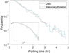 |
Fig. 2. Waiting time distribution for the entire period and stationary Poisson distribution (p ∝ 0.2423e−1.373Δ). |
It is usually thought that a waiting time distribution consistent with a Poisson distribution indicates that the events occurred independently and that the slope provides the average rate of occurrence. However, the sequence of waiting times can contain more information about the dynamics of the system than just the waiting time distribution. The joint probability distribution can tell us more specifically whether the subsequent flares are related to each other (Rivera et al. 2022). Analysis of the sequence of solar flares has shown that the flare sequence is significantly distinguishable from a nonstationary Poisson process and exhibits a short-term memory (Snelling et al. 2020; Aschwanden & Johnson 2021). This memory is associated with a clustering of flares (Rivera et al. 2022). In the next section we show that a similar memory can be identified in the stellar flare sequence of KIC 7985370.
3. Mutual information about the waiting time sequence of KIC 7985370
Information theory (Deco & Schhurmann 2000; Johnson & Wing 2018; Wing & Johnson 2019) has been widely used to identify dependence in nonlinear systems in space plasmas (Johnson & Wing 2005, 2014; Johnson et al. 2018; Wing et al. 2005, 2016, 2018, 2020, 2022; Rivera et al. 2022). Mutual information, ℳ, can be used as a metric that provides a measure of whether subsequent flares are dependent or independent, and to determine how far ahead this dependence lasts, effectively determining an information horizon for the memory of flares (Snelling et al. 2020). To determine whether there is memory in the sequence, the joint probability, p(Δn, Δn + m), between the waiting time of a flare event and another flare event with a “look ahead” of m is examined.
When m = 1, this metric measures the relationship between successive flares. The comparison described by Eq. (1) establishes whether subsequent waiting times are independent:
 (1)
(1)
The comparison is established using the mutual information, defined as
 (2)
(2)
where
 (3)
(3)
are the Shannon entropy of the random variables x ∈ X and y ∈ Y, and
 (4)
(4)
is the joint entropy. Mutual information is particularly useful for establishing nonlinear relationships between two random variables. It is evident that when X and Y are independent, ℳ(X, Y)→0, which should be the case when the flares result from a Poisson process.
As described in Snelling et al. (2020), mutual information was computed based on histogramming the data to obtain the joint and marginal waiting time distributions. We used methods similar to those outlined in Snelling et al. (2020) to optimize the bin size.
As mentioned above, the aim is to determine whether flare events are statistically independent. A Poisson process should have ℳ = 0. However, when there is a limited amount of data, ℳ can be small but nonzero. In order to interpret mutual information results from the data, we constructed an ensemble of surrogate data sets to calculate the significance (Snelling et al. 2020),
 (5)
(5)
where ℳd is the mutual information of the data, ⟨ℳsurr⟩ is the ensemble averaged mutual information obtained by averaging the mutual information of the jth surrogate data set, ℳsurr(j), over the number, Nsurr, of surrogates,
 (6)
(6)
and σsurr is the standard deviation of those surrogate mutual information calculations:
 (7)
(7)
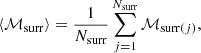
First we analyzed the waiting time sequence for flare events in the KIC 7985370 light curve when a k = 2 threshold is used. The mutual information for this case is shown in Fig. 3 (panel a) as a function of look ahead, m. For comparison, the mean and 3σ level of the surrogates is also shown. The significance as defined in Eq. (5) is shown in Fig. 3 (panel b). In this case, the surrogates are constructed with a random permutation of the waiting times, which retains the original distribution of waiting times but ensures that they are randomly drawn. Differences between the actual data and the surrogates indicate that, in this case, flares up to look ahead m = 2 are not randomly distributed and that some successive flares are related to each other. This behavior is similar to the short-term memory identified in the sequence of solar waiting times (Snelling et al. 2020). It should be noted that in the study of Snelling et al. (2020), Bayesian block analysis was used to construct the surrogates, and such a procedure was necessary to account for variability in the flare rate during the solar cycle. In this case the simpler null hypothesis that the waiting times are randomly ordered is sufficient to demonstrate the short-term memory because the distribution of waiting times is well fit by a stationary Poisson distribution (see Fig. 2).
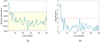 |
Fig. 3. Information content as a function of look ahead, m. (a) Mutual information with k-threshold equal to 2. Mutual information of 50 surrogates is shown as a green line, and the envelope of the 3σ the fluctuation of the surrogates is shaded yellow. Note that the look ahead axis begins at m = 1. (b) Significance of the mutual information as a function of look ahead. The significance is elevated for m = 1 and 2, indicating that successive flares have a relationship. |
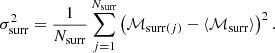
This same analysis was then applied to the flare sequences obtained by varying the k-threshold. In Fig. 4 (panel a) we show the significance as a function of look ahead. It is apparent that as the k-threshold is reduced, the significance increases. This result is somewhat surprising because it might be expected that contamination of the data by random flare events would reduce the mutual information because subsequent flares would be more likely to be unrelated. In fact, below k = 1.56 it does appear that the mutual information drops such that the flare sequence so identified is indistinguishable from shot noise. On the other hand, if the low amplitude flare events were real and distinguishable from shot noise, it would be expected that increasing the number of the events would, in fact, improve the statistics, leading to an increase in the significance. This possibility will be discussed later.
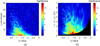 |
Fig. 4. Contour plots showing (a) significance vs. look ahead vs. k-value and (b) significance as a function of τ vs. k-value (where τ is obtained by multiplying the average waiting time based on that k-value by m). The lower boundary of this plot corresponds to m = 1 and also shows how the average waiting time depends on the k-value. The hashed region in the lower right is masked because we only analyze the mutual information for m ≥ 1. It is apparent that the information horizon detected between k = 0.6 and k = 2.4 appears to be consistent in duration (around 5 h), suggestive of an underlying dynamics that is independent of the threshold value. |
The increase in the number of events identified by reducing k also naturally decreases the mean waiting time of the distribution. To provide a perspective on the timescales involved, we multiplied the look ahead for a given threshold, m, by the average waiting time based on the threshold τ = m⟨Δ⟩ and then re-plotted panel a using τ instead of look ahead. As can be seen, the elevated significance appears to have a more uniform timescale (high significance lasts around 5 h), which suggests that there is a preferred timescale likely related to some physical process that is independent of the threshold. It should be noted that this timescale is similar to the timescale identified in the solar waiting time sequence (Snelling et al. 2020).
The mutual information is largest for successive flares m = 1; therefore, it is useful to examine the significance for successive flares as a function of threshold, k, as shown in Fig. 5. The significance increases as the threshold level is reduced and peaks around k = 1.56. For a lower threshold, there is a drastic reduction in significance, consistent with noise. These results are suggestive that a significant fraction of flare events normally discarded by taking a k = 3 threshold are, in fact, real events and not noise.
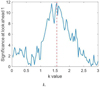 |
Fig. 5. Significance for successive flares as a function of threshold k. |
A simple experiment can be performed with the data to analyze the fraction of the light curve elevation events attributable to noise. As the peak information is found with k ≈ 1.56, we chose this threshold for the analysis; with this threshold we have 7213 events. To proceed, we randomly selected a percentage of these waiting times, which were each replaced by a waiting time randomly selected from the set of all the waiting times. This resampling procedure is known as bootstrapping. We then computed the mutual information of successive events (m = 1) for the data set that includes a percentage of bootstrapped data. As can be seen in Fig. 6, as the fraction of resampled values increases, the mutual information decreases. When 50% of the data have been resampled, it is no longer possible to detect any relationship between subsequent flares. Thus, it is clear that if the waiting times were randomly distributed, we would not find any significance. A similar result is found when k < 0.5, suggestive that there is legitimate noise in the light curves, but the high significance when k = 1.56 suggests that many of the events detected at this threshold reflect a dynamics that is significantly different than noise and may well be evidence of microflares.
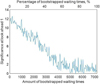 |
Fig. 6. Analysis of the fraction of the light curve elevation events from noise by bootstrapping. |
While this analysis suggests the existence of real flare events at low amplitude in the light curve of KIC 7985370, we can further explore whether the relationship detected by the mutual information results from flare clusters. If there are clusters of flares, it is likely that they occur in close temporal proximity to each other. We can systematically remove such flare events by introducing a minimum waiting time, Δmin. We then reexamined the waiting time sequence with the k = 1.56 selection criterion for which the mutual information is maximized. We analyzed the mutual information of successive events (m = 1) for a given value of Δmin. The significance is shown in Fig. 7. As can be seen, the significance decreases as Δmin increases until Δmin > 0.8 h, at which point it is no longer possible to determine any relationship between successive flares. This result suggests that the short-term memory mostly applies to flare waiting times that are less than 0.8 h. It should be noted, however, that this memory persists for about 5 h, as shown in Fig. 5.
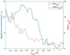 |
Fig. 7. Significance of successive events (m = 1) for a given value of Δmin (blue curve), and significance for a given value of Δmin if the decrease in significance is only a result of a decrease in the amount of data (dashed red curve). |
As mentioned previously, when there is a relationship between two random variables, the statistical significance generally increases with the number of events, as shown by Snelling et al. (2020). Thus, it is important to understand the extent to which the decrease in significance could be attributed to a decrease in the amount of data. As expected, when we impose a minimum flare waiting time (which effectively merges waiting times of less than Δmin), the total number of waiting times, N, decreases, as shown in Fig. 8 (panel a). The number of waiting times decreases from 7212 to around 175 when Δmin is equal to 1.16 h.
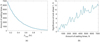 |
Fig. 8. Dependence of statistical significance on the amount of data, N. (a) N for a given value of Δmin. (b) Significance of successive events (m = 1) for a given value of N. |
As a second exercise, we calculated how the significance changes as we reduce the amount of data. Figure 8 (panel b) shows the significance of successive flares (m = 1) when only N waiting times are selected from the sequence for k = 1.56 (discarding the remaining 7212 N flares). As expected, the significance increases with N, and the relationship is linear when N is large.
Finally, we used the results from Fig. 8 to show how the significance would be expected to decrease with Δmin if the decrease only resulted from a decrease in the amount of data. This result was obtained by plotting the significance as a function of Δmin, using Fig. 8 (panel a) to find the amount of data, N, for the given value of Δmin and then using Fig. 8 (panel b) to obtain S(N(Δmin)). This curve is plotted in Fig. 7. It is apparent that the decrease in significance from Δmin = 0.1 h to Δmin = 0.7 h can be attributed to a reduction in the amount of data, but the decrease in significance from Δmin = 0.7 h to Δmin = 0.9 h can only be attributed to a change in the underlying dynamics. Figure 7 ultimately shows that the flares that violate a Poisson process are flares with a low waiting time. We therefore conclude that there is a distinct change in the dynamics of this class of events on timescales of less than 0.9 h. If we restrict our data set to flares with waiting times longer than 1 h, they could likely be modeled as a Poisson process; for waiting times of less than 1 h, this is not possible.
4. Limitations of noise thresholding methods for the detection of flares and possible solutions
The conventional application of a threshold condition to the detrended light curves of stars certainly seems appropriate for differentiating flare events from noise. Stellar variability, instrumental fluctuations, and shot noise likely form the major noise components in the system. The conventional approach is to assume that the amplitude of the noise distribution is characterized by its standard deviation, σ, and the noise threshold is then set at kσ, where k > 0. As we have shown, below some threshold level, the information in the trend-less light curve of the solar-type star KIC 7985370 is dominated by noise.
However, the k-σ approach for flare detection purposes in light curves uses a rule of thumb basis to choose a certain value of k and therefore requires a certain level of expertise. Also, a subsequent visual inspection is often needed to verify the accuracy of the detection (Vida & Roettenbacher 2018; Oláh et al. 2021). However, this empirical procedure is not always justified and could produce results that can cause many real flares to go unidentified or discarded. Light curves may contain significant but low flare-to-noise ratio peaks that may be scattered among much more intense peaks. These peaks will be lost at the thresholding stage if the actual noise level is overestimated by the kσ value. Also, as light curve data sets become ever greater, as in the case of the analysis of ensembles of stars (Maehara et al. 2012; Davenport 2016), it can become increasingly impractical to use the rule of thumb basis to obtain the same quality of results as can be accomplished when analyzing only a data set from a star. Given the difficulties associated with the k-σ standard approach, where the statistical distribution for noise is defined in order to identify flares, another approach that provides a robust and reliable identification of flares is needed.
Although information theory has been applied to a large number of problems in the studies of solar and space physics (Johnson & Wing 2005, 2014; Johnson et al. 2018; Wing & Johnson 2019; Wing et al. 2005, 2016, 2018, 2020, 2022; Rivera et al. 2022), so far as we know, it has not been used as a means of proposing a thresholding method for stellar flare detection. To maximize the return from the light curve data, it may be useful to consider a new thresholding method based on this study for the detection of flare events. In this method, the value of k would be determined so as to maximize the significance of the mutual information contained in the flare sequence. That is, the short-term memory evident both in the Sun and in other stars, such as KIC 7985370, can be used to identify the transition from flare dynamics to shot noise. In the case of KIC 7985370, it appears that 50% of the k = 1.56 threshold events exhibited characteristics different from noise.
5. Conclusions
In this paper we have analyzed the light curve of KIC 7985370. Flare events were identified from the detrended light curve as excursions above a kσ threshold value. We examined how the choice of the threshold, k, affects the information content of the flare sequence. The study uses a theoretical information approach that takes advantage of the additional information encoded in the ordering of a time sequence. Our analysis of this star shows:
-
When the light curve over the entire period is considered, we see that there is an optimal threshold level (kσ) when k is 1.56, showing that even with a threshold around 1.56σ the dynamics of the flare events are dramatically different from the dynamics of shot noise. This elevated significance suggests a short-term memory between events and is similar to our analysis of the solar waiting time sequence (Snelling et al. 2020).
-
When a fraction of the waiting times are resampled using a bootstrap method (Fig. 6), we find that we could eliminate the memory by shuffling 50% of the waiting times randomly, suggesting that about 50% of the noise may be actual flare events.
-
When we considered the timescale on which successive flares are related, we found that the short-term memory is eliminated when all flare waiting times lower than a given Δmin are merged. This result suggests that, for KIC 7985370, there are clusters of flare events that occur with a time separation of less than 1.5 h. These timescales are similar to (although slightly shorter than) the timescale on which solar flares are related (Rivera et al. 2022).
These results suggest that an information-theory-based threshold that maximizes the information contained in the flare sequence may detect a more complete stellar flare candidate list by better capturing the real information contained in a light curve. In addition, it minimizes the number of noise peaks included, thus reducing the proportion of false positives. In practice, the method can outperform noise-based flare detection methods by maximizing the significance of mutual information to determine the optimal threshold level. This procedure is fast enough to work within existing workflows with large amounts of data. It should also be noted that the method could be extendable to any form of signal processing application for peak detection.
Acknowledgments
This work is supported by NASA grants NNX16AQ87G, 80NSSC21K1678, 80NSSC20K0355, 80NSSC20K0704, 80NSSC22K0515, and NSF AGS grant 2131013.
References
- Aerts, C., Christensen-Dalsgaard, J., & Kurtz, D. W. 2010, Asteroseismology (New York: Springer Science& Business Media) [Google Scholar]
- Aschwanden, M. J., & Johnson, J. R. 2021, ApJ, 921, 82 [NASA ADS] [CrossRef] [Google Scholar]
- Aschwanden, M. J., & McTiernan, J. M. 2010, ApJ, 717, 683 [NASA ADS] [CrossRef] [Google Scholar]
- Balona, L., Pigulski, A., Cat, P. D., et al. 2011, MNRAS, 413, 2403 [NASA ADS] [CrossRef] [Google Scholar]
- Berdyugina, S. V. 2005, Liv. Rev. Sol. Phys., 2, 8 [Google Scholar]
- Borucki, W. J., Koch, D., Basri, G., et al. 2010, Science, 327, 977 [Google Scholar]
- Davenport, J. R. 2016, ApJ, 829, 23 [NASA ADS] [CrossRef] [Google Scholar]
- Deco, G., & Schhurmann, B. 2000, Information Dynamics: Foundations and Applications (Berlin: Springer-Verlag) [Google Scholar]
- Fabbian, D., Simoniello, R., Collet, R., et al. 2017, Astron. Nachr., 338, 753 [NASA ADS] [CrossRef] [Google Scholar]
- Feinstein, A. D., Montet, B. T., Ansdell, M., et al. 2020, AJ, 160, 219 [Google Scholar]
- Fröhlich, H. E., Frasca, A., Catanzaro, G., et al. 2012, A&A, 543, A146 [CrossRef] [EDP Sciences] [Google Scholar]
- Hannah, I., Hudson, H., Battaglia, M., et al. 2011, Space Sci. Rev., 159, 263 [NASA ADS] [CrossRef] [Google Scholar]
- Johnson, J. R., & Wing, S. 2005, J. Geophys. Res. (Space Phys.), 110, A04211 [NASA ADS] [Google Scholar]
- Johnson, J. R., & Wing, S. 2014, Geophys. Res. Lett., 41, 5748 [NASA ADS] [CrossRef] [Google Scholar]
- Johnson, J. R., & Wing, S. 2018, in Machine Learning Techniques for Space Weather, eds. E. Camporeale, S. Wing, & J. R. Johnson (Elsevier), 45 [CrossRef] [Google Scholar]
- Johnson, J. R., Wing, S., & Camporeale, E. 2018, Ann. Geophys., 36, 945 [NASA ADS] [CrossRef] [Google Scholar]
- Li, C., Zhong, S., Xu, Z., et al. 2018, MNRAS, 479, L139 [NASA ADS] [CrossRef] [Google Scholar]
- Maehara, H., Shibayama, T., Notsu, S., et al. 2012, Nature, 485, 478 [NASA ADS] [Google Scholar]
- Mossoux, E., & Grosso, N. 2017, A&A, 604, A85 [NASA ADS] [CrossRef] [EDP Sciences] [Google Scholar]
- Nurhan, Y. I., Johnson, J. R., Homan, J. R., Wing, S., & Aschwanden, M. J. 2021, Geophys. Res. Lett., e2021GL094348 [Google Scholar]
- Oláh, K., Kővári, Z. S., Günther, M., et al. 2021, A&A, 647, A62 [NASA ADS] [CrossRef] [EDP Sciences] [Google Scholar]
- Reinhold, T., Reiners, A., & Basri, G. 2013, A&A, 560, A4 [NASA ADS] [CrossRef] [EDP Sciences] [Google Scholar]
- Rivera, E. C., Johnson, J. R., Homan, J., & Wing, S. 2022, ApJ, 937, L8 [NASA ADS] [CrossRef] [Google Scholar]
- Shibayama, T., Maehara, H., Notsu, S., et al. 2013, ApJS, 209, 5 [Google Scholar]
- Snelling, J. M., Johnson, J. R., Willard, J., et al. 2020, ApJ, 899, 148 [NASA ADS] [CrossRef] [Google Scholar]
- Stelzer, B., Damasso, M., Scholz, A., et al. 2020, A&A, 637, A22 [NASA ADS] [CrossRef] [EDP Sciences] [Google Scholar]
- Strassmeier, K. G. 2009, A&ARv, 17, 251 [Google Scholar]
- Vida, K., & Roettenbacher, R. M. 2018, A&A, 616, A163 [NASA ADS] [CrossRef] [EDP Sciences] [Google Scholar]
- Wheatland, M., & Litvinenko, Y. E. 2002, Sol. Phys., 211, 255 [NASA ADS] [CrossRef] [Google Scholar]
- Wing, S., & Johnson, J. R. 2019, Entrp, 21, 140 [NASA ADS] [CrossRef] [Google Scholar]
- Wing, S., Johnson, J., Jen, J., et al. 2005, J. Geophys. Res. (Space Phys.), 110 [Google Scholar]
- Wing, S., Johnson, J. R., Camporeale, E., & Reeves, G. D. 2016, J. Geophys. Res. (Space Phys.), 121, 9378 [NASA ADS] [CrossRef] [Google Scholar]
- Wing, S., Johnson, J. R., & Vourlidas, A. 2018, ApJ, 854, 85 [NASA ADS] [CrossRef] [Google Scholar]
- Wing, S., Brandt, P., Mitchell, D., et al. 2020, ApJ, 159, 249 [CrossRef] [Google Scholar]
- Wing, S., Johnson, J. R., Turner, D. L., Ukhorskiy, A. Y., & Boyd, A. J. 2022, J. Geophys. Res. (Space Phys.), 127, e2021JA030246 [Google Scholar]
- Yang, H., & Liu, J. 2019, ApJS, 241, 29 [NASA ADS] [CrossRef] [Google Scholar]
- Yang, H., Liu, J., Gao, Q., et al. 2017, ApJ, 849, 36 [NASA ADS] [CrossRef] [Google Scholar]
- Yang, H., Liu, J., Qiao, E., et al. 2018, ApJ, 859, 87 [NASA ADS] [CrossRef] [Google Scholar]
All Figures
|
Fig. 1. Light curve for KIC 7985370. (a) Application of our flare selection criteria applied to the data with k = 1.56; flare events are shown as open orange circles. (b) Zoomed-in view of the group of flares in the red shaded box. |
| In the text | |
|
Fig. 2. Waiting time distribution for the entire period and stationary Poisson distribution (p ∝ 0.2423e−1.373Δ). |
| In the text | |
|
Fig. 3. Information content as a function of look ahead, m. (a) Mutual information with k-threshold equal to 2. Mutual information of 50 surrogates is shown as a green line, and the envelope of the 3σ the fluctuation of the surrogates is shaded yellow. Note that the look ahead axis begins at m = 1. (b) Significance of the mutual information as a function of look ahead. The significance is elevated for m = 1 and 2, indicating that successive flares have a relationship. |
| In the text | |
|
Fig. 4. Contour plots showing (a) significance vs. look ahead vs. k-value and (b) significance as a function of τ vs. k-value (where τ is obtained by multiplying the average waiting time based on that k-value by m). The lower boundary of this plot corresponds to m = 1 and also shows how the average waiting time depends on the k-value. The hashed region in the lower right is masked because we only analyze the mutual information for m ≥ 1. It is apparent that the information horizon detected between k = 0.6 and k = 2.4 appears to be consistent in duration (around 5 h), suggestive of an underlying dynamics that is independent of the threshold value. |
| In the text | |
|
Fig. 5. Significance for successive flares as a function of threshold k. |
| In the text | |
|
Fig. 6. Analysis of the fraction of the light curve elevation events from noise by bootstrapping. |
| In the text | |
|
Fig. 7. Significance of successive events (m = 1) for a given value of Δmin (blue curve), and significance for a given value of Δmin if the decrease in significance is only a result of a decrease in the amount of data (dashed red curve). |
| In the text | |
|
Fig. 8. Dependence of statistical significance on the amount of data, N. (a) N for a given value of Δmin. (b) Significance of successive events (m = 1) for a given value of N. |
| In the text | |
Current usage metrics show cumulative count of Article Views (full-text article views including HTML views, PDF and ePub downloads, according to the available data) and Abstracts Views on Vision4Press platform.
Data correspond to usage on the plateform after 2015. The current usage metrics is available 48-96 hours after online publication and is updated daily on week days.
Initial download of the metrics may take a while.