| Issue |
A&A
Volume 670, February 2023
Solar Orbiter First Results (Nominal Mission Phase)
|
|
|---|---|---|
| Article Number | A140 | |
| Number of page(s) | 18 | |
| Section | Planets and planetary systems | |
| DOI | https://doi.org/10.1051/0004-6361/202245165 | |
| Published online | 20 February 2023 | |
Modeling Solar Orbiter dust detection rates in the inner heliosphere as a Poisson process
1
Department of Physics and Technology, UiT The Arctic University of Norway,
9037
Tromsø, Norway
e-mail: This email address is being protected from spambots. You need JavaScript enabled to view it.
2
Department of Mathematics and Statistics, UiT The Arctic University of Norway,
9037,
Tromsø, Norway
3
LESIA, Observatoire de Paris, Université PSL, CNRS, Sorbonne Université, Université de Paris,
Paris, France
Received:
7
October
2022
Accepted:
3
January
2023
Abstract
Context. Solar Orbiter provides dust detection capability in the inner heliosphere, but estimating physical properties of detected dust from the collected data is far from straightforward.
Aims. First, a physical model for dust collection considering a Poisson process is formulated. Second, it is shown that dust on hyperbolic orbits is responsible for the majority of dust detections with Solar Orbiter’s Radio and Plasma Waves (RPW). Third, the model for dust counts is fitted to Solar Orbiter RPW data and parameters of the dust are inferred, namely radial velocity, hyperbolic meteoroids predominance, and the solar radiation pressure to gravity ratio as well as the uncertainties of these.
Methods. Nonparametric model fitting was used to get the difference between the inbound and outbound detection rate and dust radial velocity was thus estimated. A hierarchical Bayesian model was formulated and applied to available Solar Orbiter RPW data. The model uses the methodology of integrated nested Laplace approximation, estimating parameters of dust and their ncertainties.
Results. Solar Orbiter RPW dust observations can be modeled as a Poisson process in a Bayesian framework and observations up to this date are consistent with the hyperbolic dust model with an additional background component. Analysis suggests a radial velocity of the hyperbolic component around (63 ± 7) km s−1 with the predominance of hyperbolic dust being about (78 ± 4)%. The results are consistent with hyperbolic meteoroids originating between 0.02 AU and 0.1 AU and showing substantial deceleration, which implies effective solar radiation pressure to a gravity ratio ≳ 0.5. The flux of the hyperbolic component at 1 AU is found to be (1.1 ± 0.2) × 10−4 m−2s−1 and the flux of the background component at 1 AU is found to be (5.4 ± 1.5) × 10−5 m−2s−1.
Key words: zodiacal dust / methods: statistical
© The Authors 2023
 Open Access article, published by EDP Sciences, under the terms of the Creative Commons Attribution License (https://creativecommons.org/licenses/by/4.0), which permits unrestricted use, distribution, and reproduction in any medium, provided the original work is properly cited.
This article is published in open access under the Subscribe to Open model. This email address is being protected from spambots. You need JavaScript enabled to view it. to support open access publication.
1 Introduction
Among dust detected with in situ measurements within 1 AU, particles on unbound hyperbolic trajectories originating in the relative vicinity of the Sun play a major role, as has already been shown in the case of measurements of Solar Orbiter (Zaslavsky et al. 2021). Most of these hyperbolic particles of a submicron size are believed to be so-called β meteoroids, which are generated by a high radiation pressure to gravity ratio, denoted as β:
 (1)
(1)
It is clear that in the region of dust sizes s ≫ λ ≈ 500 nm, where s denotes the dimension of a dust particle and λ denotes the wavelength of incident light, Fradiation depends on a dust particle’s cross section, while Fgravity depends on a dust grain’s volume. Hence, the smaller the particle, the higher the β value. A maximum of β is therefore reached when s ≈ λ and usually βmax ≈ 1. Notably, both Fradiation and Fgravity depend on the inverse square of heliocentric distance, hence β remains constant for a given particle throughout its trajectory. We note that Fradiation and Fgravity are the predominant forces for the β meteoroids, as electromagnetic forces become relevant for dust grains of size s < 100 nm (Mann et al. 2014). Dust of size s < 100nm can also be on an unbound trajectory due to electromagnetic forces (Czechowski & Mann 2021; Mann & Czechowski 2021).
For β = 1, the grain neither accelerates nor decelerates due to Solar influence. For β = 0.5, the grain feels solar attraction, but effective Solar attraction is reduced to one-half, which means that a sudden change in β from 0 to 0.5, for example due to a change in the size of the grain, causes an originally circular orbit to become an unbound, parabolic orbit. Particles with β ≥ 0.5 are created mostly in collisions of larger dust (Dohnanyi 1972, Zook & Berg 1975, and Grün et al. 1985). Larger particles have very low β ≪ c 1 and are therefore originally on Keplerian orbits (referred to as initial orbits hereafter), hence β = 0.5 could be considered the minimal value needed for dust to become unbound.
The population of bound (β ≪ 0.5) dust particles inside 1 AU is notably responsible for visual observations of zodiacal light. Their spatial density has been observed to depend on heliocen tric distance approximately as ~r–1.3 (Leinert et al. 1981), which holds well down to 20 R⊙, or 0.1 AU. Inward of that distance, they show shallower dependence, suggesting a maximum in density somewhere inward of 0.05 AU, or 10 R⊙ (Stenborg et al. 2021). Regions with high density of bound dust is very likely the region of origin of β meteoroids, as the collision rate of bound dust depends on the square of its spatial density (Mann & Czechowski 2005).
As β meteoroids likely make up most of the submicron hyperbolic dust where the particles considered have sizes s > 100 nm, the two terms are almost interchangeable for the purpose of the present discussion (Zaslavsky et al. 2021). The term β meteoroids is used where radiation pressure ejection is important and the term hyperbolic dust is used where only trajectories of the grains are relevant.
The detection of bound dust particles is usually done remotely, both historically (Van de Hulst 1947 and Leinert et al. 1981) and currently (Howard et al. 2019 and Stenborg et al. 2021), taking advantage of light scattering properties of these particles. The detection of submicron particles is done mostly in situ (at an encounter with a particle), due to their insignificant light scattering properties and low spatial density, often taking advantage of the so-called impact ionization effect (Fri-ichtenicht 1962 and Alexander & Bohn 1968). Impact ionization dust detection is a passive data-gathering process carried out by either a specialized instrument (Dietzel et al. 1973 and Srama et al. 2004) or often as a byproduct of electric (Gurnett et al. 1997; Meyer-Vernet et al. 1986; Kurth et al. 2006; Wang et al. 2006; Zaslavsky et al. 2012, 2021; Vaverka et al. 2018; Malaspina et al. 2020; Mozer et al. 2020; and Nouzk et al. 2021) or magnetic (Malaspina et al. 2022 and Gasque et al. 2022) measurements. Due to high energy density present at the impact site, free charge is generated upon a hypervelocity dust impact. The charge generated is partially picked up by the spacecraft body and/or antennas, which results in specific signatures in fast electric measurements (Zaslavsky 2015; Meyer-Vernet et al. 2017; Vaverka et al. 2017; Mann et al. 2019; Shen et al. 2021; Rackovic Babic et al. 2022). The amount of generated charge Q has been empirically found to approximately follow the equation
 (2)
(2)
where in the range of impact velocities 20 km s−1 < v < 50 km s−1 achieved in laboratory (Friichtenicht 1962; Dietzel et al. 1972; and Shu et al. 2012) γ ≈ 1 and 3 ≲ a ≲ 5. All three parameters A, γ, and α are dependent on both the material of the grain and the target (Grün 1984; Grün et al. 2007; and Collette et al. 2014).
For many decades now, it has been standard to express cumulative mass distribution of dust near 1 AU in terms of a power-law distribution over about 20 decades of masses, from nanodust to comets and asteroids and above. Clearly, the distribution is an approximation and the distribution is described with a different exponent in different intervals. However, it is often the case that a single experiment is sensitive over several orders of magnitude and finds that the mass distribution (number of particles with a mass of at least m) follows a power-law
 (3)
(3)
over the observed range. For example, the work of Whipple (1967) reported δ ≈ 1.34 for the mass range 10−8–10−1 kg and δ ≈ 0.51 for the mass range 0−13–10−8kg. Compiling previous estimates and relying on the stationarity of a dust cloud, Dohnanyi (1970) reported δ ≈ 7/6 for sporadic meteoroids of masses from macroscopic down to 10−11 kg and δ ≈ 1/2 between 10−14kg and 10−11kg. Grün et al. (1985) suggested δ ≈ 0.8 in the range 10−21–10−17 kg, that is β meteoroids and smaller. Recently, Zaslavsky et al. (2021) inferred δ ≈ 0.34 for Solar Orbiter’s Radio and Plasma Waves (RPW) dust detections of dust of m ≳ 10−17 kg. It is not clear whether Eq. (3) represents a good approximation for β meteoroids.
A Poisson point process is a stochastic process defined by the following properties: (1) a Poisson distribution of counts within an arbitrarily chosen bounded region (for example a temporal interval); (2) statistical independence of counts within disjoint regions (temporal intervals); and (3) no two events can happen at the exact same location (time).
It is reasonable to assume that the third condition is met, especially near 1 AU. For Solar Orbiter specifically, the detection of two subsequent impacts is possible unless they happened in the same 62 ms window, which is unlikely given the mean waiting time ≈200 s on the most hit intensive days (see Fig. 4). The first two conditions demand that a detection of a dust particle does not influence the probability of detection of a particle at any other point in time, for example particles do not interact, and their reservoir cannot be depleted. In the case of β meteoroids, all of these can be assumed, as particles are likely formed far away from the spacecraft, they are sparsely distributed, and their trajectories are uncorrelated. We are aware that the Solar System’s dust cloud is not homogeneous on small scales and that a large stream (Szalay et al. 2021) or a coronal mass ejection (Ragot & Kahler 2003) could alter the rate on short timescales, but we see no evidence for that with Solar Orbiter. Therefore, a Poisson process is the simplest conceivable model and it is natural to consider dust counts as an inhomogeneous Poisson point process, that is a Poisson process with a nonconstant rate. This means that the rate depends on other parameters, in our case the distance from the Sun and spacecraft velocity. In fact, the observed number of detections within a naturally considered temporal interval, for example an hour or a day, is usually a low number. This implies a considerable probability of zero detections, which makes the random variable of detections per temporal interval a poor fit to a frequently considered normal distribution, which allows for negative numbers. Hence, a Poisson distribution of counts should be considered.
Inferring the variable detection rate could be done by least squares fitting a model onto a time series of detections per unit time, as is often done. A least squares fit produces the maximum likelihood estimate when the error of the data (residuals) are normally distributed. However, detections per unit time have a Poisson distribution, as discussed above. It is possible to obtain a maximum likelihood estimate with more careful analysis, but uncertainty is not directly accessible and must be estimated by other means (for example using the bootstrap method). Adapting a procedure designed specifically to fit a Poisson process to Poisson observations grants the resolution needed to fit a complicated model precisely. Moreover, given we meet model assumptions, we can make more meaningful error estimates and potentially compare competing models in a meaningful way.
In the present work, we take advantage of the Bayesian inference, which is a general procedure that works with models for observations with unknown parameters and meets both of the above-mentioned criteria: it handles the Poisson distribution and provides an uncertainty estimate. In this approach, unknown parameters are regarded as random variables coming from an unknown distribution, about which some prior information is available (in the form of a prior belief, or prior distribution). The procedure infers the posterior (improved) distribution of unknown parameters based on the prior distribution and observed data. This distribution automatically carries information about uncertainty.
Integrated nested Laplace approximation (Rue et al. 2009, 2017; INLA for short) implements an approximate Bayesian inference for a wide class of three-stage hierarchical models. This class of models contains multilevel (nested) models, spatio-temporal models, survival models, and others (Gómez-Rubio 2020). A decisive advantage of INLA as opposed to other Bayesian methods (for example sampling-based methods) is its computational efficiency allowing for one to fit more complicated models to more observations within available time, making it the method of choice for the course of this work. The inference is carried out using the R-INLA package (Martins et al. 2013 and Rue et al. 2017) for the Bayesian inference.
In Sect. 2, we briefly introduce the Solar Orbiter mission, its dust measurement results, and the data product that we use throughout the work. Section 3 is a discussion and analysis of observed hyperbolic dust velocity. The fitting of the dust detection rate using INLA is presented in Sect. 4 and we conclude our findings in Sect. 5. Finally, an outlook for Solar Orbiter and other missions is briefly discussed in Sect. 6.
2 Solar Orbiter’s dust observations and data products
Solar Orbiter is a spacecraft that orbits the Sun on an elliptical trajectory. Solar Orbiter underwent several gravity assists and its orbital parameters have therefore changed several times since its launch in early 2020. As of the summer of 2022, Solar Orbiter has had a low inclination, effectively making measure ments in the ecliptic plane. Its aphelion is close to 1 AU and perihelion 0.3 AU; however, for the majority of its mission so far, its perihelion has been close to 0.5 AU.
Radio and Plasma Waves (RPW) is an experiment onboard Solar Orbiter designed to measure both the electric and the magnetic field in three components in a wide frequency band, from near-DC to 16 MHz in the case of the electric field (Maksimovic et al. 2020). The measurements of electric fields, and as is crucial for the present work, allow for the detection of cosmic dust impacts, which is one of the auxiliary scientific objectives of Solar Orbiter. A part of the data analyzed here was accessed at Solar Orbiter/RPW Investigation (2022)1, specifically time domain sampler (TDS) waveform electrical data (Level 2).
In their recent work, Zaslavsky et al. (2021) describe properties of Solar Orbiter’s RPW as a dust detector. It has the capacity of C ≈ 250 pF, a sensitivity to pulses of V ≳ 5 mV, a collection area of Scol ≈ 8 m2, and a duty cycle of D ≈ 6.2%. They show that Solar Orbiter’s RPW instrument is indeed capable of dust detections and that these could be modeled as hyperbolic dust. The authors mostly discuss β meteoroids, as they are likely the observed population, but in principle the model fits to any hyperbolic dust population. The model for the detection rate R presented in the aforementioned work,
 (4a)
(4a)
 (4b)
(4b)
has three parameters: αδ, F1AUScol, and υdust. We note that, both αδ, and F1 AUScol are products of two quantities. All three parameters could have a spatio-temporal dependence.
The model shows a good fit to the data with the parameters that are considered constant: the outward radial heliocentric speed of υdust ≈ 50 km/s and exponent αδ ≈ 1.3. The value for υβ was inferred by relating the difference in the detection rate in the inbound and the outbound leg of an orbit (Zaslavsky et al. 2021) and it was used directly, not as a free parameter of Eq. (4a). A value of δ ≈ 0.34, which is a dimensionless parameter in mass distribution of detected dust grains (see Eq. (3)), was inferred from the distribution of impact pulse amplitudes. The value of α, which stands for the power of velocity in charge-yield Eq. (2) is deduced from the knowledge of αδ and δ. It is important to note that a is often measured in a laboratory setup and its inferred value is compatible with ground-based measurements (Collette et al. 2014). The exponent of αδ accounts for the change in sensitivity due to higher velocity, hence the flux is to be hereafter understood as the flux of detectable grains or the flux of grains that are large and fast enough. The parameter F1AU stands for the flux at 1 AU, F1 AU ≈ 8 × 10⁻⁵ m−2 s−1 (see Zaslavsky et al. 2021 for details).
In addition to L2 Solar Orbiter RPW data, this work makes use of the data product provided by Kvammen et al. (2023), which is a result of a convolutional neural-network-classified time-domain-sampled data. It builds on a supervised classification algorithm trained using a randomly chosen subsample of manually labeled data. Its main advantage over visual inspection of all data on-board classified as dust (which is a time-consuming task) is that it is fully automatic and reasonably time-consuming. Therefore, it allows for not only type 1 error correction (detection confirmation), but also for type 2 error correction, implying a search for dust in the vast data that has not been classified as dust by an on-board algorithm a priori. Building upon the analysis of TDS snapshots, it is worth mentioning that the classifier distinguishes impacts happening in distinct snapshots, but it is not reliable with the detection of two impacts within the same snapshot, which is an unlikely situation. There is also a necessary amplitude filter, as only transmitted TDS snapshots could be classified, while only snapshots containing phenomena of a sufficient amplitude are transmitted. This however does not spoil the assumption of Poisson distribution and it is accounted for in the analysis. Although no supervised classifier could get rid of human bias and error completely, these data provide the most reliable Solar Orbiter dust detection data available to date, as has been shown in Kvammen et al. (2023). The data set consists of 4606 dust detections acquired over approximately 669 h within 457 days between 29 June 2020 and 16 December 2021.There are several intervals of unavailable data lasting longer than a week in July and August of 2020 (23 days) and September of 2021 (9 days). We make use of the data that were publicly available on 01 September 2022. We refer to these data as TDS/TSWF-E/CNN and it is publicly accessible (see Kvammen et al. 2023).
3 Impact rates and velocities of hyperbolic dust
3.1 Single-particle velocities
We note that β meteoroids are moving mostly radially outward from their region of origin, which is located well within 0.5 AU. Figures 1, 2 display possible single-particle velocity profiles (see Appendix A for underlying equations). As β < 0.5 leads to finite aphelion, β ≈ 1 requires a rather specific set of parameters, and values of β ≳ 0.5 are shown. We note that this choice is inconsequential and was made for illustration purposes only, as we do not presuppose a β value in a further analysis. In fact, we do not presuppose that the observed population includes β meteoroids, though that is likely the case. The effective initial orbit of β grain’s parent body must lie outside of the near-solar dust-free zone, but in the region with a high bound dust concentration, which restrains the r0 values shown. As shown in Fig. 1, radial β meteoroid velocities expected between 0.5 AU and 1 AU are between 30 km s−1 and 90 km s−1 for the given combinations of parameters and they are nearly independent of heliocentric distance (nearly constant). Solar gravity and radiation pressure forces are central forces; therefore, the β value does not influence azimuthal velocity as a function of heliocentric distance, which is governed by angular momentum conservation and the initial orbit only. Azimuthal velocities of β meteoroids of chosen parameters between 0.5 AU and 1 AU are therefore between 7 km s−1 and 30 km s−1 and decreasing ∝ r–1, as shown in Fig. 2.
If dust detections on Solar Orbiter’s RPW correspond to hyperbolic dust, a difference in detection rate Rin versus Rout due to spacecraft radial velocity should be present, as is indeed the case. It is shown by Zaslavsky et al. (2021) that this approach allows for an order of magnitude estimation of the radial compo nent of dust velocity υdust;rad ≈ 50 km s−1, which is in line with expectations. In the present work, we extend the approach to estimate continuous heliocentric-distance-dependent dust radial velocities, using the data product of Kvammen et al. (2023) and taking into account more unknown variables that influence our estimates.
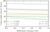 |
Fig. 1 Radial velocity profiles of β meteoroids released by a sudden parameter change (for example due to a collision) from an initially cir cular orbit. A selection of β values and origins (r0) is shown. |
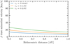 |
Fig. 2 Azimuthal velocity profiles of β meteoroids released by a sudden parameter change (for example, due to a collision) from an initially circular orbit. A selection of origins (r0) is shown, with the β value not being relevant. |
3.2 Velocity estimation
A first estimate of υdust;rad is obtained if a model for the dust collection rate with linear dependence on relative Solar Orbiter and dust velocity υimpact is assumed (R ∝ υimpact). This corresponds to linear dependence on the volume of space scanned per unit of time only:
 (5)
(5)
where  is the absolute value of the spacecraft’s radial velocity at a given heliocentric distance. We note that Rin and Rout are obtained at the same heliocentric distance, but in inbound and outbound legs of the orbit, respectively. If, however, a different dependence of R (vimpact) is assumed, Eq. (5) changes. Assuming R ∝ υimpact, a second estimate of υdust;rad is obtained by
 (6a)
(6a)
 (6b)
(6b)
where q is equivalent to 1 + αδ in Eq. (4a) and  has no direct physical interpretation. We took the spacecraft’s azimuthal velocity into account, but not the dust’s azimuthal velocity, as that would be a second unknown component for which we do not have enough information. It is nonetheless possible to correct for assumed dust azimuthal velocity by subtracting it from υsc (see Appendix B for the derivation of Eqs. (5)-(6b)).
It follows from Eq. (6a) that with Rin and Rout being observed, the value of q > 1 leads to a higher velocity estimate than in the case of q = 1, an estimate that is higher by a factor of q in first order approximation. Zaslavsky et al. (2021) reported inferred velocities υdust;rad ≈ 50 km/s assuming q = 1 and they show compatibility of detection rates with the model assuming q = 1 + αδ ≈ 2.3 according to Eq. (4a). With assumptions being met, υdust;rad ≈ 50 km/s is likely an underestimate. The most important assumption here is that the dust does indeed come from a hyperbolic population.
We note that the assumption that all detected dust grains are hyperbolic is difficult to verify or falsify. The most prominent trend in detections is that the counts diminish with increasing heliocentric distance, which could easily hide a plethora of other components, such as bound dust or interstellar dust. The first correction to the assumption that all detections come from a hyperbolic dust stream is the assumption of having a two-component field: hyperbolic dust and sporadic (back ground) detections, with the latter having no dependence on the spacecraft location or velocity. This is not to say that the nonhy-perbolic component has no temporal dependence, this is just the simplest conceivable correction. For further discussion, readers can refer to Sect. 4.4.
3.3 Velocity inference
Assuming that the dust flux is not explicitly dependent on time, the dust detection rate is a function of orbital phase as long as the orbital parameters do not change. Conversely, gravity assists change orbital parameters, such as perihelion, aphelion, and eccentricity. For the present analysis, we therefore treated sets of orbits, delimited by gravity assists, as separate data sets. In this way, data were aggregated for several orbits with the same orbital parameters, but we did not aggregate incompatible measurements. For instance, dust detection counts recorded near 0.6 AU on branches 2 and 3 are expected to be very different due to a vastly different Solar Orbiter radial velocity (see Solar Orbiter’s radial velocity and its heliocentric location throughout its trajectory in Fig. 3). Minor orbital alterations between gravity assists have been neglected.
Since 29 June 2020, Solar Orbiter has undergone three gravity assists, producing four distinct sets of data. The last of these chronologically so far did not accumulate data sufficient for analysis, and crucially did not produce any detections in the inbound part of the orbit at the time of analysis, hence the first three branches were used. The difference between a detection rate in the inbound and outbound leg of an orbit could be used for dust radial velocity inference, provided that radial spacecraft velocity is not negligible, compared to dust radial speed. Hence data represented by dashed lines in Fig. 3 are not used for this analy sis. Data with radial spacecraft velocity < 5 km s−1 are not used as they carry little information (see horizontal dashed line in Fig. 3).
In order to estimate radially dependent velocity, we produced smooth estimates of radially dependent detection rates, as defined in the TDS/TSWF-E/CNN data set. The fitting was done separately for inbound and outbound legs for each gravity assist delimited data set. In order to not rely on assumptions, we decided to use nonparametric fitting, specifically Nadaraya-Watson kernel regression (Watson 1964 and Nadaraya 1964) with a Gaussian kernel (FWHM ≈ 2.355σ = 0.15 AU). This is a simple and robust local-averaging fitting procedure, producing C∞ estimates. Dust detection counts are Poisson random variables; therefore, they have a variance equal to their mean value. To evaluate the uncertainty, we constructed confidence intervals for the nonparametric fit by bootstrapping on daily dust counts: new samples were generated with original counts as rates for new Poisson-distributed random variables. For an illustration of all three data sets and fitted rates, readers can refer to Fig. 4. It is important to keep in mind that the detection rates here after have been normalized to the observation time. For every branch, we only used the heliocentric distance interval where both inbound and outbound legs are available, bounded by the innermost and the outermost detection on the leg (see the grayed areas in Fig. 4). We did not use the r < 0.62 AU of branch 2, as there are no outbound detections near 0.6 AU and the detections near 0.5 AU show little difference between the inbound and the outbound leg. This may be due to a spatial limitation of the given model, an unlikely combination due to scarce data, a truly higher radial velocity, or a combination of more effects.
Having smooth detection rate estimates, we produced velocity estimates using Eq. (6a) (see Fig. 5). Bootstrap samples of detection rates were used to calculate the shown percentile confidence intervals. Notably, not all the bootstrap samples for λbg = 4 h−1 allowed for a solution, which is apparent from the jitters of the blue curve at r > 0.75 AU. Confidence intervals were constructed from the solutions that were obtained. This issue is to be expected, as λbg = 4 h−1 implies very little hyperbolic dust at r > 0.8 AU (see Fig. 4) and therefore uncertainty in the inferred velocity. The estimate shown in Fig. 5 assumes αδ = 1.3 and an initial heliocentric distance of 0.1 AU, with the latter in the form of correction for dust azimuthal velocity.
To further estimate the uncertainty, we included three relevant parameters (in total): (1) a background (nonhyperbolic) rate λbg, corrected for by subtraction from the estimated detection rate; (2) the product αδ included in Eq. (6a); and (3) azimuthal dust velocity corresponding to different initial circular orbits, as shown in Fig. 2, giving a straightforward generalization of Eq. (6a).
We have an estimate of the region of likely velocities (see Fig. 6), given a reasonable variation of free parameters. The analysis shows the velocity to be mostly between 40 km s−1 and 100 km s−1, according to Fig. 6. We know that the rate λbg of constant, nonhyperbolic dust could clearly not be lower than 0 and could not be much higher than ≈4 h−1 either, because the total detection rate is about ≈ 4 h−1 at a heliocentric distance ≈ 1 AU, which would imply 100% contribution of background dust in this region (see Fig. 4). This explains why no solutions of Eq. (6a) are found near 1 AU in that case, as Fig. 5 shows. The reason being that the difference between inbound and outbound rates are observed to be too high, such that they cannot be explained in the case of λbg = 4 h−1. λ rather low amount (≲1 h−1) of non-hyperbolic dust would imply a higher velocity in the range of ≈100 km s−1. The conclusion is that the higher the background detection rate λbg is, the lower the underlying dust velocity. Similarly, a higher αδ product implies a higher velocity, and a larger initial radius (in the case of β meteoroids) implies higher underlying radial velocity. Furthermore, assuming β meteoroids, low velocities ≳50 km s−1 imply a low β factor (see Fig. 1). While bearing many uncertainties in mind, this inference is very robust as it does not depend on a specific model for dust, in particular it is independent of dust spatial density as a function of heliocentric distance, because we only compare observations on the same heliocentric distance. The background component is among the biggest unknowns (see Appendix C for full velocity profiles that produce the data in Fig. 6).
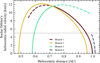 |
Fig. 3 Solar Orbiter’s heliocentric distance and absolute value of its radial velocity. Colors separate individual branches of the orbit that come with changes in orbital parameters at gravity assists. Dashed lines correspond to all the combinations of radial velocity and location, while solid lines denote that Solar Orbiter passed through both inbound and outbound arms for the combination. The horizontal dashed line denotes Solar Orbiter’s radial velocity of 5 km s−1. |
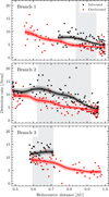 |
Fig. 4 Nonparametric fitting of the detection rate observed between 29 June 2020 and 27 November 2021 in th inbound and outbound part of the trajectory, with branches being separated by gravity assists on 26 December 2020 and 8 August 2021. The lines are the results of non parametric fitting and only grayed intervals are used for further analysis; readers can compare this with Fig. 3. |
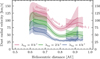 |
Fig. 5 Velocity estimated from TDS/TSWF-E/CNN. Different colors correspond to different assumed background rates. Shaded areas correspond to 50% confidence intervals and the solid lines correspond to median values for a given heliocentric distance. Different branches of λbg = 0 h−1 are labeled. Only parts of the branches where υsc > 5 km s−1 are shown. |
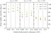 |
Fig. 6 Velocity estimated from TDS/TSWF-E/CNN. Single velocities were obtained from profiles for better readability. The points were con structed as averages of velocities at 0.65,0.75, and 0.85AU for all the branches, where a velocity is the median solution for all the bootstrap replications. For full profiles, readers can refer to Appendix C. |
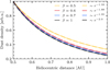 |
Fig. 7 Modeled dust spatial densities for different β values assuming a circular initial orbit of 0.1 AU. Solid lines show the spatial density and they were normalized to the density at 0.5 AU. Dashed lines are approximations to the solid lines, assuming a power dependence on r. |
3.4 Spatial density
If the hyperbolic grains do not accelerate (for example β mete oroids with β ≈ 1 are assumed), a radial dependence of spatial density of ~r−2 is the result. This is not the case if acceleration or deceleration is present. Particularly, it makes sense to assume slowing dust (β < 1), as Fig. 5 suggests slowing rather than accelerating dust. Also, β ≈ 1 or even β > 1 needs a rather specific set of conditions (a combination of material and specific size, see Mann 2010), while 0.5 < β < 1 is possible for a broad range of dust parameters. The observed effective β is then determined by aggregation of all components. The equation for detection rate (4a) contains r–2, but it remains the correct expression for dust flux even if υdust is not constant. In that case, r−2 should not be interpreted as a spatial density of dust, but as a geometric factor. The spatial density is then expressed through the nonconstant υdust. However, this makes it very difficult to fit model (Eq. (4a)) to the data, as υdust is no longer a numeric parameter, but a function of r.
We shall continue to explore the spatial density view and examine the effective exponent of r given β meteoroids with some 0.5 ≤ β < 1. Figure 7 shows an example of how the β value influences the spatial dust density (for a spatial dust density calculation, see Appendix A). The analysis of spatial density as a result of deceleration does not require the dust to be β meteoroids, but the relation to the β value clearly does. In Fig. 7, an initial orbit of 0.1 AU is assumed; readers can refer to Appendix E for plots of the dust spatial density variation similar to Fig. 7 for different initial orbits. The particular exponents depend on the initial orbit, but the general trend of a lower β value implying deceleration remains.
4 Daily count inference
4.1 Model formulation
We decided to model the number of dust detections within a day as a Poisson-distributed random variable, as dust detection itself is a prime example of a Poisson point process in time, as discussed in Sect. 1. The rate λ of the process is considered dependent on multiple parameters θ. Notably, we consider λ to not be explicitly dependent on time, but to be temporarily dependent indirectly, through the orbital parameters and the orbital phase of the spacecraft. Importantly, the rate is also considered dependent on the parameters of the dust cloud. Therefore, we formulated a hierarchical Bayesian model with five parameters, ϵυ, ϵr, λβ, λbg, and vr, which, for simplicity, we denote as θ = (ϵυ, ϵr, λβ, λbg, vr). These parameters were used to model the rate λ and by extension detected counts (see Eqs. (7a) to (7d)). We note that the rate λ (see Eq. (7b)) is a generalization of Eq. (4a) with an additional constant (background) term and a variable exponent of heliocentric distance.
In order to keep the present model simple and yet allow for nonconstant velocity, we used the parameters vr and ϵr as the mean radial dust velocity and density exponent, respectively (see Appendix D for a further interpretation). This combination allows for one to fit a single constant mean velocity and effective acceleration (through the exponent ϵr) at the same time with just two constant scalar parameters. It is important to keep in mind though that the parameter vr is the effective mean radial velocity of the dust grains. The velocity of an individual dust grain changes as it moves through the Solar System. The exact meaning of this effective mean is therefore opaque, as the measurement was done at a variable heliocentric distance. However, the radial velocity between 0.5 AU and 1 AU changes gradually and, in the extreme case of β = 0.5 and r0 = 0.05 AU, it changes by about 30 % (see Fig. 1), which is a smaller difference than the difference due to either different β or r0. Therefore, it is of lesser importance whether the inferred mean is the temporal mean, the spatial mean, or anything in between.
The Poisson likelihood (Eq. (7a)) includes the exposure time E (in hours) and the rate λ (in detections per hour). Then Eq. (7c) is a straightforward definition of relative velocity between the spacecraft and the dust particle, while Eq. (7d) describes the decomposition of dust velocity into radial and azimuthal com ponents. In practice, the model defines the parameter vr as the radial velocity of a dust particle and the variable va as the azimuthal velocity of the same particle, but only vr is regarded as a random variable. The variable va is directly related to heliocentric distance |r| according to Eq. (7e), which is approximately equivalent to the r0 = 0.1 AU line in Fig. 2. This is due to the simpler and less important dependence of υimpact on va and as a compromise in order to keep the number of free parameters reasonable with respect to the available data (the attempts to fit six parameters were not fruitful). The main goal of the fitting procedure is to determine the marginal posterior distributions of each of the parameters θ of the model
 (7a)
(7a)
 (7b)
(7b)
 (7c)
(7c)
 (7d)
(7d)
 (7e)
(7e)
There are N detections observed in a given day, the exposure E is the total time when the instrument was collecting data in a mode that allows for dust detection, hence it is known precisely. The location and velocity of Solar Orbiter are also known precisely. In Eq. (7c), a dimensionless parameter is constructed –it has computational advantages if υimpact ≈ 1, as a rather high power of the variable was computed in the process. Equations (7c)-(7e) explain the role of the parameter υr in Eq. (7b) and they have only been separated from Eq. (7b) for better readability. We note that purely 2D motion of dust particles, within the ecliptic plane, is assumed in Eq. (7d).
The parameter ϵv is the exponent of υimpact in the mean rate formula and it incorporates the dependence on the rate of volume scanning (V/t ∝ S • υimpact), hence  , and the dependence on charge yield a and dust mass power-law exponent δ in the form of υαδ. The dependence is then
  . The parameter ϵr is the exponent of heliocentric distance r, which is notably influenced by acceleration and deceleration of dust, as discussed in Sect. 3.4. Readers can refer to Appendix D for a further interpretation. The parameter λβ plays the role of a normalization constant, accounting for an absolute dust spatial density and spacecraft detection area and holds the physical unit of h−1. It is uninteresting to study this parameter in itself, in the sense that it merely normalizes the model so that the detection rate corresponds to the observed mean rate and has no consequence on the physical characteristics of any given particle. The parameter λbg has the meaning of detections per hour as well, but it is clearly interpreted as the background detection rate, that is to say the rate of detections that are not attributable to hyperbolic dust. The parameter vr also has a very direct meaning, which is the mean outward radial velocity of the hyperbolic dust in our experimental range. We note that variation of impact velocity is still allowed by variation in spacecraft velocity υsc. Acceleration is accounted for in ϵr.
4.2 Prior distributions of parameters
For Bayesian inference, choosing reasonable priors is important. Ideally, priors should be informative (narrow) enough to capture the prior knowledge about parameters, but vague (wide) enough so that they still allow for additional information to play a role. It is physically infeasible for the parameters λβ and λbg to be negative, as they have a meaning of detection rate. Furthermore, positive radial velocity is also required by the model to work. Therefore, we opted for gamma priors for these three parameters. Although we are quite sure about the sign of the parameters ϵv and ϵr, neither the model nor the physical unit actually rules out the possibility of ϵv or ϵr having any sign. We therefore opted for normal priors for ϵv and ϵr. The choice of prior family for ϵv, ϵr, and vr is of little importance. Generally speaking, prior choice makes less of a difference the more data are analyzed.
In order to incorporate our actual prior belief about the model, we chose what we believe are moderately informative priors for the parameters. The following paragraphs discuss our choice. For a graphical representation of the prior distributions of the parameters, readers can refer to Fig. 8.
The parameter ϵv stands for 1 + αδ. Since we have indications from Zaslavsky et al. (2021) that δ ≈ 0.3 and most laboratory experiments show (Collette et al. 2014) that 3 ≲ a ≲ 5, we expect 1.9 ≲ ϵυ = 1 + αδ ≲ 2.5. We therefore chose the prior ϵυ ~ Norm(mean = 2.2, stdev = 0.2), which places emphasis on the range 2.0 < ϵυ < 2.4 and yet does not prohibit any real ϵυ. We note that δ and α are the only pieces of information used for prior construction taken from outside of this work. For more discussion, readers can refer to Appendix I.
Provided that there are no major sources of dust between 0.5 AU and 1 AU and provided that dust neither accelerates nor decelerates, ϵr = –2, which follows easily from mass conservation. If we relax the latter assumption, then ϵr ≠ –2. In fact, the dependence no longer follows  exactly, but as is shown in Fig. 7, for β meteoroids of 0.5 ≲ β ≲ 1 the dependence is very similar to
  with –2 ≲ ϵr ≲ –1.59. We therefore chose a prior ϵr ~ Norm(mean = –1.8, stdeυ = 0.2), which emphasizes the range –2.0 < ϵr < –1.6 but in principle allows for any real ϵr . As for the parameter λβ, we know it is on the order of the total rate, which is 6.9 h−1 on average. The interpretation of the parameter is made less clear by the normalization in Eq. (7c). However, the factor of
  is on the order of 1 and the fac tor of
  is > 1, hence we expect 1 ≲ λβ ≲ 10. We chose a less informative prior of λβ ~ Gamma(shape = 3, scale = 1).
Figure 5 shows that for background detections, λbg < 4 h−1 is feasible. We chose a less informative prior λbg ~ Gamma(shape = 3, scale = 1), which is wide and allows for any positive λbg.
Based on Fig. 6, we believe that values 40 km s−1 ≲ vr ≲ 80 km/s are mostly expected. We chose the prior vr ~ Gamma(shape = 10, scale = 5) that emphasizes that range, with the mean of 50 km s−1, which is the value that Zaslavsky et al. (2021) reported. This prior still allows for any positive value of vr.
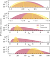 |
Fig. 8 Prior and posterior distributions for the parameters θ. The prior distributions are described in the main text. Summary statistics for posterior distributions are described in Table 1. |
Marginal posterior mean and the standard deviation for all the parameters.
4.3 Posterior distributions
The analysis was performed using TDS/TSWF-E/CNN data. For an analogous analysis performed on Solar Orbiter on board identified dust impacts, readers can refer to Appendix H. Posteriors were inferred using R-INLA. The model (7b) was complicated by the steep dependence of the rate λ, especially the dependence on exponential parameters ϵυ and ϵr. We note that a radial velocity ≳ 60 km/s is consistent with detection rate λbg ≈ 1.5 and αδ ≈ 1.0, according to Fig. 6. It is important to note that the exact choice of priors and other parameters, such as the refer ence azimuthal velocity in Eq. (7c) and the procedure starting point (as INLA works on a grid largely defined by the initial point), influences the exact result; although, no major difference is encountered when parameters or priors are reasonably varied (see Appendix I). As for the initial point, the mode of the joint prior was used: θ = (2.2, –1.8, 2, 2, 45).
Several measures can be used to evaluate the appropriateness of a model to a data set. We inspected the conditional predictive ordinates (CPO) and the predictive integral transform (PIT), which indicated no issues (see Appendix F for details).
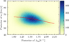 |
Fig. 9 Covariance between vr (radial dust velocity) and λbg (background detection rate); correlation is –0.3. The red line is the mean vr conditioned on λbg and it was produced by sampling from the joint posterior distribution of θ. |
4.4 Discussion of the posterior distribution
The inferred posterior distribution of velocities shown in Fig. 8 is not to be interpreted as a distribution of velocities within the dust cloud directly, but rather as a distribution of the effective mean velocities encountered on each day, or even better - the uncertainty in effective velocity. There could indeed be dust grains with velocity well off the effective support of the posterior distribution, as long as the mean of all velocities does not exceed the region indicated by the posterior distribution.
The θ parameters are not independent. Figure 9 shows the covariance between the vr (radial velocity) and λbg (background detection rate) parameters. A negative correlation suggests that higher vr is likely to occur in the case of lower λbg. This offers a sanity check: a higher velocity would mean a lower difference between an inbound and outbound flux, which has a similar effect to the higher background component scenario - a negative correlation between vr and λbg is thus expected. For covariances between all parameters, readers can refer to Appendix G.
The TDS/TSWF-E/CNN data set contains 6.9 b−1 detections on average. The inferred value of λbg = (1.54 + 0.25) h−1 implies that, in total, (78 + 4) % of dust is attributed to hyperbolic dust within the model. The constant background λbg is the simplest available generalization and is therefore likely an over simplification. The hyperbolic dust detection rate shows a strong negative correlation with heliocentric distance. If, for instance, nonhyperbolic dust shows a similar anticorrelation, the actual nonhyperbolic component is higher than inferred. Conversely, if nonhyperbolic prevalence shows a correlation with the heliocen tric distance, the actual nonhyperbolic component is lower than inferred. Both cases would also imply changes to the inferred parameters of hyperbolic dust (see Appendix J for a visual expla nation). If the nonhyperbolic component is mostly nondust (for example, misattributed electrical phenomena), independence on the heliocentric distance is reasonable. However, if most of the nonhyperbolic contribution is due to bound (Keplerian) dust particles, then anticorrelation is expected. If interstellar dust (ISD) streaming predominantly from one direction approxi mately within the ecliptic plane is present, a positive correlation is also feasible due to the velocity vector orientation.
Indeed, ISD was observed (Baguhl et al. 1996; Zaslavsky et al. 2012; and Malaspina et al. 2014) to arrive mainly from a 258° ecliptic longitude. The highest flux is observed when a spacecraft has an antiparallel velocity, which vaguely coincides with a higher heliocentric distance phase of Solar Orbiter's orbit so far. If ISD is an important contribution to λbg, the actual back ground flux may be lower than the suggested λbg ≈ 1.5 h−1. For now, ISD is not apparent in Solar Orbiter data and the fact that models fit well without ISD suggests it is not an important com ponent of Solar Orbiter detections. Near the solar minimum of 2020, the solar magnetic field had a defocusing configuration with the Lorentz force acting on the interstellar dust in the outer heliosphere pointing away from the heliospheric current sheet (Mann 2010), hence depleting the ISD flux in the near-ecliptic region and inside 1AU. Identifying ISD with Solar Orbiter is, however, beyond the scope of the present work, but it remains worthy of future investigation, especially since ISD may become more important during the current solar cycle (Mann 2010). For now, no bound dust particles are apparent either, nor are the retrograde dust particles. If the constant background is a crude oversimplification and the nonhyperbolic component has a prominent dependence on heliocentric distance, the present interpretation of the θ parameters is not correct, as the model is not on point. Inclusion of more parameters in the model (for example a more sophisticated nonhyperbolic term) may be feasible with more data in the coming months.
The posterior mean of the detection rate is shown in Fig. 10 in units of: m−2h−1, assuming a detection area of 8 m2 (Solar Orbiter thermal shield approximate area); and day−1, taking into account the detection time per day and extrapolating to 24 h. We note that the credible intervals reflect the uncertainty of the inferred mean detection rate (the uncertainty of our knowledge, given the data), which is the same uncertainty as visualized in Fig. 8. The spread of data points in Fig. 10 is much wider and mostly defined by the variance of the Poisson random variable, given the mean rate, rather than the uncertainty in the mean rate. The prediction intervals of the Poisson random variable are shown in Fig. 11 and, there, data points seem to be appropriately covered by the credible intervals.
The inferred value of the parameter ϵr ≈ –1.6 suggests that dust grains are slowing distinctly on their way out of the inner heliosphere between 0.5 AU and 1 AU, resulting in a spatial distribution different from the trivial λ∝ r–2 case. Readers can refer to Fig. 7 for a comparison. With an inferred velocity of (63 + 7) km s−1 between 0.5 AU and 1 AU, significant deceleration suggests a much higher velocity closer to the Sun. Assuming β meteoroids with a circular initial orbit, the ϵr value implies a specific β value needed for just the right level of deceleration. Deceleration is a result of energy transfer from kinetic to potential, and therefore, given the initial heliocentric distance, the deceleration rate depends on the initial velocity. This makes the assumption of a circular initial orbit crucial when we are to infer the β parameter. For example, a β value needed to explain an observed ϵr is different if the β meteoroid parent object has an eccentricity of 0.3, rather than 0. For an analysis of the implied β values in the case of the circular parent orbit, readers can refer to Fig. 12. Various initial parent body orbit radii are shown in Fig. 12 to demonstrate that the model is not very sensitive to that parameter. For comparison, we note that velocities ≳ 60 km s−1 are consistent with β ≈ 0.6 and the origin between 0.05 AU and 0.1 AU, according to Fig. 1. We note that 0.05 AU ≈ 10 R⊙, where R⊙ is the Solar radius.
However, it is feasible to expect a parent body with an eccen tricity of 0.3, as the mean eccentricity in the inner asteroid belt is e ≈ 0.15 (Malhotra & Wang 2016). If a dust grain is ejected from a given heliocentric distance r, the eccentricity e = 0.3 implies a +14% ejection speed if r is the perihelion and a -16% ejection speed if r is the aphelion, compared to ejection from a circular orbit of radius r. In the case of e ≠ 0, β > 0.5 is not the right condition for the unbound β meteoroid. In fact, for e = 0.3 the condition is approximately β > 0.35 for peri helion, and β > 0.65 for aphelion ejection. It is important to keep in mind that the +14% could also be ∆υ transferred at colli sion, as collisions between larger dust objects are likely a major source of meteoroids. Then the 14% relative speed would, for instance, correspond to the collision of two asteroids on circular orbits with a relative inclination of 8°, which is also a very feasible scenario. For instance, if the example of +14% of ∆υ (or an eccentricity of 0.3) is a good representative of the process, the resulting implied β would be not β ≳ 0.5, but rather β ≳ 0.35. Eccentricities and relative velocities in the zodiacal cloud remain uncertain. We note that even in the described case, we are still considering a dust grain with a purely azimuthal velocity at liberation, which is yet another simplification.
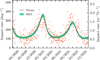 |
Fig. 10 Estimated posterior mean of the dust impact with 90 % HPD credible intervals. The credible intervals are not supposed to cover the data scatter (see text for an interpretation of the credible intervals that are shown). |
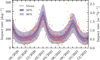 |
Fig. 11 Estimated posterior mean of the hyperbolic dust detections and HPD prediction intervals. The prediction intervals are supposed to cover the data scatter (see text for an interpretation of the prediction intervals that are shown). |
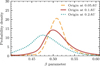 |
Fig. 12 β parameter resulting from ϵυ posterior distribution under the assumption of a circular parent body orbit (see text for a discussion). |
4.5 Comparison with previous results
As Solar Orbiter has been operated only since 2020 and will be operated at least until 2027, the results presented in this paper are one of the earlier ones for the mission. Based on similar data, though collected over a shorter time period, Zaslavsky et al. (2021) have reported several physical parameters of the β-meteoroid population. Interestingly, they have reported radial velocity to be about 50 km s−1, which is within two standard deviations from (63 ± 7) km s−1 reported here, but it is important to bear in mind that the number was inferred under substantially different assumptions. The velocity is crucial to infer the β-meteoroid flux at 1 AU for example, which Zaslavsky et al. (2021) have reported to be 8 × 10⁻⁵ m−2s−1. Under our model assumptions (constant radial dust velocity) and taking the joint posterior distribution of the parameters, we report (1.6 ± 0.1) × 10−4 m−2s−1 for hyperbolic dust and the residual component (λbg) together (measured on a stationary spherical object, per m2 of the cross section), a value higher by a factor of ≈2. For the component consistent with hyperbolic dust only, we report the flux of (1.1 ± 0.2) × 10−4 m−2s−1 and for the component attributed to the residual, background component (5.4 ± 1.5) × 10−5 m−2s−1. As for αδ (keeping in mind that αδ = ϵυ –1 here), Zaslavsky et al. (2021) have reported consistency with αδ = 1.3, while we report ϵυ –1 = (1.04 ± 0.20).
As for a comparison of the present results with the β-meteoroid flux near 1 AU, Wehry & Mann (1999) reported the flux of β meteoroids in the ecliptic plane detected by Ulysses between 1.0–1.6AU to be (1.5 ± 0.3) × 10−4 m−2s−1. Zaslavsky et al. (2012) reported a flux of β meteoroids at 1 AU of size 100–300nm on STEREO/Waves in the range of 1-6 × 10⁻⁵ m−2s−1, which is a somewhat lower value than reported here. Solar Orbiter detections are likely of 100 nm and larger dust, but the upper limit is somewhat higher for Solar Orbiter due to a wider dynamic range (3–150 mV for STEREO and 3–700 mV for Solar Orbiter), which may account for some of the difference. Malaspina et al. (2015), however, reported the value for STEREO/Waves by about a factor of 2.5 higher than Zaslavsky et al. (2012), which is on its upper bound virtually identical to the value reported here. For the Wind/WAVES experiment, Malaspina et al. (2014) reported (2.7 ± 1.4) × 10−5 m−2s−1 for the sum of β meteoroids and interstellar dust of 0.1–11 μm size. It has yet to be determined if and how much interstellar dust contributes to the measurements of Solar Orbiter's RPW analyzed in the present work. Recently, Szalay et al. (2021) have reported 4–8 × 10⁻⁵ m−2s−1 for the β-meteoroid flux at 1 AU measured with Parker Solar Probe. The upper bound of this estimate is similar to the value reported in the present work.
5 Conclusions
We have presented the analysis of the velocity of hyperbolic dust grains between 0.5 AU and 1 AU based on the highest-quality available data on daily dust detections by Solar Orbiter's RPW, including a discussion of implications for the velocity in the case of nonhyperbolic (be it another dust population or false detections) component to the counts. Velocities in the range 30 110 km s−1 are compatible with the data. We have presented a Bayesian hierarchical model and demonstrated how it is used to infer physical parameters of the hyperbolic dust population in the studied region. It is likely that (1.5 ± 0.3) h−1 are in fact not caused by hyperbolic dust. Then observations are consistent with a mean radial velocity of the hyperbolic component (63 ± 7) km s−1 between 0.5 AU and 1 AU. Spatial dependence of the detection rate suggests substantial deceleration of the observed hyperbolic dust particles. If they are imeteoroids, the value of β is likely just above the liberation threshold, specifically β ≳ 0.5 under the assumption of circular orbits of parent bodies. Hence closer to their origin, they likely have velocities higher than the inferred (63 ± 7) km s−1. As a result of our modeling, we provide estimates of hyperbolic dust flux at 1 AU of (1.1 ± 0.2) × 10−4 m−2s−1, which is a value compatible with the results of other relevant measurements.
6 Outlook
Solar Orbiter will be significantly inclined, starting in 2025, which will require further generalization of the model to account for the dust distribution out of the ecliptic plane. The parameters of hyperbolic dust out of ecliptic will likely provide more information on in-ecliptic hyperbolic dust, such as its parent bodies'mean eccentricity. Due to independence on β, knowledge of the azimuthal velocity would be a good indicator of the origin of β meteoroids, but it is hard to infer as the azimuthal component is much smaller than the radial component. The ecliptic detections may help in this regard as well.
As mentioned earlier, the de-focusing solar magnetic field configuration near the 2020 solar minimum does not favor the detection of ISD. With solar cycle 25, the focusing field configuration will return at some time before the solar minimum of 2031. It is possible that a significant ISD component will be observed in the years following the solar maximum of 2025, which will, if observed, provide new opportunities for dust population discrimination and a more comprehensive dust cloud description thanks to Solar Orbiter RPW data.
Acknowledgements
Author contributions: Concept: S.K., A.T., I.M. Data analysis: S.K., S.H.S., A.K. Interpretation: S.K., I.M., A.T., S.H.S., A.K., A.Z. Manuscript preparation: S.K. The code and the data used in present work are publicly available at https://github.com/SamuelKo1687/solo_dust_2822. This work made use of publicly available data provided by A. Kvammen: https://github.com/AndreasKvammen/ML_dust_detection. S.K. and A.T. are supported by the Tromsø Research Foundation under the grant 19-SG-AT. This work on dust observations in the inner heliosphere is supported by the Research Council of Norway ( grant number 262941). In addition, A.K.acknowledges the support from the Research Council of Norway (grant number 326039). Authors sincerely appreciate the support of Solar Orbiter/RPW Investigation team and thank the anonymous reviewer for constructive comments. This work was made possible by R-INLA package, authors thank to R-INLA team, see https://www.r-inla.org.
Appendix A Single-particle velocity and spatial density
For the purposes of Figs. 2 and 1 , dust grains were assumed to move within the ecliptics, liberated from an initially circular orbit and with their motion governed by the gravity and solar radiation pressure only; therefore,
 (A.1)
(A.1)
 (A.2)
(A.2)
 (A.3)
(A.3)
where υ0 is the initial (purely radial) velocity and r0 is the initial heliocentric distance (radius of the circular orbit). Furthermore, given a radial velocity profile of a radially escaping dust grain υrad (r), the dust spatial density ρ at a heliocentric distance r is
 (A.4)
(A.4)
where r0 is a reference heliocentric distance.
Appendix B Dust radial velocity estimation
If we suppose that the detection rate is proportional to  then
then
 (B.1)
(B.1)
![Mathematical equation: $ = {R_0}{\left[ {\sqrt {{{\left( {{\upsilon _{dust;rad}} - {\upsilon _{sc;rad}}} \right)}^2} + \upsilon _{sc;azim}^2} } \right]^q}, $](/articles/aa/full_html/2023/02/aa45165-22/aa45165-22-eq28.png) (B.2)
(B.2)
where we assumed υdust;azim = 0. Then, at any given heliocentric distance r,
 (B.3)
(B.3)
 (B.4)
(B.4)
and therefore
 (B.5)
(B.5)
from which
 (B.6)
(B.6)
 (B.7)
(B.7)
 (B.8)
(B.8)
which leads to a quadratic root of
 (B.9)
(B.9)
 (B.10)
where (+) in Eq. (B.9) leads to positive velocity υsc;rad. It is easy to see that in the special case of q = 1; υsc;azim = 0 that
![Mathematical equation: $ D = 4\upsilon _{sc;rad}^2\left[ {{{\left( {R_{in}^2 + R_{out}^2} \right)}^2} - {{\left( {R_{in}^2 - R_{out}^2} \right)}^2}} \right], $](/articles/aa/full_html/2023/02/aa45165-22/aa45165-22-eq37.png) (B.11)
(B.11)
 (B.12)
and, by extension,
![Mathematical equation: $ {\upsilon _{dust;rad}} = {{\left| {{\upsilon _{sc;rad}}} \right|\left[ {\left( {R_{in}^2 + R_{out}^2} \right) \pm 2{R_{in}}{R_{out}}} \right]} \over {\left( {R_{in}^2 - R_{out}^2} \right)}}, $](/articles/aa/full_html/2023/02/aa45165-22/aa45165-22-eq39.png) (B.13)
(B.13)
which is
 (B.14)
for (+) in the numerator.
Appendix C Velocity inference — Full velocity profiles
The velocity profiles inferred in Section 3.2 are shown in Figs. C.l to C.3 (readers can compare them to Figs. 5 and 6). We note that the missing solutions (jittery line) for heliocentric distance > 0.7 AU and λbg = 4 cause incomplete data shown in Fig. 6. These solutions only exist for some combinations of the free parameters, in particular for λbg = 4.
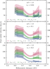 |
Fig. C.1 Velocity estimated from TDS/TSWF-E/CNN under the assumption of αδ = 1.0. The panels correspond to different initial heliocentric distances. The colors correspond to different assumptions as to the background detection rate. |
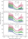 |
Fig. C.2 Velocity estimated from TDS/TSWF-E/CNN under the assumption of αδ = 1.3. The panels correspond to different initial heliocentric distances. The colors correspond to different assumptions as to the background detection rate. |
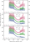 |
Fig. C.3 Velocity estimated from TDS/TSWF-E/CNN under the assumption of αδ = 1.6. The panels correspond to different initial heliocentric distances. The colors correspond to different assumptions as to the background detection rate. |
Appendix D Interpretation of the parameter ϵr
An intuitive explanation of the parameter vr as the mean dust velocity and of the factor  as the spatial density can be clarified, assuming vr ∝ rξ. With the model (7b), the nonconstant component
  of the rate R is proportional to
 (D.1)
(D.1)
where ϵr = –2 in the case of no acceleration of the dust. Furthermore, ϵυ is explained as ϵυ = 1 + αδ, and therefore
 (D.2)
(D.2)
The factor of  actually comes from the proportionality
 (D.3)
(D.3)
if we assume only radial motion for simplicity; readers can compare this with Eq. (4a). It is also apparent from the following: Assuming a stationary spacecraft (υimpact = vr), the detection rate (in s−1) is a product of the flux F(r) (in s−1) and the detection area S (in m2), independently of vr. We therefore have, for nonaccelerating dust,
 (D.4)
(D.4)
and finally assuming vr ∝ rξ, we get
 (D.5)
(D.5)
and therefore
 (D.6)
(D.6)
There is a dichotomy in Eq. (D.5) in that the assumption of vdust ∝ rξ was used to expand the υdust but not the υimpact. This is one way of interpreting the approximation described in Section 4.1; we assumed a nonconstant dust velocity in the factor for the spatial dust density, but a constant radial dust velocity in the expression for υimpact (see Eq. (7c)). This was done because of a clear relation of  to acceleration and deceleration of the dust, which in our case (ϵr ≈ –1.6 => ξ ≈ –0.4) reveals that the dust is decidedly decelerating.
Appendix E Spatial density profiles
We assumed that the initial orbital distance influences the relationship between β values and the spatial dust density profiles. In Fig. 7, the initial orbit of 0.1 AU was assumed. Readers can refer to plots E.l and E.2 for similar plots with different assumptions as to the initial orbit., and Fig. E.3 for a similar plot if the eccentricity of e = 0.2 and the perihelion ejection with a perihelion of r = 0.1 AU is assumed. Although the estimates of the exponents vary, the general conclusion of a lower β implying a lower exponent holds. We note that the profile gets significantly influenced when β is close to the threshold, and that it depends on the initial orbit and eccentricity. Therefore, β < 0.5 is shown where 0.5 is much higher than the liberation threshold.
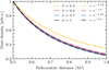 |
Fig. E.1 Modeled dust spatial densities for different β values assuming a circular initial orbit of 0.05 AU. The solid lines show the spatial density and are normalized to the density at 0.5 AU. The dashed lines are approximations to the solid lines, assuming a power dependence on r. |
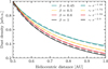 |
Fig. E.2 Modeled dust spatial densities for different β values assuming a circular initial orbit of 0.2 AU. The solid lines show the spatial density and are normalized to the density at 0.5 AU. The dashed lines are approximations to the solid lines, assuming a power dependence on r. |
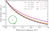 |
Fig. E.3 Modeled dust spatial densities for different β values assuming an elliptical initial orbit with an eccentricity of e = 0.2 and perihelion ejection. A perihelion of 0.1 AU was assumed. The solid lines show the spatial density and are normalized to the density at 0.5 AU. The dashed lines are approximations to the solid lines, assuming a power dependence on r. |
Appendix F Model assessment
There are several options for model evaluation implemented in R-INLA (Gómez-Rubio 2020, Chapter 2.4). We briefly describe two measures of choice.
The conditional predictive ordinates (CPO, see Pettit (1990)) for a given observation point gives the posterior probability of each observation when this observation is omitted in the model fitting. CPO is used to detect surprising observations or outliers. We examined the fit for failure flags for all the points, which would suggest a contradiction between the model and a data point. No failures were encountered.
The predictive integral transform (PIT, see Marshall & Spiegelhalter (2003)) measures the probability that a new observation will be lower than the observed value for each observation point individually. The histogram of the PIT values should therefore be similar to the uniform distribution between 0 and 1 when the model explains the data well (see Fig. F.1).
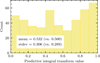 |
Fig. F.1 Histogram of PIT values for the model described in Section 4.3. Mean and standard deviation were compared to the values for uniform distribution. |
Appendix G Covariance plots of posteriors
As is shown in figure G.1, basically all parameter pairs show a substantial correlation. The pairs hold useful information, but this is hardly surprising and they are easy to interpret, with the Eq. (7b) model in mind. The correlation is unimportant in the case of λβ, which has a role of a normalization constant.
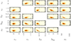 |
Fig. G.1 Illustration of the covariance between all parameter pairs, constructed using sampling from the joint posterior distribution of all parameters. |
Covariance between all parameter pairs, constructed using sampling from the joint posterior distribution of all parameters.
Appendix H Model fitting to original data
The procedure described in sec. 4 was also applied to the original TDS data, meaning impacts were identified onboard Solar Orbiter, described by Maksimovic et al. (2020), which are different from TDS/TSWF-E/CNN data (Kvammen et al. 2023) used otherwise in sec. 4. The CNN-refined data used in sec. 4 have fewer type 1 and type 2 errors, as well as better correspondence with visual inspection by experts than the original data (see discussion in Kvammen et al. (2023)). However, the original data were used previously (Zaslavsky et al. 2021) and the inspection of the result of the procedure is instructive nonetheless. The results are presented in Fig. H.1.
The most important and intuitive difference is that a much lower λbg is inferred in this case (readers can compare this with Fig. 8). As described in Kvammen et al. (2023), the CNN procedure identifies substantially more impacts near-aphelion, which suggests more background dust, with everything else being equal. It is important to keep in mind that, as evaluated by Kvammen et al., the prevalence of impacts erroneously labeled as dust impacts among TDS data is close to 20 %, which is much higher than λbg infered here.
Importantly, the inferred velocity vr does not change substantially, even though ϵυ and especially ϵr do change consequentially. Importantly,ϵr < –2 implies accelerating dust, which implies β> 1 and requires specific material and a particular size of the grains, hence this is unlikely — at least for β meteoroids. We note that ϵr is effectively far from our prior expectations, providing a poor fit to our prior knowledge. These results lend additional credence to the improvement of the CNN data.
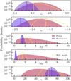 |
Fig. H.1 Prior and posterior distributions of parameters, making use of the original TDS (onboard processed) data. Prior distributions are described in the main text in sec. 4. Posterior distributions are described in Tab. H.1. Posteriors from Fig. 8 are shown as a reference in dashed lines for comparison. |
Appendix I Variation of priors and model parameters
In this appendix, we investigate the dependence of the results in sec. 4 on the model parameters and priors. To contextualize this variation, we review how the priors and model parameters depend on previous work, in particular Zaslavsky et al. (2021).
The velocity vr has been inferred independently in this work and the fact that it is found to be compatible with the findings of Zaslavsky et al. is only reassuring. The velocity va was assumed based on first principles (see Section 4.1) and is of lesser importance compared to vr. The background detection rare Abg is discussed in the present work, independent of any previous findings and the rate λβ merely serves the role of a normalization constant. Both rates are closely tied to the observed counts and are therefore constrained by the data. The exponent ∈r is discussed and assessed from first principles in the present work, while the exponent ϵv is inspired by Zaslavsky et al. (2021). The designated prior mean of 2.2 decomposes to the sum of 1 (from first principles) and 1.2 = αδ, where only δ ≈ 0.34 ± 0.07 is taken from Zaslavsky et al. (2021) and where the uncertainty of 0.07 corresponds to a 95% confidence. Moreover, δ there is not yielded by Zaslavsky et al. from the fit to the flux, but rather from the analysis of the charge distribution presented therein, which adds another piece of information, independent from the flux itself. For simplicity, we used the value of Zaslavsky et al. for δ and the same analysis of TDS/TSWF-E/CNN data yields very similar results. Then a is known from laboratory measurements, for example from McBride & McDonnell (1999) and Collette et al. (2014). Collette et al. found α ≈ 4 for most materials. For consistency, however, we continued to use the findings of McBride & McDonnell, who reported α ≈ 3.5. Assuming 95 % confidence of α ≈ 3.5 ± 1, we arrived at αδ ≈ 1.2 ± 0.4 in terms of 95 % confidence. We therefore believe that the standard deviation of the ev prior of 0.2 represents the uncertainty well. Further analysis shows that ϵυ is not inferred substantially differently in the case of wider priors for the parameters (see Fig. I.1 for an example). The figure shows that in the case in which all parameter priors are considered to be broader, the result mean stays within the reference posterior credible range. Also a practically flat prior for ϵυ leads to a similar posterior, given the remaining priors are taken as in Fig. 8.
It is true that the priors themselves express the uncertainty in prior knowledge; however, to demonstrate the robustness of the analysis, we here show perturbed priors and the resulting posterior combinations (Figs. I.1 and I.2) to show that the result -though somewhat dependent on the prior selection - does not change dramatically if priors are chosen arbitrarily slightly differently. Also the choice of the value of parameter va (which is not a free parameter in our modeling, see Eq. (7e)) is examined here (see Figs. I.3 and I.4). Last but not least, we show the posteriors in the case of change of the initialization of the iterative procedure to estimate the parameters (Fig. I.5). We do not claim that any of these results is as trustworthy as the main result shown in Fig. 8; we had reasoning behind choosing the priors and parameters that we chose. We note that the mean of the marginal posteriors shown in Figs. I.1 to I.5 lie within high credibility regions of posteriors shown in Fig. 8 and vice versa, which supports the claim that the analysis presented here is robust. It is important to observe that parameter values inferred with a lower precision (wider posterior distributions) are more susceptible to change due to a change in parameters, which is in line with expectations and with the meaning of precision here. A good choice of priors is still important to get the highest quality estimate, but the result is not critically sensitive.
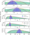 |
Fig. I.1 Prior and posterior distributions of the parameters, with the priors being substantially wider (less informative). The priors and posteriors from Fig. 8 are shown with dashed lines for comparison. |
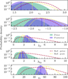 |
Fig. I.2 Prior and posterior distributions of parameters, with priors shifted toward lower values. The priors and posteriors from Fig. 8 are shown with dashed lines for comparison. |
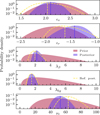 |
Fig. I.3 Prior and posterior distributions of parameters, with the fixed parameter of azimuthal velocity having been changed from 12 km/s at 0.75 AU to constant Okm/s. The posteriors from Fig. 8 are shown with dashed lines for comparison. |
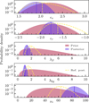 |
Fig. I.4 Prior and posterior distributions of parameters, with the fixed parameter of azimuthal velocity at 0.75 AU having been changed from 12 km/s to 24 km/s, which is a value higher by 100 %. The posteriors from Fig. 8 are shown with dashed lines for comparison. |
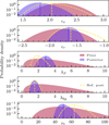 |
Fig. I.5 Prior and posterior distributions of parameters, with a starting point of ϵυ = 3;ϵr = –3;λβ = 3;λbg = 3; vr = 30. The posteriors from Fig. 8 are shown with dashed lines for comparison. |
Appendix J Possible background profiles
In the present analysis, the nonhyperbolic component was assumed to be present and constant. Readers can refer to Fig. J.1 for examples of possible nonhyperbolic component profiles, as discussed in Section 4.4. In the plot, the mean rate of the nonhyperbolic component is the same in all three panels. We note that despite that, the dynamic range (that is ratios of maximum over minimum values) changes significantly as a result of the change in the temporal profile of the nonhyperbolic component. A significant deviation from the constant case would therefore likely change both the inferred prevalence of the nonhyperbolic component and the parameters of the hyperbolic grains.
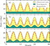 |
Fig. J.1 Detection rate: selection of different combinations of hyperbolic and nonhyperbolic rates compounding to the same observed detection rate. In panel a), the background component is independent of the heliocentric distance. In panel b), the nonhyperbolic component is negatively correlated with the heliocentric distance. In panel c), the nonhyperbolic component is positively correlated with the heliocentric distance. |
References
- Alexander, W., & Bohn, J. 1968, in COSPAR Plenary Meeting, No. NSSDC-ID-66-049A-21-PM (North-Holland Publishing Co.) [Google Scholar]
- Baguhl, M., Grün, E., & Landgraf, M. 1996, Space Sci. Rev., 78, 165 [Google Scholar]
- Collette, A., Grün, E., Malaspina, D., & Sternovsky, Z. 2014, J. Geophys. Res.: Space Phys., 119, 6019 [NASA ADS] [CrossRef] [Google Scholar]
- Czechowski, A., & Mann, I. 2021, A&A, 652, A131 [NASA ADS] [CrossRef] [EDP Sciences] [Google Scholar]
- Dietzel, H., Neukum, G., & Rauser, P. 1972, J. Geophys. Res., 77, 1375 [NASA ADS] [CrossRef] [Google Scholar]
- Dietzel, H., Eichhorn, G., Fechtig, H., et al. 1973, J. Phys. E: Sci. Instrum., 6, 209 [NASA ADS] [CrossRef] [Google Scholar]
- Dohnanyi, J. 1970, J. Geophys. Res., 75, 3468 [NASA ADS] [CrossRef] [Google Scholar]
- Dohnanyi, J. 1972, Icarus, 17, 1 [NASA ADS] [CrossRef] [Google Scholar]
- Friichtenicht, J. 1962, Rev. Sci. Instrum., 33, 209 [NASA ADS] [CrossRef] [Google Scholar]
- Gasque, C., Bale, S., Bowen, T., et al. 2022, AGU Fall Meeting 2021 [Google Scholar]
- Gómez-Rubio, V. 2020, Bayesian Inference with INLA (CRC Press) [CrossRef] [Google Scholar]
- Grün, E. 1984, in The Giotto Spacecraft Impact-induced Plasma Environment (ESA SP), 224, 39 [Google Scholar]
- Grün, E., Zook, H. A., Fechtig, H., & Giese, R. 1985, Icarus, 62, 244 [NASA ADS] [CrossRef] [Google Scholar]
- Grün, E., Pawlinka, S., & Srama, R. 2007, Dust accelerator tests with Cassini RPWS samples (Max-Planck-Institut für Kernphysik), Tech. Rep. [Google Scholar]
- Gurnett, D., Ansher, J., Kurth, W., & Granroth, L. 1997, Geophys. Res. Lett., 24, 3125 [NASA ADS] [CrossRef] [Google Scholar]
- Howard, R. A., Vourlidas, A., Bothmer, V., et al. 2019, Nature, 576, 232 [Google Scholar]
- Kurth, W., Averkamp, T., Gurnett, D., & Wang, Z. 2006, Planet. Space Sci., 54, 988 [NASA ADS] [CrossRef] [Google Scholar]
- Kvammen, A., Wickstrøm, K., Kociscak, S., et al. 2023, Ann. Geophys., 41, 69 [NASA ADS] [CrossRef] [Google Scholar]
- Leinert, C., Richter, I., Pitz, E., & Planck, B. 1981, A&A, 103, 177 [NASA ADS] [Google Scholar]
- Maksimovic, M., Bale, S., Chust, T., et al. 2020, A&A, 642, A12 [NASA ADS] [CrossRef] [EDP Sciences] [Google Scholar]
- Malaspina, D., Horányi, M., Zaslavsky, A., et al. 2014, Geophys. Res. Lett., 41, 266 [NASA ADS] [CrossRef] [Google Scholar]
- Malaspina, D. M., O’Brien, L. E., Thayer, F., Sternovsky, Z., & Collette, A. 2015, J. Geophys. Res.: Space Phys., 120, 6085 [NASA ADS] [CrossRef] [Google Scholar]
- Malaspina, D. M., Szalay, J. R., Pokornỳ, P., et al. 2020, ApJ, 892, 115 [NASA ADS] [CrossRef] [Google Scholar]
- Malaspina, D. M., Stenborg, G., Mehoke, D., et al. 2022, ApJ, 925, 27 [NASA ADS] [CrossRef] [Google Scholar]
- Malhotra, R., & Wang, X. 2016, MNRAS, 465, 4381 [Google Scholar]
- Mann, I. 2010, Annu. Rev. Astron. Astrophys., 48, 173 [CrossRef] [Google Scholar]
- Mann, I., & Czechowski, A. 2005, ApJ, 621, L73 [NASA ADS] [CrossRef] [Google Scholar]
- Mann, I., & Czechowski, A. 2021, A&A, 650, A29 [NASA ADS] [CrossRef] [EDP Sciences] [Google Scholar]
- Mann, I., Meyer-Vernet, N., & Czechowski, A. 2014, Phys. Rep., 536, 1 [Google Scholar]
- Mann, I., Nouzak, L., Vaverka, J., et al. 2019, Ann. Geophys., 37, 1121 [Google Scholar]
- Marshall, E., & Spiegelhalter, D. 2003, Stat. Med., 22, 1649 [CrossRef] [Google Scholar]
- Martins, T. G., Simpson, D., Lindgren, F., & Rue, H. 2013, Comput. Stat. Data Anal., 67, 68 [CrossRef] [Google Scholar]
- McBride, N., & McDonnell, J. 1999, Planet. Space Sci., 47, 1005 [CrossRef] [Google Scholar]
- Meyer-Vernet, N., Aubier, M., & Pedersen, B. 1986, Geophys. Res. Lett., 13, 617 [NASA ADS] [CrossRef] [Google Scholar]
- Meyer-Vernet, N., Moncuquet, M., Issautier, K., & Schippers, P. 2017, J. Geophys. Res.: Space Phys., 122, 8 [NASA ADS] [CrossRef] [Google Scholar]
- Mozer, F., Agapitov, O., Bale, S., et al. 2020, ApJS, 246, 50 [NASA ADS] [CrossRef] [Google Scholar]
- Nadaraya, E. A. 1964, Theory Probab. Applic., 9, 141 [CrossRef] [Google Scholar]
- Nouzk, L., James, D., Nemecek, Z., et al. 2021, ApJ, 909, 132 [NASA ADS] [CrossRef] [Google Scholar]
- Pettit, L. 1990, J. Roy. Stat. Soc. B (Stat. Methodol.), 52, 175 [Google Scholar]
- Rackovic Babic, K., Zaslavsky, A., Issautier, K., Meyer-Vernet, N., & Onic, D. 2022, A&A, 659, A15 [NASA ADS] [CrossRef] [EDP Sciences] [Google Scholar]
- Ragot, B., & Kahler, S. 2003, ApJ, 594, 1049 [NASA ADS] [CrossRef] [Google Scholar]
- Rue, H., Martino, S., & Chopin, N. 2009, J. Roy. Stat. Soc. B (Stat. Methodol.), 71, 319 [CrossRef] [Google Scholar]
- Rue, H., Riebler, A., Sørbye, S. H., et al. 2017, Annu. Rev. Stat. Applic., 4, 395 [NASA ADS] [CrossRef] [Google Scholar]
- Shen, M. M., Sternovsky, Z., Garzelli, A., & Malaspina, D. M. 2021, J. Geophys. Res.: Space Phys., 126, e2021JA029645 [Google Scholar]
- Shu, A., Collette, A., Drake, K., et al. 2012, Rev. Sci. Instrum., 83, 075108 [CrossRef] [Google Scholar]
- Srama, R., Ahrens, T. J., Altobelli, N., et al. 2004, in The Cassini-Huygens Mission (Springer), ed. C. T. Russell, 465 [CrossRef] [Google Scholar]
- Stenborg, G., Howard, R., Hess, P., & Gallagher, B. 2021, A&A, 650, A28 [NASA ADS] [CrossRef] [EDP Sciences] [Google Scholar]
- Szalay, J., Pokornỳ, P., Malaspina, D., et al. 2021, Planet. Sci. J., 2, 185 [NASA ADS] [CrossRef] [Google Scholar]
- Van de Hulst, H. 1947, ApJ, 105 [Google Scholar]
- Vaverka, J., Pellinen-Wannberg, A., Kero, J., et al. 2017, IEEE Trans. Plasma Sci., 45, 2048 [CrossRef] [Google Scholar]
- Vaverka, J., Nakamura, T., Kero, J., et al. 2018, J. Geophys. Res.: Space Phys., 123, 6119 [NASA ADS] [CrossRef] [Google Scholar]
- Wang, Z., Gurnett, D., Averkamp, T., Persoon, A., & Kurth, W. 2006, Planet. Space Sci., 54, 957 [NASA ADS] [CrossRef] [Google Scholar]
- Watson, G. S. 1964, Sankhyā: Indian J. Stat. A, 359 [Google Scholar]
- Wehry, A., & Mann, I. 1999, A&A, 341, 296 [NASA ADS] [Google Scholar]
- Whipple, F. L. 1967, The Zodiacal Light and the Interplanetary Medium (National Aeronautics and Space Administration), ed. J. L. Weinberg, 409 [Google Scholar]
- Zaslavsky, A. 2015, J. Geophys. Res.: Space Phys., 120, 855 [NASA ADS] [CrossRef] [Google Scholar]
- Zaslavsky, A., Meyer-Vernet, N., Mann, I., et al. 2012, J. Geophys. Res.: Space Phys., 117 [Google Scholar]
- Zaslavsky, A., Mann, I., Soucek, J., et al. 2021, A&A, 656, A30 [NASA ADS] [CrossRef] [EDP Sciences] [Google Scholar]
- Zook, H. A., & Berg, O. E. 1975, Planet. Space Sci., 23, 183 [Google Scholar]
Solar Orbiter / Radio and Plasma Waves Data, data retrieved from Observatoire de Paris, LESIA, https://rpw.lesia.obspm.fr/roc/data/pub/solo/rpw/data/L2/
All Tables
Covariance between all parameter pairs, constructed using sampling from the joint posterior distribution of all parameters.
All Figures
|
Fig. 1 Radial velocity profiles of β meteoroids released by a sudden parameter change (for example due to a collision) from an initially cir cular orbit. A selection of β values and origins (r0) is shown. |
| In the text | |
|
Fig. 2 Azimuthal velocity profiles of β meteoroids released by a sudden parameter change (for example, due to a collision) from an initially circular orbit. A selection of origins (r0) is shown, with the β value not being relevant. |
| In the text | |
|
Fig. 3 Solar Orbiter’s heliocentric distance and absolute value of its radial velocity. Colors separate individual branches of the orbit that come with changes in orbital parameters at gravity assists. Dashed lines correspond to all the combinations of radial velocity and location, while solid lines denote that Solar Orbiter passed through both inbound and outbound arms for the combination. The horizontal dashed line denotes Solar Orbiter’s radial velocity of 5 km s−1. |
| In the text | |
|
Fig. 4 Nonparametric fitting of the detection rate observed between 29 June 2020 and 27 November 2021 in th inbound and outbound part of the trajectory, with branches being separated by gravity assists on 26 December 2020 and 8 August 2021. The lines are the results of non parametric fitting and only grayed intervals are used for further analysis; readers can compare this with Fig. 3. |
| In the text | |
|
Fig. 5 Velocity estimated from TDS/TSWF-E/CNN. Different colors correspond to different assumed background rates. Shaded areas correspond to 50% confidence intervals and the solid lines correspond to median values for a given heliocentric distance. Different branches of λbg = 0 h−1 are labeled. Only parts of the branches where υsc > 5 km s−1 are shown. |
| In the text | |
|
Fig. 6 Velocity estimated from TDS/TSWF-E/CNN. Single velocities were obtained from profiles for better readability. The points were con structed as averages of velocities at 0.65,0.75, and 0.85AU for all the branches, where a velocity is the median solution for all the bootstrap replications. For full profiles, readers can refer to Appendix C. |
| In the text | |
|
Fig. 7 Modeled dust spatial densities for different β values assuming a circular initial orbit of 0.1 AU. Solid lines show the spatial density and they were normalized to the density at 0.5 AU. Dashed lines are approximations to the solid lines, assuming a power dependence on r. |
| In the text | |
|
Fig. 8 Prior and posterior distributions for the parameters θ. The prior distributions are described in the main text. Summary statistics for posterior distributions are described in Table 1. |
| In the text | |
|
Fig. 9 Covariance between vr (radial dust velocity) and λbg (background detection rate); correlation is –0.3. The red line is the mean vr conditioned on λbg and it was produced by sampling from the joint posterior distribution of θ. |
| In the text | |
|
Fig. 10 Estimated posterior mean of the dust impact with 90 % HPD credible intervals. The credible intervals are not supposed to cover the data scatter (see text for an interpretation of the credible intervals that are shown). |
| In the text | |
|
Fig. 11 Estimated posterior mean of the hyperbolic dust detections and HPD prediction intervals. The prediction intervals are supposed to cover the data scatter (see text for an interpretation of the prediction intervals that are shown). |
| In the text | |
|
Fig. 12 β parameter resulting from ϵυ posterior distribution under the assumption of a circular parent body orbit (see text for a discussion). |
| In the text | |
|
Fig. C.1 Velocity estimated from TDS/TSWF-E/CNN under the assumption of αδ = 1.0. The panels correspond to different initial heliocentric distances. The colors correspond to different assumptions as to the background detection rate. |
| In the text | |
|
Fig. C.2 Velocity estimated from TDS/TSWF-E/CNN under the assumption of αδ = 1.3. The panels correspond to different initial heliocentric distances. The colors correspond to different assumptions as to the background detection rate. |
| In the text | |
|
Fig. C.3 Velocity estimated from TDS/TSWF-E/CNN under the assumption of αδ = 1.6. The panels correspond to different initial heliocentric distances. The colors correspond to different assumptions as to the background detection rate. |
| In the text | |
|
Fig. E.1 Modeled dust spatial densities for different β values assuming a circular initial orbit of 0.05 AU. The solid lines show the spatial density and are normalized to the density at 0.5 AU. The dashed lines are approximations to the solid lines, assuming a power dependence on r. |
| In the text | |
|
Fig. E.2 Modeled dust spatial densities for different β values assuming a circular initial orbit of 0.2 AU. The solid lines show the spatial density and are normalized to the density at 0.5 AU. The dashed lines are approximations to the solid lines, assuming a power dependence on r. |
| In the text | |
|
Fig. E.3 Modeled dust spatial densities for different β values assuming an elliptical initial orbit with an eccentricity of e = 0.2 and perihelion ejection. A perihelion of 0.1 AU was assumed. The solid lines show the spatial density and are normalized to the density at 0.5 AU. The dashed lines are approximations to the solid lines, assuming a power dependence on r. |
| In the text | |
|
Fig. F.1 Histogram of PIT values for the model described in Section 4.3. Mean and standard deviation were compared to the values for uniform distribution. |
| In the text | |
|
Fig. G.1 Illustration of the covariance between all parameter pairs, constructed using sampling from the joint posterior distribution of all parameters. |
| In the text | |
|
Fig. H.1 Prior and posterior distributions of parameters, making use of the original TDS (onboard processed) data. Prior distributions are described in the main text in sec. 4. Posterior distributions are described in Tab. H.1. Posteriors from Fig. 8 are shown as a reference in dashed lines for comparison. |
| In the text | |
|
Fig. I.1 Prior and posterior distributions of the parameters, with the priors being substantially wider (less informative). The priors and posteriors from Fig. 8 are shown with dashed lines for comparison. |
| In the text | |
|
Fig. I.2 Prior and posterior distributions of parameters, with priors shifted toward lower values. The priors and posteriors from Fig. 8 are shown with dashed lines for comparison. |
| In the text | |
|
Fig. I.3 Prior and posterior distributions of parameters, with the fixed parameter of azimuthal velocity having been changed from 12 km/s at 0.75 AU to constant Okm/s. The posteriors from Fig. 8 are shown with dashed lines for comparison. |
| In the text | |
|
Fig. I.4 Prior and posterior distributions of parameters, with the fixed parameter of azimuthal velocity at 0.75 AU having been changed from 12 km/s to 24 km/s, which is a value higher by 100 %. The posteriors from Fig. 8 are shown with dashed lines for comparison. |
| In the text | |
|
Fig. I.5 Prior and posterior distributions of parameters, with a starting point of ϵυ = 3;ϵr = –3;λβ = 3;λbg = 3; vr = 30. The posteriors from Fig. 8 are shown with dashed lines for comparison. |
| In the text | |
|
Fig. J.1 Detection rate: selection of different combinations of hyperbolic and nonhyperbolic rates compounding to the same observed detection rate. In panel a), the background component is independent of the heliocentric distance. In panel b), the nonhyperbolic component is negatively correlated with the heliocentric distance. In panel c), the nonhyperbolic component is positively correlated with the heliocentric distance. |
| In the text | |
Current usage metrics show cumulative count of Article Views (full-text article views including HTML views, PDF and ePub downloads, according to the available data) and Abstracts Views on Vision4Press platform.
Data correspond to usage on the plateform after 2015. The current usage metrics is available 48-96 hours after online publication and is updated daily on week days.
Initial download of the metrics may take a while.