| Issue |
A&A
Volume 659, March 2022
|
|
|---|---|---|
| Article Number | A15 | |
| Number of page(s) | 10 | |
| Section | The Sun and the Heliosphere | |
| DOI | https://doi.org/10.1051/0004-6361/202142508 | |
| Published online | 25 February 2022 | |
An analytical model for dust impact voltage signals and its application to STEREO/WAVES data
1
LESIA, Observatoire de Paris, Université PSL, CNRS, Sorbonne Université, Université de Paris, Paris, France
e-mail: This email address is being protected from spambots. You need JavaScript enabled to view it.
2
Department of Astronomy, Faculty of Mathematics, University of Belgrade, Belgrade, Serbia
Received:
21
October
2021
Accepted:
6
December
2021
Abstract
Context. Dust impacts have been observed using radio and wave instruments onboard spacecraft since the 1980s. Voltage waveforms show typical impulsive signals generated by dust grains.
Aims. We aim at developing models of how signals are generated to be able to link observed electric signals to the physical properties of the impacting dust. To validate the model, we use the Time Domain Sampler (TDS) subsystem of the STEREO/WAVES instrument which generates high-cadence time series of voltage pulses for each monopole.
Methods. We propose a new model that takes impact-ionization-charge collection and electrostatic-influence effects into account. It is an analytical expression for the pulse and allows us to measure the of amount of the total ion charge, Q, the fraction of escaping charge, ϵ, the rise timescale, τi, and the relaxation timescale, τsc. The model is simple and convenient for massive data fitting. To check our model’s accuracy, we collected all the dust events detected by STEREO/WAVES/TDS simultaneously on all three monopoles at 1AU since the beginning of the STEREO mission in 2007.
Results. Our study confirms that the rise time largely exceeds the spacecraft’s short timescale of electron collection. Our estimated rise time value allows us to determine the propagation speed of the ion cloud, which is the first time that this information has been derived from space data. Our model also makes it possible to determine properties associated with the electron dynamics, in particular the order of magnitude of the electron escape current. The obtained value gives us an estimate of the cloud’s electron temperature – a result that, as far as we know, has never been obtained before except in laboratory experiments. Furthermore, a strong correlation between the total cloud charge and the escaping charge allows us to estimate the escaping current from the amplitude of the precursor, a result that could be interesting for the study of the pulses recently observed in the magnetic waveforms of Solar Orbiter or Parker Solar Probe, for which the electric waveform is saturated.
Key words: solar wind / Sun: heliosphere / methods: analytical / methods: data analysis / meteorites, meteors, meteoroids / interplanetary medium
© K. Rackovic Babic et al. 2022
 Open Access article, published by EDP Sciences, under the terms of the Creative Commons Attribution License (https://creativecommons.org/licenses/by/4.0), which permits unrestricted use, distribution, and reproduction in any medium, provided the original work is properly cited.
1. Introduction
Dust grains are a common constituent of the Solar System. The origin of dust has been attributed to comets, asteroids, the interstellar medium, etc. (Mann et al. 2014; Grün & Dikarev 2009). Through in situ detection we can gain insight into individual properties such as the mass, charge, and composition of the dust particles. In addition to dust detectors on some spacecraft (Srama et al. 2004; Gruen et al. 1992), plasma wave and radio wave instruments are often used to detect dust. Hence the importance of developing models of how signals are generated to be able to link the electric signals observed to the physical properties of the dust impact.
With the Voyager mission, it became apparent that dust impacts on spacecraft produce measurable electrical signals, which may be used to detect dust in situ. Voltage pulses of the same type were detected in multiple missions and identified as dust impacts (Gurnett et al. 1983, 1997; Meyer-Vernet et al. 1986; Oberc et al. 1990; Tsurutani et al. 2003; Kurth et al. 2006; Vaverka et al. 2019; Ye et al. 2019). From the 1980s until the present day, several physical mechanisms have been proposed to explain how dust particles produce electrical signals. The first proposed models (Aubier et al. 1983; Oberc 1996) relate to charging mechanisms that can lead to voltage signals, charging an antenna or charging a spacecraft. The models illustrate the importance of the system geometry, the impact cloud geometry, and whether the measurements are in monopole or dipole mode. According to these and subsequent proposed models, voltage pulses can be explained by free electric charges resulting from impact ionization after hypervelocity dust particles hit a spacecraft. Impact ionization produces a plasma cloud made of dust and spacecraft cover material ejected from the impacted surface. In the solar wind, spacecraft are usually positively charged due to the strong photoelectron current they emit because of their exposition to the Sun’s UV radiation. Thus, it is likely that the spacecraft attracts electrons from the impact-produced cloud while repelling positive ions. The recollection of particles of total charge Q by the spacecraft surface of capacitance, Csc, is expected to produce a pulse with a maximum amplitude of δVsc ∼ Q/Csc.
Recent advances in the performance of radio detectors have allowed us to gain an improved understanding of the mechanisms that generate voltage pulses. Missions such as Wind (Bougeret et al. 1995), Cassini (Gurnett et al. 2004), or STEREO (Bougeret et al. 2008) have provided us with access to a large number of electric waveforms that are characteristic for dust impacts. As a result of the large amount of available data, more sophisticated physical mechanisms have been suggested. Zaslavsky (2015) proposed a description of the response of a spacecraft to the collection of electric charges generated after the hypervelocity impact of a dust grain. He attributed voltage signals to electron collection, but was unable to explain the observed rise time of signals. Meyer-Vernet et al. (2017) demonstrated that the influence of positive ions in the vicinity of the spacecraft needs to be considered and that the positive charge timescale controls the pulse rise time. An analysis of spacecraft charging processes in various plasma environments and an application to dust impacts on MMS is presented by Lhotka et al. (2020). A few models have been developed on the basis of the antenna signal generation processes in the laboratory. Collette et al. (2015) identified three mechanisms for signal generation: induced charging, antenna charging, and spacecraft charging. According to the O’Shea et al. (2017) numerical analysis, the antennas can only collect charge from impacts that occur in close proximity to the antenna base. Recently, Shen et al. (2021) developed a detailed electrostatic model for a generation of antenna signals, applicable to waveforms measured in the laboratory using a dust accelerator, but neglected the plasma effect.
This article focuses on analyzing the charge collection and induction mechanism, examining it from a theoretical perspective, and applying it to the radio STEREO/WAVES (S/WAVES hereafter) database. In Sect. 2 we present a theoretical model for analyzing the radio instrument response to floating potential perturbations induced by impact-produced electron collection, taking the voltage induced on the spacecraft by the neighboring cloud’s ions into account. Section 3 presents results obtained using radio S/WAVES data on the STEREO spacecraft to validate the model and deduce properties of the impact plasma. A summary and discussion of the results are presented in Sect. 4.
2. Modeling of the voltage pulse
2.1. General discussion
In this section we present the theoretical model on which we base our derivation of the dust physical parameters – more precisely of the impact cloud’s properties – through statistical analysis of the STEREO data in the next section. This model is an extension of the work of Zaslavsky (2015), which proposed a description, in the linear approximation, of the response of a spacecraft (or an antenna) to the collection of electric charges generated after the hypervelocity impact of a dust grain. This work proved its capability to reproduce most of STEREO’s dust impacts shapes, confirming electron collection as the main mechanism through which voltage signals are produced. However, it was unable to explain the observed rise time of the signals – of the order of some tens of microseconds despite a quick analysis of the electron dynamics showing that the collection time should be much smaller. This point, which was left as a question mark in Zaslavsky (2015), was explained by Meyer-Vernet et al. (2017), who showed that the effect of electrostatic influence from the positive ions in the vicinity of the spacecraft needs to be taken into account. Indeed, the negative change in the spacecraft’s potential due to the collection of charges, −Q, from an initially neutral cloud is almost exactly compensated for by the electrostatic influence from the charges, +Q, left unscreened in the close vicinity of the spacecraft. Therefore, Meyer-Vernet et al. (2017) showed that the rise time of the pulse is not controlled by the electron dynamics timescale but by the positive charge timescale, that is, the time needed for the positive charges to be screened by the photoelectrons or the ambient plasma or to move far enough from the spacecraft for the influence effect to become negligible and for the drop in the potential due to electron collection to become apparent. Another consequence of the influence effect, which was noted in the same paper, is the possible occurrence, on very short timescales, of a precursor in the voltage pulse associated with the electron dynamics. Indeed, a fraction of the electrons escaping away from the spacecraft will leave some ion charge unscreened, inducing a positive change in the spacecraft potential that is not compensated by the collection of negative charges – resulting in the observation of a short voltage pulse, on a timescale typical of the electron dynamics.
These processes were summarized by Mann et al. (2019), although not quantitatively, on the basis of a description through “escaping currents”. This description was implicitly based on the description of the variation in the charge, QS, in a control volume bounded by a surface, S, enclosing the spacecraft,
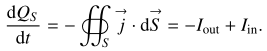 (1)
(1)
One assumes that the control surface is close enough to the spacecraft surface, such that the spacecraft potential is to a good approximation proportional to the charge QS. The variation in the spacecraft potential can then be associated with the action of different currents, Iin and Iout, through the surface, S. Now one also assumes the control surface to be large enough for all the charge generated by impact ionization just after the dust hit to be initially enclosed by it: then, there is no variation in the charge inside the surface and therefore no variation in potential in the first moments after the impact. At that point, some electrons may escape out of the control surface: associated with this escape will be a negative outward current and then a positive voltage pulse (the “electron precursor”) in the spacecraft potential times series. In a second time, ions crossing the control surface will then produce a positive outward current and, therefore, a negative drop in the spacecraft potential. Finally, on the longest timescale, currents from the solar wind and photoelectron emission from the spacecraft will lead to the relaxation of the voltage pulse. These correspond to the three stages of the voltage pulse as described by Mann et al. (2019) (T2, T3 and T4 in that paper). This approach is mathematically relevant, and has the advantage of simplicity and pragmatism. On the other hand, it is not fully satisfactory since it leaves the processes occurring inside the control surface undescribed. For instance, it is clear that it is not the crossing of a mathematically abstract – and loosely defined – control surface by electrons or ions that is responsible for the spacecraft potential changes. The changes are physically produced by the collection of, and by the influence from, charges inside the control surface. Another drawback of this approach is that the currents associated with the cloud dynamics appear as ad hoc functions, which are difficult to link to the specific spacecraft geometrical properties.
This motivates our study. In the following, we focus on the case of the positively charged STEREO spacecraft, although the model can of course easily be extended to all spacecraft’s charging states and processes. We provide a model that accounts for the collection of negative charges and the exchange of charges with the surrounding solar wind plasma, as was done in Zaslavsky (2015). Here we add to the picture the effect of the electrostatic influence from the positive ion cloud and therefore recover the “slow rise time” and voltage precursor effects, that were absent from that work.
2.2. Electrostatic influence from a point charge
The electrostatic potentials of a system of conductors insulated from one another is a problem that, although not explicitly solvable for arbitrary geometries, has the advantage that the charge carried by each of the conductive elements is linear. Considering our system to be composed of only the dust plasma cloud, of charge Qcloud and potential φcloud, and the spacecraft (indices sc), the linearity of the problem translates into the existence of a matrix Λ such that
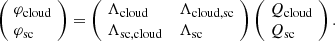 (2)
(2)
Here, Λ is here the inverse of the capacitance matrix, also known as the elastance matrix, of the conductors system. Of course, additional lines and columns can be added in order to account for the electrostatic effects of the dust on other systems (antennas, solar panels, booms, etc.) and of these elements on each other, but in this paper we focus only on the simplest case of the interaction of a dust impact cloud and the spacecraft, neglecting all other capacitive couplings and therefore limiting ourselves to a 2 × 2 matrix. This choice is made here for simplicity, but a model that includes the coupling to the antennas should be the purpose of a forthcoming study. This would be of particular importance in providing a model for the signals observed in dipole mode on Wind and other spacecraft (Solar Orbiter, Parker Solar Probe), which are known to be produced by electrostatic influence on a particular arm of a dipole (Meyer-Vernet et al. 2014).
Since the size of the spacecraft is very large with respect to the size of the dust impact cloud that influences it (so its self-capacitance is much larger), we can neglect the change in self-capacitance of the spacecraft due to the presence of the cloud in its vicinity and write that
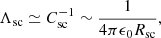 (3)
(3)
where Csc is the spacecraft capacitance in a vacuum and Rsc its size. This parameter is then a good approximation independent of the position of the dust cloud with respect to the spacecraft.
In order to roughly evaluate Λsc, cloud, one could assume the dust cloud to be a point charge and the spacecraft to be a conducting sphere of radius Rsc, both separated by a distance r. The electrostatic calculation in a vacuum (see e.g., Jackson 1962), as noted by Meyer-Vernet et al. (2017), then gives
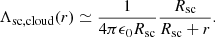 (4)
(4)
This evaluation neglects lots of effects, especially the fact that the dust-spacecraft interaction does not occur in a vacuum, and that the interaction potential is screened by the photoelectron sheath. Therefore, we chose to model the mutual elastance, Λsc, cloud, by
 (5)
(5)
where F(r) is a decreasing function (with a typical length scale, λph, the screening length of the photoelectron sheath), with limiting values of 1 for r → 0 and 0 for r → ∞. Naturally, one may choose
 (6)
(6)
but other empirical choices are possible – for instance, F(r)∝exp(−r/λph)/(r + Rsc), to recover the vacuum expression given by Eq. (4) for small values of r. The function F has to be chosen empirically anyway since it depends on many indeterminate factors, including the geometry of the spacecraft, the geometry of the dust impact cloud, and the structure of the photoelectron sheath.
2.3. Equations for the potential perturbation
Now that we have our model for the electrostatic influence, we can study the effect on the spacecraft potential of a transient as a dust impact. For this we use Eq. (2) to write the derivative of the spacecraft potential,
 (7)
(7)
The first term of the right-hand side accounts for the time variation of the spacecraft charge. This variation is due to various currents coming from the dust impact cloud, the solar wind plasma and the spacecraft itself through the photoelectric effect (or, very marginally in the case of STEREO, secondary emission). It corresponds to the variation in charges in a control volume that is precisely enclosed by the spacecraft’s surface. It reads (neglecting secondary emission)
 (8)
(8)
where Iph is the photoelectron current and Isw is the solar wind electron current on the spacecraft surface, which can both be expressed explicitly as a function of φsc (and of the local plasma parameters) within the orbit-limited approximation (Laframboise & Parker 1973). The Icollected(t) is the current due to collected charges from the impact cloud. This equation (that is, Eq. (7) with only the first term of the right-hand side) corresponds exactly to what was solved in the paper by Zaslavsky (2015). It captures the effects related to the changes in the charge carried by the spacecraft: its charging through collection of charges from the impact cloud and its relaxation to equilibrium through charge exchanges with the solar wind. The second term of the right-hand side of Eq. (7) was omitted from that paper, but it is very important: it contains the description of the effects of electrostatic influence.
The solution of Eq. (7) can be obtained by linearizing the expression for the currents around the equilibrium value, φsc, eq, of the potential, as was done in Zaslavsky (2015). The potential perturbation, δφsc = φsc − φsc, eq, is then found to evolve according to the first-order linear differential equation
![Mathematical equation: $$ \begin{aligned} \frac{\mathrm{d}}{\mathrm{d}t} \delta \varphi _{\rm sc} + \frac{1}{\tau _{\rm sc}} \delta \varphi _{\rm sc} = \frac{1}{C_{\rm sc}} \left( I_{\rm collected} + \frac{\mathrm{d}}{\mathrm{d}t} \left[ F(r(t)) Q_{\rm cloud}(t) \right] \right), \end{aligned} $$](/articles/aa/full_html/2022/03/aa42508-21/aa42508-21-eq9.gif) (9)
(9)
where τsc is the linear relaxation time of the spacecraft potential
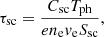 (10)
(10)
with Tph the photoelectron sheath temperature expressed in electronvolts, ne the local plasma electron density, 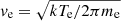 the electron mean velocity divided by 4, Te the local plasma electron temperature and Ssc the spacecraft conductive surface in contact with the surrounding plasma. The k, e and me are Boltzmann’s constant, the electron charge, and the electron mass, respectively. The solution of Eq. (9), assuming the spacecraft is in equilibrium with the surrounding plasma when t → −∞, is
![Mathematical equation: $$ \begin{aligned} \begin{aligned} \delta \varphi _{\rm sc}(t) = \frac{1}{C_{\rm sc}} e^{-t/\tau _{\rm sc}} \int _{-\infty }^{t} \left( I_{\rm collected}(t^\prime ) + \frac{\mathrm{d}}{\mathrm{d}t^\prime } \left[ F(r(t^\prime )) Q_{\rm cloud}(t^\prime ) \right] \right) \\ e^{t^\prime /\tau _{\rm sc}} \mathrm{d}t^\prime . \end{aligned} \end{aligned} $$](/articles/aa/full_html/2022/03/aa42508-21/aa42508-21-eq12.gif) (11)
(11)
This expression can be used in a quite general manner to model the shape of the pulse – as long as the linear assumption is fulfilled, which is the case for the very large majority of the impacts recorded. One can see that the time profile of the voltage perturbation is linked to the time profile of the collected current, Icollected, but also to the trajectory, r(t), of the dust cloud around the spacecraft, to the shape of the function F, describing the spacecraft and sheath properties, and to the time profile Qcloud(t), which is related to the electron dynamics in the cloud and in the sheath.
2.4. A simple model: Streaming ions and massless electrons
In order to obtain a simple model, that relies on a few parameters and is adapted to robust fitting of the large amount of data provided by radio instruments such as S/WAVES, one needs models to be as simple as possible for the source terms in the right-hand side of Eq. (11). We derive in this section the potential perturbation time profile under the simple assumption that the ions are streaming out of the spacecraft surface with a constant velocity, v, and that the motion of the electrons occurs fast enough that it can be considered as instantaneous. This assumption is relevant if the electron dynamical timescale is smaller than the sampling time of the instrument, which is the case, as will be seen in the data analysis section, for the waveforms recorded by S/WAVES. We also consider the possibility that the photoelectrons in the sheath neutralize the ion cloud, since this effect was shown to be important by Meyer-Vernet et al. (2017).
For the function F – which is proportional to the mutual elastance of the cloud-spacecraft system, we use the exponential model Eq. (6) with a cutoff length λph on the order of the photoelectron sheath Debye length. Since we consider ions streaming freely out of the spacecraft, the spacecraft-ion cloud distance is given by r(t) = vt, with v a constant.
Therefore, the term accounting for electrostatic influence reads
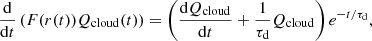 (12)
(12)
where τd = λph/v is the ion cloud dynamics timescale, characteristic of its transit time (or expansion time) in the photoelectron sheath. Now one must model the effects related to the motion of the cloud’s electrons. For this, we use the following equation, which expresses the change in the cloud’s charge due to currents of electrons from it and the neutralization of the cloud by the photoelectrons on a typical timescale τph:
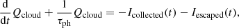 (13)
(13)
where Iescaped is the current of charges escaping away from the spacecraft.
The assumption that the escape and collection of the electrons is instantaneous (the “massless electron assumption”) translates into the following expressions for the currents
 (14)
(14)
where Q > 0 is the total amount of free charges released in the impact ionization process, ϵ is the fraction of electrons escaping away from the spacecraft, and δ(t) is Dirac’s delta function. It is then clear that one must have, from the Eq. (13),
 (15)
(15)
where H(t) is Heaviside’s step function.
All the source terms appearing in the right-hand side of Eq. (11) have now been given by an explicit expression, and it is straightforward to compute the integral. The potential perturbation obtained is
![Mathematical equation: $$ \begin{aligned} \delta \varphi _{\rm sc}(t) = \left[ \frac{\epsilon Q}{C_{\rm sc}} e^{-t/\tau _{\rm sc}} - \frac{Q}{C_{\rm sc}} \frac{1}{1-\tau _i/\tau _{\rm sc}}\left( e^{-t/\tau _{\rm sc}} - e^{-t/\tau _{i}} \right) \right] H(t). \end{aligned} $$](/articles/aa/full_html/2022/03/aa42508-21/aa42508-21-eq17.gif) (16)
(16)
where τi = τdτph/(τd + τph) is the characteristic rise time of the pulse. It is on the order of the smaller of the ion characteristic timescale, τd, and the time for the cloud to collect enough ambient photoelectrons to be able to shield its charge, Q (Meyer-Vernet et al. 2017).
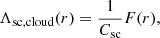
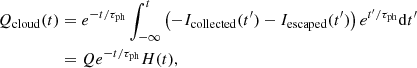
The shape of this time profile is illustrated in Fig. 1. In the case where the ion timescale, τi, is small compared to the relaxation time, τsc, this can easily be simplified again, but we keep the effect of the finite value of τi/τsc, since, as we shall see, in the data this ratio is on the order of ∼1/3.
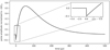 |
Fig. 1. Simulation of the signal shape through proposed models for the effect on the spacecraft potential of a transient dust impact. The curve is obtained from the simple model, assuming the electron collect (escape) to be instantaneous, τe ≈ 0 (Eq. (16)). The ratio between escaped charge and total charge is ϵ = 0.1, and timescales parameters are τsc = 100 μs and τion = 30μs. The zoomed-in portion of the plot (top right) provides an insight into the pre-shoot signal shape. |
2.5. More complicated model: Taking additional effects into account
The previous section presents a simple model, which, as will be seen in the next section, is sufficient for modeling and understanding the broad majority of the events recorded by S/WAVES. But the expression (11) for δφsc(t) also makes it possible to account for a variety of other effects, by introducing more refined functions for the collection (escape) currents, the mutual elastance, or the ion cloud trajectory. In this section we briefly explore some possible refinements.
First, one could account for the finite dynamic time, τe, of the electrons. This can be done by using for Icollected and Iescaped functions that introduce a characteristic timescale. The most natural choice is probably a Gaussian function with variance  . In general, it will then be necessary to perform a numerical integration of the Eqs. (11) and (15). If it is necessary to reach an even finer level of modeling for the electron dynamics, one could also take different timescales for the collection and escape of the electrons into account. Of course, such a fine modeling given the time resolution of the electric waveform sampler on board spacecraft, would probably not make much sense in the context of space measurements.
Another refinement could also be obtained by accounting for more complex trajectories, r(t), of the ion cloud. Here again, the computation for an arbitrary trajectory requires numerical integration. In any case, and as will be seen in the next section, since the screening timescale, τph, is smaller than the dynamics timescale, τi, the precise dynamics of the ion cloud should not strongly affect the shape of the pulse.
Finally, a finer description of the pulses could also be reached through a better modeling of the spacecraft coupling to the cloud. Such a model should include a precise electrostatic description of the spacecraft through a carefully computed elastance matrix that includes all the conductive elements and in particular the antennas, the potential of which was considered as constant in our simplified study. The computation of such an elastance matrix was recently performed by Shen et al. (2021) and compared to the results of laboratory experiments of dust impacts on a model spacecraft.
A full model may also include a description of the cloud internal dynamics and expansion and of the trajectory vector, r(t), of the cloud center of mass in the vicinity of the spacecraft. Solving for such a complicated model would require complex numerical simulations. But as we shall see in the next section, the present model enables us to reproduce most of the observed voltage pulses and provides a support for interpreting the more complex ones.
3. S/WAVES Time Domain Sampler data
In the present study, we analyze dust grain impacts from the two STEREO satellites, A and B, which were launched in 2006 and are orbiting at 1 AU. The S/WAVES radio instrument is constituted by three orthogonal 6 m long antennas connected to a sensitive radio receiver. The instrument can perform observations in the frequency range 2.5 kHz to 17 MHz (Bale et al. 2008; Bougeret et al. 2008). The Time Domain Sampler (TDS) is a subsystem of the S/WAVES instrument that generates high-cadence time series of voltage pulses for each monopole. Bougeret et al. (2008) provided comprehensive information on TDS and how signals are collected, filtered, and digitized. In this article, we use the data provided by TDS to study the voltage variations occurring when a dust grain impacts the spacecraft.
3.1. Presentation of S/WAVES TDS data
Two TDS data sets are available: (1) the TDSmax data give the maximum amplitude or peak signal detected on the antennas each minute; and (2) the TDS Events data set provides complete voltage time series captured by the instrument with a sampling rate of a few μs (Zaslavsky et al. 2012). We used the TDS Events data set. Measurements can be conducted in several modes with different time resolution and total event duration. For this study snapshots with a time resolution of 4 or 8 ms (which constitute the vast majority of the signals) are used. They correspond to snapshot durations of 65 ms and 130 ms. Signals with a high amplitude are automatically selected for telemetry out of a continuously recorded waveform. A low-pass filter is used with the S/WAVES signal to prevent aliasing by matching the sampling channel. Depending on the time resolution of the sample, low-pass filters can be either 108 kHz or 54 kHz (Bougeret et al. 2008).
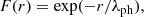
An analysis of the electrical waveforms of the TDS Events reveals that they contain a variety of signals with distinctly different shapes. The observed signals include variations in electric potential due to inhomogeneities of local plasma density. Panels a–c of Fig. 2 illustrate the types of waves present in the data: plasma waves oscillating at the local plasma frequency (Langmuir waves), plasma waves around the local cyclotron frequency, and low-frequency density fluctuation. The impact of energetic particles such as protons and electrons from the Solar System or coming from galactic origin can also produce an electric field signal. All these signals are well known and have been the subject of many works (e.g, Kellogg et al. 1996; Bale et al. 1998; Henri et al. 2011; Malaspina et al. 2011). Panel d of Fig. 2 shows a signal of characteristic shape recognized as a dust impact signal (Zaslavsky et al. 2012). This signal is characterized by an abrupt increase in voltage followed by a rapid relaxation to equilibrium potential. There are two distinct types of these signals: a strong peak detected by one monopole or a similarly shaped signal appearing simultaneously on all three antennas. Our study is focused on signals almost simultaneously generated on all three antennas.
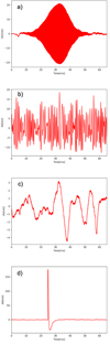 |
Fig. 2. Different examples of electrical signals obtained by S/WAVES/TDS: (a) Langmuir waves, (b) plasma wave around the local cyclotron frequency, (c) low-frequency density fluctuation, and (d) dust event. |
3.2. Survey of TDS dust data
The TDS waveform sampler on-board both STEREO satellites has observed a large number of voltage pulses interpreted as dust impact signatures since the launch of the mission. Our study examines TDS events recorded from 2007 to 2018 for STEREO A and from 2007 to 2015 for STEREO B.
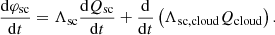
As illustrated by Fig. 2, the data set contains snapshots of a wide variety of phenomena. Therefore, we need to find a way to automatically identify only very sharp and impulsive events, recognized as dust events, in between all those other varieties of occurrences. To do so, we set the threshold at an amplitude greater than 15 mV to identify shapes clearly and lower than 175 mV to eliminate events that saturate the receiver. Also, since we wanted the amplitude to be roughly the same on all three antennas, our third criterion is defining a cone that will only involve simultaneously occurring. Figure 3 shows the distribution of the observed maximum amplitudes over three months on the monopole pair X and Y (the distribution is the same for the other monopole pairs). Accordingly, if we consider measurements of each of the three monopoles, dust events would likely be concentrated within the cone of a particular aperture. In parallel with dust events, we have also detected Langmuir waves with a corresponding amplitude. Insofar as we limit the signal to just two points at an intersection of one-third of the height of the maximum amplitude, we eliminate all Langmuir waves from our obtained dust database. An auto-detection algorithm that meets all the above criteria was tested using three months of observations over which several dozen measurements of dust impacts were made; it was found to be effective in detecting dust-related events. Then we applied it to the entire TDS Events data set.
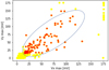 |
Fig. 3. Maximum signal amplitude recorded on X and Y monopoles in the period from 2008 October 1 to 2008 December 31. Red stars represent only the dust signal. |
We have gathered all dust events measured on all three monopoles simultaneously with maximum amplitudes between 15 and 175 mV from the TDS Events data set in 2007–2018 to create a single database. The resulting database contains 116544 events, 76086 on STEREO A and 40458 on STEREO B. In order to check the validity of the simple theoretical model presented in Sect. 2, a statistical analysis based on the events in the database was conducted. Due to the fact that each impact creates a pulse on each of the three monopoles, there are 349632 individual pulses.
3.3. Analysis of individual impacts
Using the simple model from Sect. 2, we fitted each electric pulse observed by the S/WAVES instrument on board STEREO A and B, selected as discussed in Sect. 3.2. Several parameters that characterize the response of the spacecraft and the collection dynamics of particles are derived and discussed. To fit the signal detected at each monopole, we used the function
 (17)
(17)
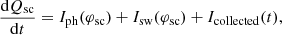
with a Levenberg-Marquardt least-squares minimization method. This function is the same as the theoretical Eq. (16), with the free parameters of our fitting routine being: T2 ≡ τsc is the spacecraft relaxation timescale, which is the time it takes for the spacecraft to return to equilibrium; T1 ≡ τi is the ion characteristic timescale, A ≡ ΓQ/Csc is the total charge, and B ≡ ϵΓQ/Csc represents the escaped charge. Figure 4 shows voltage pulses recorded by TDS as well as the Levenberg-Marquardt fit to TDS data with the function δV(t) = − Γδφsc from Eq. (17), with Γ ∼ 0.5 the antennas’ gain due to capacitive coupling with the base (Bale et al. 2008). These examples demonstrate a good match between the data and the model, except for the negative voltage overshoot occurring after the main pulse.
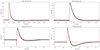 |
Fig. 4. Signals of dust impact recorded by STEREO A in 2008. Black dots represent TDS data. The red line represents the fitting results made with a Levenberg-Marquardt method from Eq. (17) and function δV(t) = − Γδφsc. |
As discussed in the previous subsection, anti-aliasing low-pass filters are set up at the entrance of each sampling channel. It is known that the effect of such filters on a sharp impulsive signal will produce an artificial distortion of the signal, such as these overshoots. In order to correct this effect, we deconvolved the signal using the inverse low-pass filter. The inverse low-pass filter was chosen in accordance with the sampling channel currently being used, which is typically 108 kHz or 54 kHz in the case of S/WAVES (Bougeret et al. 2008). Some overshoots remain even after the correction, while others completely disappear. It is therefore likely that the remaining overshoots are not artificial, but rather due to the charges of the monopoles themselves (Zaslavsky 2015). Still, this effect is difficult to reliably quantify since the correction by the filter can be quite sensitive to the phase calibration of the filters. In this study, we chose not to take the variation in the antenna’s potential into account.
As a summary, we fitted all data from our data base with the Levenberg-Marquardt least-squares minimization method using Eq. (17). As discussed in Sect. 2, we expect that the time required for the spacecraft to return to equilibrium is significantly longer than the ion characteristic timescale (i.e., τsc > τi). We removed any event that does not meet this condition; consequently, from the initial 349632 events, we kept about 70% of the events.
3.4. Statistical analysis of S/WAVES signals, presentation and discussion
3.4.1. Linear relaxation timescale
Figure 5 shows a histogram of the parameter τsc, which describes the discharge timescale of the spacecraft through exchange of charges with the solar wind and the photoelectron emission from the spacecraft. The histogram contains all the values for the τsc parameter that were obtained for each monopole.
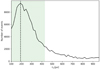 |
Fig. 5. Histogram of the parameter τsc. The green section on the histogram indicates the extreme values of the parameter calculated from Eq. (10) (see text for details). Around 80% of the obtained values for τsc are inside the green section. The dashed vertical line represents the most probable obtained value for the parameter, τsc ∼ 190 μs. The median value of the distribution is 270 μs. |
The linear relaxation time of a spacecraft is given by Eq. (10) in Sect. 2.3. One can see that τsc depends on the geometry of the spacecraft (through its surfaces), as well as on the local plasma and photoelectron parameters. It can be evaluated as follows: STEREO satellites orbit at 1 AU, where, typically, ne ≃ [1 − 10] cm−3 and Te ∼ 10 eV (Issautier et al. 2005). Spacecraft parameters are, as an order of magnitude, Csc ≃ 200 pF, Ssc ≃ 10 m2, and the photoelectron temperature is typically Tph ≃ 3 eV. On the basis of these parameters, one can estimate the relaxation time for STEREO, τsc ∼ 100 − 430 μs. These limits are represented by the green-shaded area in Fig. 5. One can see that the distribution of the observed relaxation times peaks roughly in the middle of the green area and that most of the data (∼80%) fall within the expected range. The most probable value and median observed values are 190 μs and 270 μs, respectively. This quite unambiguously shows that, consistent with the standard interpretation, the decay time of the pulses can be identified with the relaxation time of the spacecraft through the exchange of charges with the surrounding plasma after the spacecraft body has collected a certain amount of charge.
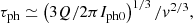
3.4.2. Ion characteristic timescale
Figure 6 presents a histogram of the ion dynamics timescale parameters, τi. The vast majority of the obtained values for parameter τi are smaller than 100 μs. As noted in Sect. 2.2, this characteristic ion timescale, τi, is the smallest of the quantities λph/v and the time for the cloud’s ions to collect enough ambient photoelectrons to be shielded by them, as estimated by Meyer-Vernet et al. (2017). Using Eqs. (11) and (4) of that paper, the latter can be simplified into
 (18)
(18)
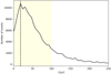 |
Fig. 6. Histogram of the parameter τi. The yellow section includes all the obtained values below 100 μs (the threshold for the τsc). More than 80% of the obtained τi is inside the yellow section. The vertical dashed line represents the most probable obtained value for the parameter, τi ∼ 18 μs. |
where Iph0 is the spacecraft photoelectron current at zero potential. Assuming Iph0 ≃ 20 μA/m2 (which yields λph ≃ 0.9 m), we deduce from the most commonly observed value τi = 18 μs (Fig. 6) with the average charge Q ≃ 40 pC, the cloud’s propagation and expansion speed to be v ≃ 13 km s−1. This result depends weakly on the badly known photoelectron current and is consistent with our estimate that τi ≃ τph since the most commonly observed value of τi is much smaller than λph/v.
These values can be compared with reasonable agreement to measurements from laboratory experiments and numerical simulations. For instance, our results match those of Lee et al. (2012), who measured the ion expansion speed in laboratory experiments and found v ≥ 10 km s−1. According to their results, plasma detection occurred most often from impacts on positively charged targets (such as STEREO). In contrast, detection rates for negatively charged and unbiased targets varied depending on the material. Based on multi-physics simulations of plasma production from hypervelocity impacts, Fletcher et al. (2015) reported a similar range of values.
3.4.3. Electron collection
The value of total charge, Q, is derived from the parameter A ≡ ΓQ/Csc, which is obtained through the fitting. It should be noted that the value of A obtained on each monopole differs a bit (probably because of the influence effect on the monopoles, which is neglected in this work). However, since the total amount of charge released during an impact must be the same for all monopoles, we defined the total charge as the mean of the values obtained by fitting each monopole separately. For both STEREO spacecraft we used values for the spacecraft capacitance of Csc= 200 pF, and for the antenna-spacecraft coupling Γ ≃ 0.5 (Bale et al. 2008). As can be seen in the figure, values of Q lie within the range 8–120 pC.
The link between the total charge generated Q, and both the mass, m, and velocity, V, of the impacting dust particles with respect to the spacecraft was studied recently using hypervelocity impact experiments on materials relevant to STEREO satellites (Collette et al. 2014). In the case of impacts on the thermal coating that covers most of the spacecraft, the result obtained is Q[C] ≃ 1.7 × 10⁻³ ![Mathematical equation: $ \mathrm{m_{[kg]}} V^{4.7}_{[\mathrm{km.s^{-1}}]} $](/articles/aa/full_html/2022/03/aa42508-21/aa42508-21-eq21.gif) . Based on this relationship, we can, by assuming a typical velocity for the impacts, translate the charge scale into a mass scale. For particles orbiting at Keplerian speeds, we can assume a typical impact velocity of 30 km.s−1; the obtained mass range is then 20 − 340 × 10−17 kg, which corresponds to the size interval 2 – 5 μm (we assume a mass density ρ = 2.5 g.cm−3 ). On the other hand, it has appeared that the fluxes observed on several spacecraft, including STEREO (Zaslavsky et al. 2012), but also Parker Solar Probe (Pusack et al. 2021) and Solar Orbiter (Zaslavsky et al. 2021), are dominated by impacts from a population of dust particles produced close to the Sun and pushed away along hyperbolic orbits by the radiation pressure, the β meteoroids. The velocity of these particles at 1 AU depends quite importantly on their origin and composition, through the value of the β parameter equal to the ratio of the radiation pressure force to the gravitational force on the dust grain. For dust of asteroidal origins, an order of magnitude of the velocity at 1 AU is 80 km.s−1 (Wilck & Mann 1996). Using this value we obtain masses and sizes ranging from 0.4 to 6 × 10⁻¹⁷ kg, and from 0.07 to 0.17 μm, respectively, which is comparable to the masses and sizes of grains detected on the cited missions.
. Based on this relationship, we can, by assuming a typical velocity for the impacts, translate the charge scale into a mass scale. For particles orbiting at Keplerian speeds, we can assume a typical impact velocity of 30 km.s−1; the obtained mass range is then 20 − 340 × 10−17 kg, which corresponds to the size interval 2 – 5 μm (we assume a mass density ρ = 2.5 g.cm−3 ). On the other hand, it has appeared that the fluxes observed on several spacecraft, including STEREO (Zaslavsky et al. 2012), but also Parker Solar Probe (Pusack et al. 2021) and Solar Orbiter (Zaslavsky et al. 2021), are dominated by impacts from a population of dust particles produced close to the Sun and pushed away along hyperbolic orbits by the radiation pressure, the β meteoroids. The velocity of these particles at 1 AU depends quite importantly on their origin and composition, through the value of the β parameter equal to the ratio of the radiation pressure force to the gravitational force on the dust grain. For dust of asteroidal origins, an order of magnitude of the velocity at 1 AU is 80 km.s−1 (Wilck & Mann 1996). Using this value we obtain masses and sizes ranging from 0.4 to 6 × 10⁻¹⁷ kg, and from 0.07 to 0.17 μm, respectively, which is comparable to the masses and sizes of grains detected on the cited missions.
Figure 7 shows the total charge, Q, obtained through the fitting procedure, as a function of the charge Qestimate estimated with the approximation Qestimate = CscδVmax/Γ – the formula that has been used for several space missions (e.g., Zaslavsky et al. 2012) when waveform data are not available for each event. Figure 7 shows that this rough estimate is very well correlated with the total charge, Q, deduced from fitting the waveform. The slope is 1.63 ± 0.01, with 0.8 the factor of correlation. This high correlation justifies the use of the formula A ≡ ΓQ/Csc when no precise waveform data are available. However, this study shows that this formula underestimates the charge by around 30% (at 1AU).
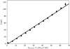 |
Fig. 7. Total charge calculated from Qestimate = CscδVmax/Γ as a function of the total charge, Q, obtained from fitting parameter A (Eq. (17)). The binwidth is 5 pC. The error bars show the standard deviation of the distribution of Q in each bin. |
This underestimation has had some consequences on the estimation of particle size, in previous studies (e.g., Zaslavsky et al. 2012). Since we have seen that size is linked to Q by s ∝ Q1/3, we can estimate that the size, s, must be underestimated by around 10% – which is quite small given all the other sources of uncertainties.
3.4.4. Electron escape
We finally turn our attention to the electron escape current. Figure 8 shows value of the amount of charge escaping the spacecraft, ϵQ, as a function of the estimated total cloud charge, Q. The standard deviation shown as error bars gives an estimate of the width of the distribution of escaped charge in each bin. For this figure we choose only events exhibiting a voltage precursor larger than 5 mV. Our database contains about 20% of such events. Figure 9 shows the percentage of events with precursor amplitude larger than the threshold concerning the total charge amount Q.
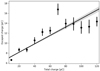 |
Fig. 8. Escaping charge, ϵQ, as a function of the total charge released in the cloud, Q. The points show the average of the values of ϵQ per bins of values of Q. The binwidth is 10 pC. The error bars show the standard deviation of the distribution of ϵQ in each bin. |
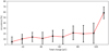 |
Fig. 9. Histogram of the occurrence of events with precursor amplitude larger than 5 mV with respect to the total charge amount. The error bars show the standard deviation of the distribution. The binwidth is 12 pC. |
Figure 8 shows that both are almost linearly correlated (at least up to 70 pC), implying that the fraction of escaping charge, ϵ, is almost a constant. The slope of the curve, obtained by linear regression, provides a value of ϵ = 0.085 ± 0.004, where the uncertainty correspond to a 95% confidence interval on the value of the slope.
To our knowledge, this is a novel result. It shows that, on average and pretty much independently of the total amount of charge in the cloud, around 8% of this charge escapes the spacecraft. This offers, for instance, a way to evaluate at least an order of magnitude of the amount of charge released during an impact that saturates the instrument if a precursor is associated with this event.
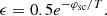
This result has a further interesting consequence. It enables us to estimate the temperature of the impact-produced electrons as follows. Roughly half of such electrons are expected to move toward the spacecraft initially and recollected, provided the spacecraft potential is positive. Among the other half (those initially moving outward), only those with an energy (in eV) exceeding the spacecraft potential, φsc, will escape. Assuming a Maxwellian distribution of temperature T (in eV), this yields
 (19)
(19)
With ϵ ≃ 0.08 and φsc = 5 V, we obtain T = 2.7 eV. This result is close to the value T = 2.5 eV found by Fletcher et al. (2015) and to all the previous estimates, which indicated that the impact electron temperature is a few eV.
Recently, impulsive magnetic signals have been detected by search coils associated with very large amplitude (saturating) signals on the monopoles of Parker Solar Probe and Solar Orbiter (T. Dudot de Wit, M. Kretzschmar, priv. comm.). Such signals are likely produced by the current generated by electrons escaping from the spacecraft. In this context, our measurement takes on a supplementary interest since it help us to evaluate the escaping current from the amplitude of the pre-shoot. Indeed, one must have Iescape ∼ ϵQ/τe, where τe is the timescale associated with the electron dynamics. As discussed previously, this timescale has been neglected (τe ∼ 0) in the present study. This was justified by the fact that in nearly every case the rise time of the voltage precursor is not time-resolved by the TDS instrument, even when it is functioning at it highest time resolution of 4 μs. Therefore, this time resolution can be safely considered as a higher limit on τe, and one can evaluate
 (20)
(20)
The amplitude of the magnetic pulses must be on the order of δB ∼ μ0Iescape/2πR, with R the average distance between the outflowing electrons and the magnetic probe. We can then expect the amplitude of the magnetic pulse to be linearly related to the amplitude of the voltage precursor. Checking the linearity of this relation on a statistically relevant set of observed magnetic pulses would provide an interesting test for the hypothesis that the magnetic pulses are indeed produced by the current of escaping electrons.
Moreover, one can use the value of the parameter ϵ derived from our observations to estimate the size of the dust that produce magnetic pulses. For instance, an escaping current that produces a magnetic pulse of amplitude Bobs ∼ 0.5 nT, taking for R a value typical of the spacecraft size, ∼1 m, should be Iescape ∼ 2πRscBobs/μ0 ∼ 3 mA. Now assuming that the value of ϵ stays constant ∼0.08 even for large values of Q, this current would correspond to a total impact charge of Q ∼ Iescapeτe/ϵ ∼ 100 nC. For impact speeds of 50 – 100 km.s−1 (relevant for Solar Orbiter and Parker Solar Probe; cf. Page et al. 2020), this would give masses of m ∼ 10−14 kg or sizes of a few microns. This is an interesting test for the hypothesis that the magnetic pulses are indeed produced by the current of escaping electrons.
4. Conclusions
-
In this study we present a theoretical model for the generation of voltage pulses by the collision of dust grains onto a spacecraft. Our work, in the continuation of previous studies (Zaslavsky 2015; Meyer-Vernet et al. 2017), provides for the first time an analytical formula describing the voltage pulse as a consequence of the combined effects of charge collection by the spacecraft and electrostatic influence from charges in its vicinity. We validate our model using data from the S/WAVES instrument at 1 AU.
-
We used the S/WAVES TDS instrument to determine the four independent free parameters appearing in our model (total ion charge, Q, fraction of escaping charge, ϵ, rise timescale, τi, and relaxation timescale, τsc) by fitting our model to the waveform data using a least-square Levenberg-Marquardt technique. This enabled us to obtain the first in situ measurements of parameters such as the electron escape current and the temperature of the electrons in the impact cloud (T ∼ 2.5 eV).
-
Our study is consistent with the idea that the pulse’s rise time largely exceeds the spacecraft’s short timescale of electron recollection. When the electrons are recollected, the positive ions are still very close to the spacecraft since mi ≫ me. Hence, they produce a voltage of the opposite sign to that produced by the electron recollection. Therefore, the rise time of the signal is determined by the voltage induced on the spacecraft by the cloud’s positive ions (Meyer-Vernet et al. 2017). Moreover, obtained values for the rise time give us insight into the propagation speed of the ion cloud. As far as we know, this is the first time that information about the velocity of ion clouds was calculated from data, and we compared the results with the values obtained in numerical simulations and laboratory instruments. Calculations based on numerical simulations (Fletcher et al. 2015) and laboratory experiments (Lee et al. 2012) match our results.
-
We found that the amount of charge escaping the spacecraft and the estimated total cloud charge are almost linearly correlated. Recently detected impulsive magnetic signals associated with saturating signals on the monopoles of Parker Solar Probe and Solar Orbiter are likely related to the electrons escaping from the spacecraft. In this context, our model takes on a supplementary interest since it helps us evaluate the escaping current from the amplitude of the precursor.
-
The effect of the potential induced by the cloud’s ions on the antennas, expected to be small on STEREO, could explain the minor differences between the voltages measured on the three monopole antennas. However, on other missions where the antennas are located on different sides of the spacecraft, for example WIND, Parker Solar Probe, and Solar Orbiter, this effect should produce very different voltages on different antennas and therefore enable dust detection in dipole mode, as first suggested by Meyer-Vernet et al. (2014).
Acknowledgments
We thank the team who designed and built the S/WAVES instrument. The S/WAVES data used here are produced by an international consortium of the Observatoire de Paris (France), the University of Minnesota (USA), the University of California Berkeley (USA), and NASA Goddard Space Flight Center (USA). All the analysis was done, and the plots produced using open source PYTHON libraries NUMPY, MATPLOTLIB, PANDAS, and SCIPY. The French contribution is funded by CNES and CNRS. During the work on this paper KRB and DO was financially supported by the Ministry of Education, Science and Technological Development of the Republic of Serbia through the contract No. 451-03-9/2021-14/200104. AZ acknowledges discussions during the ISSI team on dust impacts at the International Space Science Institute in Bern, Switzerland.
References
- Aubier, M. G., Meyer-Vernet, N., & Pedersen, B. M. 1983, Geophys. Rev. Lett., 10, 5 [NASA ADS] [CrossRef] [Google Scholar]
- Bale, S. D., Kellogg, P. J., Larsen, D. E., et al. 1998, Geophys. Rev. Lett., 25, 2929 [NASA ADS] [CrossRef] [Google Scholar]
- Bale, S. D., Ullrich, R., Goetz, K., et al. 2008, Space Sci. Rev., 136, 529 [NASA ADS] [CrossRef] [Google Scholar]
- Bougeret, J. L., Kaiser, M. L., Kellogg, P. J., et al. 1995, Space Sci. Rev., 71, 231 [CrossRef] [Google Scholar]
- Bougeret, J. L., Goetz, K., Kaiser, M. L., et al. 2008, Space Sci. Rev., 136, 487 [CrossRef] [Google Scholar]
- Collette, A., Grün, E., Malaspina, D., & Sternovsky, Z. 2014, J. Geophys. Res. (Space Phys.), 119, 6019 [NASA ADS] [CrossRef] [Google Scholar]
- Collette, A., Meyer, G., Malaspina, D., & Sternovsky, Z. 2015, J. Geophys. Res. (Space Phys.), 120, 5298 [NASA ADS] [CrossRef] [Google Scholar]
- Fletcher, A., Close, S., & Mathias, D. 2015, Phys. Plasmas, 22, 093504 [NASA ADS] [CrossRef] [Google Scholar]
- Gruen, E., Fechtig, H., Kissel, J., et al. 1992, A&AS, 92, 411 [NASA ADS] [Google Scholar]
- Grün, E., & Dikarev, V. 2009, Landolt Börnstein, 4B, 644 [Google Scholar]
- Gurnett, D. A., Grun, E., Gallagher, D., Kurth, W. S., & Scarf, F. L. 1983, Icarus, 53, 236 [NASA ADS] [CrossRef] [Google Scholar]
- Gurnett, D. A., Ansher, J. A., Kurth, W. S., & Granroth, L. J. 1997, Micron-Sized Dust Particles Detected in the Outer Solar System by the Voyager 1 and 2 Plasma Wave Instruments, National Aeronautics and Space Administration Report [Google Scholar]
- Gurnett, D., Kurth, W., Hospodarsky, G., Persoon, A., & Cuzzi, J. 2004, AGU Fall Meeting Abstracts, 2004, P51C–06 [Google Scholar]
- Henri, P., Meyer-Vernet, N., Briand, C., & Donato, S. 2011, Phys. Plasmas, 18, 082308 [CrossRef] [Google Scholar]
- Issautier, K., Perche, C., Hoang, S., et al. 2005, Adv. Space Res., 35, 2141 [NASA ADS] [CrossRef] [Google Scholar]
- Jackson, J. D. 1962, Classical Electrodynamics [Google Scholar]
- Kellogg, P. J., Monson, S. J., Goetz, K., et al. 1996, Geophys. Rev. Lett., 23, 1243 [NASA ADS] [CrossRef] [Google Scholar]
- Kurth, W. S., Averkamp, T. F., Gurnett, D. A., & Wang, Z. 2006, Planet Space Sci., 54, 988 [NASA ADS] [CrossRef] [Google Scholar]
- Laframboise, J. G., & Parker, L. W. 1973, Phys. Fluids, 16, 629 [CrossRef] [Google Scholar]
- Lee, N., Close, S., Lauben, D., et al. 2012, Int. J. Impact Eng., 44, 40 [NASA ADS] [CrossRef] [Google Scholar]
- Lhotka, C., Rubab, N., Roberts, O. W., et al. 2020, Phys. Plasmas, 27, 103704 [CrossRef] [Google Scholar]
- Malaspina, D. M., Cairns, I. H., & Ergun, R. E. 2011, Geophys. Rev. Lett., 38, L13101 [Google Scholar]
- Mann, I., Meyer-Vernet, N., & Czechowski, A. 2014, Phys. Rep., 536, 1 [Google Scholar]
- Mann, I., Nouzák, L., Vaverka, J., et al. 2019, Ann. Geophys., 37, 1121 [NASA ADS] [CrossRef] [Google Scholar]
- Meyer-Vernet, N., Aubier, M. G., & Pedersen, B. M. 1986, Geophys. Rev. Lett., 13, 617 [NASA ADS] [CrossRef] [Google Scholar]
- Meyer-Vernet, N., Moncuquet, M., Issautier, K., & Lecacheux, A. 2014, Geophys. Rev. Lett., 41, 2716 [NASA ADS] [CrossRef] [Google Scholar]
- Meyer-Vernet, N., Moncuquet, M., Issautier, K., & Schippers, P. 2017, J. Geophys. Res. (Space Phys.), 122, 8 [NASA ADS] [CrossRef] [Google Scholar]
- Oberc, P. 1996, Adv. Space Res., 17, 105 [NASA ADS] [CrossRef] [Google Scholar]
- Oberc, P., Parzydlo, W., & Vaisberg, O. L. 1990, Icarus, 86, 314 [NASA ADS] [CrossRef] [Google Scholar]
- O’Shea, E., Sternovsky, Z., & Malaspina, D. M. 2017, J. Geophys. Res. (Space Phys.), 122, 864 [Google Scholar]
- Page, B., Bale, S. D., Bonnell, J. W., et al. 2020, ApJS, 246, 51 [Google Scholar]
- Pusack, A., Malaspina, D. M., Szalay, J. R., et al. 2021, Planet. Sci. J., 2, 186 [CrossRef] [Google Scholar]
- Shen, M. M., Sternovsky, Z., Garzelli, A., & Malaspina, D. M. 2021, J. Geophys. Res. (Space Phys.), 126, e29645 [NASA ADS] [Google Scholar]
- Srama, R., Ahrens, T. J., Altobelli, N., et al. 2004, Space Sci. Rev., 114, 465 [NASA ADS] [CrossRef] [Google Scholar]
- Tsurutani, B. T., Clay, D. R., Zhang, L. D., et al. 2003, Geophys. Rev. Lett., 30, 2134 [NASA ADS] [CrossRef] [Google Scholar]
- Vaverka, J., Pavlů, J., Nouzák, L., et al. 2019, J. Geophys. Res. (Space Phys.), 124, 8179 [NASA ADS] [CrossRef] [Google Scholar]
- Wilck, M., & Mann, I. 1996, Planet Space Sci., 44, 493 [NASA ADS] [CrossRef] [Google Scholar]
- Ye, S. Y., Vaverka, J., Nouzak, L., et al. 2019, Geophys. Rev. Lett., 46, 941 [Google Scholar]
- Zaslavsky, A. 2015, J. Geophys. Res. (Space Phys.), 120, 855 [NASA ADS] [CrossRef] [Google Scholar]
- Zaslavsky, A., Meyer-Vernet, N., Mann, I., et al. 2012, J. Geophys. Res. (Space Phys.), 117, A05102 [Google Scholar]
- Zaslavsky, A., Mann, I., Soucek, J., et al. 2021, A&A, 656, L18 [Google Scholar]
All Figures
|
Fig. 1. Simulation of the signal shape through proposed models for the effect on the spacecraft potential of a transient dust impact. The curve is obtained from the simple model, assuming the electron collect (escape) to be instantaneous, τe ≈ 0 (Eq. (16)). The ratio between escaped charge and total charge is ϵ = 0.1, and timescales parameters are τsc = 100 μs and τion = 30μs. The zoomed-in portion of the plot (top right) provides an insight into the pre-shoot signal shape. |
| In the text | |
|
Fig. 2. Different examples of electrical signals obtained by S/WAVES/TDS: (a) Langmuir waves, (b) plasma wave around the local cyclotron frequency, (c) low-frequency density fluctuation, and (d) dust event. |
| In the text | |
|
Fig. 3. Maximum signal amplitude recorded on X and Y monopoles in the period from 2008 October 1 to 2008 December 31. Red stars represent only the dust signal. |
| In the text | |
|
Fig. 4. Signals of dust impact recorded by STEREO A in 2008. Black dots represent TDS data. The red line represents the fitting results made with a Levenberg-Marquardt method from Eq. (17) and function δV(t) = − Γδφsc. |
| In the text | |
|
Fig. 5. Histogram of the parameter τsc. The green section on the histogram indicates the extreme values of the parameter calculated from Eq. (10) (see text for details). Around 80% of the obtained values for τsc are inside the green section. The dashed vertical line represents the most probable obtained value for the parameter, τsc ∼ 190 μs. The median value of the distribution is 270 μs. |
| In the text | |
|
Fig. 6. Histogram of the parameter τi. The yellow section includes all the obtained values below 100 μs (the threshold for the τsc). More than 80% of the obtained τi is inside the yellow section. The vertical dashed line represents the most probable obtained value for the parameter, τi ∼ 18 μs. |
| In the text | |
|
Fig. 7. Total charge calculated from Qestimate = CscδVmax/Γ as a function of the total charge, Q, obtained from fitting parameter A (Eq. (17)). The binwidth is 5 pC. The error bars show the standard deviation of the distribution of Q in each bin. |
| In the text | |
|
Fig. 8. Escaping charge, ϵQ, as a function of the total charge released in the cloud, Q. The points show the average of the values of ϵQ per bins of values of Q. The binwidth is 10 pC. The error bars show the standard deviation of the distribution of ϵQ in each bin. |
| In the text | |
|
Fig. 9. Histogram of the occurrence of events with precursor amplitude larger than 5 mV with respect to the total charge amount. The error bars show the standard deviation of the distribution. The binwidth is 12 pC. |
| In the text | |
Current usage metrics show cumulative count of Article Views (full-text article views including HTML views, PDF and ePub downloads, according to the available data) and Abstracts Views on Vision4Press platform.
Data correspond to usage on the plateform after 2015. The current usage metrics is available 48-96 hours after online publication and is updated daily on week days.
Initial download of the metrics may take a while.