| Issue |
A&A
Volume 668, December 2022
|
|
|---|---|---|
| Article Number | A190 | |
| Number of page(s) | 13 | |
| Section | Astrophysical processes | |
| DOI | https://doi.org/10.1051/0004-6361/202243116 | |
| Published online | 20 December 2022 | |
Assessing coincident neutrino detections using population models
1
Max Planck Institute for Physics, Föhringer Ring 6, 80805 Munich, Germany
e-mail: This email address is being protected from spambots. You need JavaScript enabled to view it.
2
Technical University of Munich & ORIGINS Excellence Cluster, Boltzmannstraße 2, 85748 Garching, Germany
3
Max Planck Institute for Extraterrestrial Physics, Giessenbachstraße 1, 85748 Garching, Germany
4
Astrophysics Group, Imperial College London, Blackett Laboratory, Prince Consort Road, SW7 2AZ London, UK
5
Statistics Section, Department of Mathematics, Imperial College London, SW7 2AZ London, UK
6
The Oskar Klein Centre, Department of Astronomy, Stockholm University, AlbaNova, 10691 Stockholm, Sweden
7
European Southern Observatory, Karl-Schwarzschild-Str. 2, 85748 Garching, Germany
8
Associated to INAF – Osservatorio di Astrofisica e Scienza dello Spazio, Via Piero Gobetti 93/3, 40129 Bologna, Italy
Received:
14
January
2022
Accepted:
8
October
2022
Abstract
Several tentative associations between high-energy neutrinos and astrophysical sources have been recently reported, but a conclusive identification of these potential neutrino emitters remains challenging. We explore the use of Monte Carlo simulations of source populations to gain deeper insight into the physical implications of proposed individual source–neutrino associations. In particular, we focus on the IC170922A–TXS 0506+056 observation. Assuming a null model, we find a 7.6% chance of mistakenly identifying coincidences between γ-ray flares from blazars and neutrino alerts in 10-year surveys. We confirm that a blazar–neutrino connection based on the γ-ray flux is required to find a low chance coincidence probability and, therefore, a significant IC170922A–TXS 0506+056 association. We then assume this blazar–neutrino connection for the whole population and find that the ratio of neutrino to γ-ray fluxes must be ≲10−2 in order not to overproduce the total number of neutrino alerts seen by IceCube. For the IC170922A–TXS 0506+056 association to make sense, we must either accept this low flux ratio or suppose that only some rare sub-population of blazars is capable of high-energy neutrino production. For example, if we consider neutrino production only in blazar flares, we expect the flux ratio of between 10−3 and 10−1 to be consistent with a single coincident observation of a neutrino alert and flaring γ-ray blazar. These constraints should be interpreted in the context of the likelihood models used to find the IC170922A–TXS 0506+056 association, which assumes a fixed power-law neutrino spectrum of E−2.13 for all blazars.
Key words: neutrinos / astroparticle physics / methods: data analysis
© The Authors 2022
 Open Access article, published by EDP Sciences, under the terms of the Creative Commons Attribution License (https://creativecommons.org/licenses/by/4.0), which permits unrestricted use, distribution, and reproduction in any medium, provided the original work is properly cited.
This article is published in open access under the Subscribe-to-Open model.
Open Access funding provided by Max Planck Society.
1. Introduction
Multiple observations of the same sources, across different wavelengths or probes, can give valuable insight into the underlying physical processes that are responsible for this emission, as demonstrated by multi-messenger astronomy. However, as more data are collected with new detectors and larger surveys, and as we search more thoroughly with targeted follow-up programmes, it becomes increasingly likely for us to observe phenomena that may appear to be connected, but are in fact just coincident by chance.
Of course, there are cases where observations are obviously connected, such as that of GW170817 and GRB 170817A (Abbott et al. 2017), and cases where they are obviously disconnected. What drives our initial judgement is typically the spatial and temporal relationship of the different signals, compared to what is expected from theoretical considerations. In between these two extremes, it is not uncommon to find potential connections that remain inconclusive due to poor signal localisation or uncertain temporal connection (see e.g., Kadler et al. 2016; Graham et al. 2020; Ajello et al. 2021 for recent examples).
This latter scenario is also particularly relevant for the ongoing search for astrophysical neutrino sources. Proposed associations are uncertain, and we expect signals to appear weak compared to known backgrounds in the data. A joint collaboration of several instrument teams, including the IceCube and Fermi-LAT collaborations, have reported the association of a ∼290 TeV neutrino and the blazar TXS 0506+056 (Ice Cube Collaboration 2018d, hereafter IC18). The neutrino and source are directionally consistent on the sky, within uncertainties; the neutrino has a 56.5% probability of being astrophysical and it is seen to arrive during a 6-month active period of the blazar, in which the γ-ray activity is increased. The resulting significance is found to be at the 3σ level. If true, this association has profound implications for our understanding of hadronic acceleration in blazars and so it is pertinent to develop deeper and complementary analyses using available information to try to resolve these open questions.
One way to evaluate associations is to utilise more of the available data by developing the statistical methods that are used to study individual event–source associations. Several recent efforts in this direction are based on Bayesian frameworks that can be extended to include more information on the event–source connection (see e.g., Ashton et al. 2018; Capel & Mortlock 2019; Bartos et al. 2019; Veske et al. 2021). Ideally, such approaches would also involve the information gained from modelling the multi-wavelength spectra of these objects to determine if neutrino emission makes sense in the context of possible physical models (see Böttcher 2019; Gasparyan et al. 2022 for a recent review).
It is also important to consider the implications of potential individual associations in the context of the relevant astrophysical source populations. All sources of interest belong to some class of sources with similar properties and so the two are inextricably linked. General constraints on the density and effective luminosity of an unknown source population can be derived by requiring it to be able to produce the total astrophysical neutrino flux seen by IceCube, without containing individual sources that would have been detected by previous point source searches of the integrated data (Murase & Waxman 2016; Capel et al. 2020). However, to study these proposed associations in a meaningful way, a more specific modelling of the population and its multi-messenger connections is necessary.
In this work, we present a conceptually straightforward Monte Carlo simulation strategy for assessing the validity of proposed associations in the context of the relevant source populations. Here, we take the case of the blazar–neutrino association described in IC18 as an interesting case study. Further motivation behind the choice of the blazar–neutrino association is explored through simple calculations in Capel (2021).
We start by reviewing the results of IC18 and the motivation behind this work in Sect. 2, before describing the modelling assumptions used in our simulations in Sect. 3. We then use these simulations to study the probability of chance coincidences and the implications of a connected neutrino and γ-ray flux in Sects. 4 and 5, respectively. Finally, we discuss these results in Sect. 6 and summarise our conclusions in Sect. 7. We use N to denote the number of sources and n to denote the number of neutrinos or photons.
2. The TXS 0506+056–IC170922A association
The analysis reported in IC18 uses a likelihood-ratio test to quantify the significance of the blazar–neutrino observation compared to the expectations under the null hypothesis of no connection (see pages S36–S41 of IC18). Here, we summarise their procedure and highlight the assumptions made and their importance for the calculation of the significance. We make use of the following notation when referring to both γ-ray and neutrino sources: ϕ = dn/dEdtdA is the differential number flux,  is the flux in between Emin and Emax and
  is the energy flux in the same energy interval.
A single neutrino event (IC170922A) is considered, along with Nsrc = 2257 catalogued, extragalactic Fermi-LAT sources. The likelihood was not derived from first principles that reflect our knowledge of the data-generating process, but it was constructed in an heuristic way. It has the form of a mixture model with signal and background components
 (1)
(1)
where ns is the number of neutrino signal events which is either ns = 0 for the null hypothesis, or ns = 1 for the signal hypothesis. The signal contribution is taken to have the form
 (2)
(2)
where  is multivariate normal distribution in two dimensions representing the distribution of possible reconstructed event directions, xν, given a source direction xi. The weight wi(tν, xi) is the contribution of source i to the neutrino signal at time tν, which is simply the number of expected events (see e.g., Aartsen et al. 2017a), expressed as
 (3)
(3)
where Tobs is the observation time and Aeff(Eν, xi) is the energy-dependent effective area of IceCube in the direction of source i. If we assume that we can define  in terms of a normalisation
  and fixed spectral shape hi(Eν), then we have
![Mathematical equation: $$ \begin{aligned} { w}_i(t_\nu , \boldsymbol{x}_i)&= T_\mathrm{obs} \Phi ^\nu _{0,i}(t_\nu ) \int _{E^\nu _\mathrm{min} }^{E^\nu _\mathrm{max} } \mathrm{d}{E_\nu } h_i(E_\nu ) A_\mathrm{eff} (E_\nu , \boldsymbol{x}_i) \nonumber \\&= T_\mathrm{obs} [C { w}_{i,\mathrm{model} }(t_\nu )] { w}_\mathrm{acc} (\boldsymbol{x}_i). \end{aligned} $$](/articles/aa/full_html/2022/12/aa43116-22/aa43116-22-eq9.gif) (4)
(4)
So, the wi term is split into a ‘model’ weight that is proportional to the expected neutrino flux and an ‘acceptance’ weight that depends on the convolution of the effective area and spectral shape. The background contribution is defined by the directional distribution of alert events that are due to background,
 (5)
(5)
This distribution was constructed from a Monte Carlo simulation of a large number of neutrino events, including both the atmospheric contribution and the astrophysical contribution simulated according to the diffuse flux results from Aartsen et al. (2016a). The test statistic is defined as the log likelihood ratio of two fixed hypotheses: ns = 0 or ns = 1 from the proposed Fermi-LAT sources. This expression simplifies to
 (6)
(6)
The reported p value was then calibrated by comparing the observed TS for IC170922A to the distribution of the TS from many simulated background events. It is clear from the above expressions that a larger wi, model(tν) for sources that are directionally consistent with IC170922A leads to a more significant result.
IC18 tested four different assumptions for wi, model(tν): (1)  between 1 and 100 GeV, (2)
  between 1 and 100 GeV, (3)
  between 100 GeV and 1 TeV, and (4) wi, model = 1. Model weights are calculated over a 28-day window containing tν from Fermi-LAT or MAGIC observations, depending on the energy range considered. The highest post-trial significance of 3σ is found for cases 1 and 2, and case 3 following closely with 2.8σ for the most conservative trial correction assumptions. For case 4, the post-trial significance reduces to ∼1.4σ. So, in order to report a detection that is significant, it is necessary to assume a model in which the neutrino and γ-ray fluxes are proportional (see also e.g. Franckowiak et al. 2020).
As the choice of model is key to the significance reported, it is important to consider the assumptions implied by these models. For cases 1 and 2, we have
 (7)
(7)
where we have introduced Fν = YνγFγ as the proportionality between the neutrino and γ-ray energy fluxes that motivates this model choice (see Sect. 3.3 for further details). In order to satisfy the global proportionality to the expected number of detected events as shown in Eq. (4), it is necessary to assume the following: Yνγ is the same for all sources and  is the same for all sources. The latter statement implies that all sources must have the same neutrino spectrum. Indeed, in IC18 a neutrino power law spectrum ∝E−2.13 is assumed in the calculation of wacc, motivated by the results of the diffuse flux analysis reported in Aartsen et al. (2016a).
The method described above is summarised in Fig. 1, which also illustrates how the values of wi, model can impact the significance of a proposed association. Use of these weights is reasonable when they are physically well-motivated. However, any rare property of sources near to the neutrino localisation can result in a significant result, even if the connection is unphysical. Additionally, we see that multiple nearby sources can contribute substantially to the final test statistic, whereas physically we know that the neutrino event would have to come from a single source. Generally, it is important to note that this statistical approach does not address whether this neutrino is actually produced by this source. Rather, it returns a significant result if there are unusually many sources close to the neutrino location with large weights. Thus, the method only addresses how unlikely the observation is under the expectation of the background model.
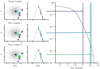 |
Fig. 1. Overview of the likelihood-ratio test analysis used in IC18. The left column shows a reconstructed neutrino direction and its angular uncertainty on the sky with a cross and grey contours, respectively. Nearby source directions are shown by the blue circles, with darker and larger markers representing their contribution to the 𝒮 term in Eq. (2). The centre column shows a 1D projection with the bars representing the flux weights, wi, model for each source. The right panel shows the inverse cumulative test statistic distribution in grey, with the test statistics calculated in each case indicated by the arrows. The weights of nearby sources strongly influence the test statistic value and that different scenarios can lead to significant results. |
With this in mind, we model a population of flaring blazars based purely on the available information in γ rays to explore the implications of this result. References to blazars and flares in the text should be understood to mean γ-ray-bright blazars and γ-ray flares, respectively.
3. Simulation
Our analysis is based on an empirical model of the blazar population, the goal of which is to develop a simple framework that captures the important features relevant to assess the implications of the proposed neutrino association. A summary of all parameters introduced in this section, as well as their reference values can be found in Appendices A and B. The code used to implement the simulations can be found in the nu_coincidence repository1. For the blazars we use the popsynth package2 for population synthesis (Burgess & Capel 2021); for the neutrinos we use the icecube_tools package3. For all simulations we assume a baseline joint observation period of IceCube and Fermi of Tobs = 10 years and a flat ΛCDM cosmology with H0 = 67.7 km s−1 Mpc−1, Ωm = 0.307 and ΩΛ = 1 − Ωm = 0.693 (Planck Collaboration XIII 2016).
3.1. Blazar population
There are two main categories of blazars, based on measurements of their optical spectra: Flat-spectrum radio quasars (FSRQs) with strong emission lines and BL Lacertae-like objects (BL Lacs) with only weak emission lines or featureless spectra (Urry & Padovani 1995). The blazar TXS 0506+056 was first classified as a BL Lac, but upon closer investigation it has been flagged as a likely ‘masquerading BL Lac’, so intrinsically an FSRQ, but with hidden emission lines (Padovani et al. 2019). In this way, we study both FSRQ and BL Lac populations here.
We consider the density of sources as a function of the rest frame γ-ray luminosity in the 0.1–100 GeV range, Lγ, the redshift, z, and the spectral index, Γ, such that
 (8)
(8)
where fL(Lγ) is the luminosity function, fΓ(Γ) is the distribution of spectral indices, dN/dV is the source density per comoving volume and dV/dz is the comoving volume element (see e.g., Peacock 2010). We assume that fL(Lγ) does not evolve, similar to the ‘pure density evolution’ models presented in Ajello et al. (2012, 2014). This choice is motivated by the best-fit model found in Marcotulli et al. (2020). Our results are also robust to the possibility of an evolving luminosity function, as shown in Appendix C.
For both FSRQs and BL Lacs, we model the luminosity function as a broken power law
 (9)
(9)
Here, Lbr is the break luminosity and CL is defined such that f(Lγ) is normalised between Lγ, min and Lγ, max. The spectra of these sources is assumed to be well-described by a power-law with a single spectral index. For both populations, we use a normal distribution model for the spectral index distribution
 (10)
(10)
where μΓ and σΓ are the mean and standard deviation, respectively. Based on the results of Ajello et al. (2012, 2014), we use different parametrisations for FSRQs and BL Lacs. For FSRQs
 (11)
(11)
where ρ0 is the local source density at z = 0 and the other parameters give the shape of the distribution (Cole et al. 2001). For BL Lacs, we simply use
 (12)
(12)
Using this parametrisation, the total number of blazars is independent of the luminosity and spectral index as these are normalised to integrate to one. Therefore, the expected total number of objects in the observable Universe is given by
 (13)
(13)
The ability of the Fermi-LAT to detect an individual blazar depends on its luminosity, distance and spectral index. The Fermi-LAT instrument is sensitive down to some minimum flux and sources with harder spectra can be detected down to lower fluxes (Abdo et al. 2010). In this work, we implement this effect as a cut on the energy flux of an object such that the probability of detection is modelled as
 (14)
(14)
where  , and a and b describe the linear boundary. This selection is made on the observed values of Fγ and Γ, including the observational uncertainties. The true values of Fγ and Γ could fall below this boundary.
We choose a reference set of parameters reflecting the best-fit models of Ajello et al. (2012, 2014) that also gives a γ-ray detected blazar population that is consistent with the results reported in the Fermi 4FGL (Abdollahi et al. 2020) and 4LAC (Ajello et al. 2020) catalogues (see Appendix A for details). We include unclassified blazars in our modelling, assuming for the reference case that 90% of unclassified blazars are actually BL Lacs, and the rest are FSRQs. Later in Sect. 4, we also consider alternative cases where we completely disregard unclassified blazars, or assume that their classification follows the ratio of detected BL Lacs and FSRQs.
Motivated by the difficulty in estimating the properties of the unknown blazar populations, we also consider two extreme cases of our BL Lac and FSRQ population models that lead to lower and higher numbers of detected sources, within reasonable bounds (± ∼ 50% of the reference value). The luminosity function and density evolution for these models are shown in Fig. 2. The distributions of blazar properties for an example simulation under the reference model are also shown in Fig. 3.
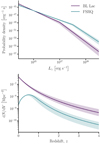 |
Fig. 2. Luminosity function (upper panel) and the source density evolution (lower panel) are shown for the range of blazar population models tested. The reference models are shown by solid curves, and the shaded regions indicate the bounds of the extreme models. The density evolution can be compared to Fig. 11 in Ajello et al. (2014), although their results are for a ‘luminosity-dependent density evolution’, and so should not be expected to be exactly the same as our simpler model. |
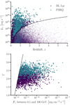 |
Fig. 3. Distributions of blazar properties for an example simulated blazar population assuming the reference model. The upper panel shows Lγ and z and the lower panel shows Γ and Fγ (cf., Fig. 4 in Ajello et al. 2020). In both cases, the dashed lines show the implemented selection. In the upper panel, non-observed blazars are also shown with transparent points. In this particular simulation, there are a total of 17 551 sources, of which 2988 are detected (2206 BL Lacs and 782 FSRQs). |
3.2. Blazar flares
To model the flaring behaviour of blazars, we use an empirical model that is based on the results of the Fermi all-sky variability analysis (FAVA, Abdollahi et al. 2017). FAVA is a photometric analysis of the Fermi-LAT data that searches for flux variations with a time resolution of one week. The search is carried out over two energy bands, from 0.1–0.8 GeV to 0.8–300 GeV. If deviations of > 6σ in one energy band or > 4σ in both energy bands with respect to the average are found, then the flares are catalogued. The results are updated in real-time, and the FAVA analysis of TXS 0506+056 is one of the ways in which it was identified as an active source.
We use the second FAVA catalogue with 7.5 years of data (Abdollahi et al. 2017) as a basis for modelling the fraction of variable blazars in a population, as well as the rate, duration and amplitude of significant γ-ray flares. The choice of power-law distributions is motivated by the observed values and the same parametrisation is used for both BL Lacs and FSRQs. Blazar variability is seen to be luminosity dependent, with more luminous (Lγ ≳ 1046 erg s−1) objects tending to be more variable, although this is partly due to detection effects (Ackermann et al. 2011). We do not model this directly here, but instead use different parameters to model the FSRQs as more variable, resulting in a similar effect as FSRQs tend to be brighter (see Figs. 2 and 3).
All sources in a given population have a probability to exhibit variable behaviour, which we parametrise with the expected fraction of variable sources, fvar. Sources that are not variable have a flare rate of Rf = 0. The distribution of flare rates for variable sources is given by a bounded power law distribution
 (15)
(15)
for  . Here CR is defined such that the distribution is normalised. The flare rate can then be used to calculate the expected number of flares,
  , in a given observation period, Tobs. Flares are assumed to occur uniformly in time over the specified Tobs. Each flare has a duration, τ, that is also distributed according to a bounded power law
 (16)
(16)
where Cτ is again defined to normalise the distribution. The bounds, τmin and τmax, are set in such a way as to ensure a minimum duration of one week and a maximum duration that does not result in overlapping flares. Finally, each flare also has an amplitude, Af, defined as the multiplicative factor by which the luminosity is temporarily increased for the flare duration. As we consider only large flares here, such as would be counted as significant by a FAVA analysis, we model the distribution of amplitudes as a Pareto distribution
 (17)
(17)
where  is the minimum amplitude and ηA > 0 is the index.
This flare model is obviously a simplification of the complexity present in actual blazar lightcurves, with variability seen over a wide range of timescales (see Böttcher 2019 for a recent review). Ideally, we would start from a physically motivated model that describes such variable emission as a function of the blazar properties, which could be convolved with the blazar number density to calculate the expected resulting contribution as a function of time. However, in IC18, blazar lightcurves are binned into intervals of one month when comparing with the time of neutrino emission, so we choose a more discrete flare model to reflect this. Given the typical timescale of a few months for flare durations, our ‘on/off’ description of blazar flares is a reasonable choice. We note that by averaging over long periods, short spikes in the emission that are easier to detect due to lower instantaneous background rates are not modelled and the resulting flux is generally harder to detect. This choice4 could have an impact on the results presented in Sect. 3.3.
3.3. The blazar–neutrino connection
To examine the case of a possible blazar-neutrino connection, in this work we consider two distinct approaches to modelling the neutrino emission. Firstly, we consider no connection between the blazar population and the observed high-energy neutrino flux. In this case, the neutrino emission is modelled as an isotropic, diffuse flux incident at the Earth, at a level consistent with the results of IceCube observations. This ‘null model’ allows us to evaluate the probability for chance coincidences to be present in this scenario, as detailed further in Sect. 4.
We also consider a direct connection between the γ-ray and neutrino emission, motivated by that assumed in IC18 to arrive at the 3σ result, as discussed in Sect. 2. In particular, we assume that the energy flux in neutrinos is some factor of that in gamma rays such that
 (18)
(18)
where Fν is defined as the integral of the flux between 10 TeV and 100 PeV, and Fγ is defined similarly between 1 and 100 GeV. Blazars in the population then continuously produce neutrinos according to Eq. (18), and their emission is amplified suitably during flaring periods. This ‘connected model’ is used to examine the implications of an assumed blazar–neutrino connection for the blazar population in Sect. 5.
By adopting the relation stated in Eq. (18), we assume that Yνγ is the same for all blazars. This is not physically motivated, as we would expect that the ability of a blazar to produce neutrinos would depend on its physical properties (e.g., proton content and energies) that one expects to vary from source to source. Moreover, a connection between the GeV photon flux and the TeV neutrino flux might not be universally motivated by physical assumptions. In single-zone hybrid leptohadronic scenarios for TXS 0506+056 (Keivani et al. 2018; Gao et al. 2019; Cerruti et al. 2019; Gasparyan et al. 2022), the GeV photon flux primarily results from synchrotron self-Compton of the lower-energy synchrotron component. Thus, the flux scales proportional to the product of the number of electrons (ne) and low-energy photons (nγ). On the other hand, the flux of high-energy neutrinos results from the interaction of accelerated protons with the same low-energy synchrotron photons; therefore, roughly scaling as the product of the number of protons (np) and nγ. This implies that  . In summary, the observed flux in GeV photons and TeV neutrinos might not be due to the same underlying processes, as possible contributions to the GeV photon flux from hadronic processes could be dominated by those from purely leptonic processes. Additionally, there is no reason to believe that Yνγ remains constant across a population of flares or even within a single outburst. For proton-synchrotron models, the GeV photon flux scales proportional to np while the TeV neutrino flux again scales proportional to the product of np and the low-energy nγ. Therefore, Yνγ ∝ nγ which again should vary from source to source and within a single outburst. Thus, although Yνγ could be useful as an observational tool, it is not a well-motivated quantity for forward simulation. Nevertheless, the weighting of the likelihood used in IC18 implicitly makes the assumption shown in Eq. (18), as detailed in Sect. 2, and so we investigate its implications here.
Another unphysical assumption in the likelihood that we detailed in Sect. 2 is that the neutrinos are always produced with a power-law spectrum that has a fixed spectral index. In most physical scenarios appropriate for blazar flare emission, the peak and spectral index of the neutrino spectrum are determined by the distribution of low-energy photons. Notably, this results in a hard spectrum of E−0.3 (Padovani et al. 2015; Gasparyan et al. 2022), very different to the assumption of E−2.13 used here (motivated by the assumptions of IC18). These caveats should caution the reader that the limits on Yνγ presented in Sect. 5 should be interpreted in the context of the original likelihood assumptions and not that of a full physical model.
3.4. Neutrino observations
The IceCube neutrino observatory reconstructs the energy and direction of incoming neutrinos from secondary Cherenkov radiation signals (Aartsen et al. 2017d). An important background to the study of astrophysical neutrinos is the contribution of atmospheric neutrinos, produced via cosmic ray interactions in the Earth’s atmosphere. IceCube has set up a real-time alerts system with the goal of using multi-messenger observations to help identify possible neutrino sources through follow-up programmes (Aartsen et al. 2017c). To optimise the potential of this system, published alert events are selected via cuts on the amount of photons deposited in the detector, and to favour track-like event topologies from the charged-current interactions of muon neutrinos. This results in the selection of events with a reasonable likelihood of being astrophysical and smaller angular errors on the reconstructed directions. These alerts come in two main categories: the high-energy starting tracks (HESE); and the extremely high-energy tracks (EHE). This real-time alert system led to the identification of IC170922A reported in IC18.
In this work, we model the detection of neutrino alerts to connect with the analysis carried out in IC18. We make use of publicly available information on the effective area of IceCube together with sensible cuts on the reconstructed deposited energy to build our detector model, further details are given in Appendix B. Since June 2019, the alerts system has been updated from the HESE/EHE selections to the new and improved astrotrack bronze and gold selections reported in Blaufuss et al. (2019). For the sake of relevance to IC18, we only consider the HESE and EHE alerts in our analysis.
For the diffuse neutrino emission simulated in the null-model case, we model the per-flavour astrophysical neutrino flux as a power law with a flux normalisation of 2 × 10⁻¹⁸ GeV−1 cm−2 s−1 sr−1 and a spectral index of 2.6. The atmospheric component is modelled similarly with a flux normalisation of 5 × 10⁻¹⁸ GeV−1 cm−2 s−1 sr−1 and a power-law index of 3.7 (reasonable for the energies of > 10 TeV considered here). These choices are based on those assumed in Aartsen et al. (2017c) and Kopper et al. (2016), to reproduce the expected number of atmospheric and astrophysical alerts each year. Further information is given in Appendix B.
4. Chance coincidences
We first consider the case where there is no connection between blazars and neutrinos, as described by the null model introduced in Sect. 3.3. The goal of simulating this case is to understand the level of chance coincidences between blazars and neutrinos that can occur, even if they are actually unrelated. As described in Sect. 3, we generate random sets of blazar populations and neutrino observations. For each simulated survey, we count the number of coincident detections. Repeating this procedure ∼104 times, we report the fraction of surveys which satisfy various coincidence checks, which is effectively the probability of such a search resulting in a false positive.
To show how the number of chance coincidences changes for different searches, we consider different coincidence criteria. We first define spatial coincidence as a blazar position being inside the 90% confidence region of a detected neutrino event, and temporal coincidence as a neutrino arrival time being during the flaring period of a detected blazar. We then consider three levels of coincidence: Spatial coincidence of neutrinos with blazars (spatial), spatial coincidence of neutrinos with variable blazars (spatial + variable), and spatial and temporal coincidence of neutrinos with blazar flares (spatial + variable + flare).
For the reference blazar model parameters given in Appendix A, the distributions of the number of coincidences are shown in Fig. 4. We see that while BL Lacs tend to have a larger number of spatial coincidences as they are more numerous, FSRQs have more variable coincidences as they flare more often. In general, we can expect observations of up to around 32 spatial blazar coincidences and 8 variable blazar coincidences to be consistent with the null model. Flare coincidences are rare, but not completely unexpected. We find that 2.0% and 5.6% of BL Lac and FSRQ surveys of this size, respectively, result in at least one flare coincidence. This gives a total chance coincidence probability for flaring blazars and neutrino alerts of 7.6%. The result is not affected much if we consider the number of surveys leading to exactly one flare coincidence, reducing to 7.4% in this case.
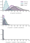 |
Fig. 4. Distributions of the number of coincidences for simulations of the reference model given in Appendix A. Three difference coincidence levels are shown, as explained in the text. The BL Lac and FSRQ survey results are shown in purple and blue, respectively, with the total combined blazar survey shown in black. |
Roughly half of these flare coincidences will actually be due to the atmospheric neutrino background, which contributes 4.5% to the total 7.6% for the reference model case discussed above. For neutrino events with energies in the range 200 TeV–7.5 PeV, the 90% confidence interval found for IC170922A, (see Fig. S2 in IC18), ∼37% are due to the atmospheric background.
Considering the higher and lower source density models that were introduced in Sect. 3.1, the chance coincidence probabilities decrease and increase as expected relative to the number of detected sources present in the simulation. For brevity, we focus here on the interesting case of spatial + variable + flare coincidences, most relevant to the results of IC18. The chance coincidence probability for these flare coincidences for the different population models is shown in Fig. 5. Even considering rather large changes in the population, we see that the total chance coincidence probability is between 3.8% and 12.7%, with FSRQs as the dominant contribution to this value.
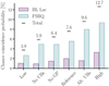 |
Fig. 5. Chance coincidence probability of flare coincidences for the range of blazar population models shown in Fig. 2 and other variations described in the text. For each case, the separate contributions of BL Lacs and FSRQs are shown in purple and blue, respectively. |
To check the robustness of these results, we also consider further variations to our reference blazar population model. We test excluding 10° either side of the Galactic plane in the selection of detected blazars (No GP), motivated by the 4LAC catalogue results. Additionally, we consider different treatment of the unclassified blazars (UBs) reported in the Fermi surveys. For our reference model, we assume that most (90%) of all unclassified blazars are BL Lacs. We also consider excluding unclassified blazars completely (No UBs) or assuming that the ratio of FSRQs to BL Lacs is the same as for classified blazars (Alt. UBs). The impact of these assumptions is also shown in Fig. 5. Changing the diffuse neutrino flux model also has a minor impact on the results and this is detailed in Appendix B.
The expected value of spatial coincidences is typically less than that seen in current searches, with 26 Fermi-detected blazar sources (15 BL Lacs, six FSRQs, and five unclassified blazars) found within the 90% error region of IceCube alert events (Giommi et al. 2020)5. For a fair comparison with the assumptions used in Giommi et al. (2020), we must consider the number of spatial coincidences for the No GP case introduced above, as shown in Fig. 6. We find that the currently observed number of spatial coincidences is more than the most probable value, but consistent with the expectations of the null model. In our null simulation we are most likely to see 14 coincidences, with a probability of 0.08, and the probability of seeing 26 coincidences is 0.016. This result is consistent with the conclusions of Giommi et al. (2020), as their most significant result is calculated considering the intermediate and high energy peaked BL Lac sub populations and neutrino event error regions that are enlarged by a factor of 1.3 to account for possible underestimation, neither of which are considered here.
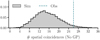 |
Fig. 6. Distribution of the number of spatial coincidences found for the No GP case (histogram), to allow comparison with the observed number of 26 spatial coincidences reported in Giommi et al. (2020; dashed line). |
The chance coincidence probability that we find is small, but non-negligible, and becomes increasingly problematic for longer or deeper surveys. To connect with the p-value of 3σ (i.e., a chance coincidence probability of ∼0.1%) reported in IC18, it is important to remember that their calculation is tied to the model assumed in the likelihood for wi, model(tν) as reviewed in Sect. 2. When assuming no γ-ray–neutrino connection, that is wi, model(tν)=1, IC18 also find a higher chance coincidence probability. Assuming wi, model(tν)=Fγ(tν) or wi, model(tν)=Fγ(tν)/⟨Fγ⟩ is necessary to find a significant association. To illustrate this effect, we set a threshold on Fγ and the flare amplitude required for a coincident detection, and show how our chance coincidence probability changes as a function of this threshold in Fig. 7. Our goal here is not to exactly reproduce the results of IC18, but to consider the possibility of a blazar-neutrino connection from an independent standpoint and compare the results in context.
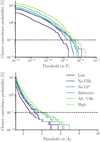 |
Fig. 7. Chance coincidence probability as a function of the blazar flux (upper panel) and flare amplitude (lower panel) threshold. The different coloured lines show the different blazar population model assumptions, as in Fig. 5, and the dashed line at 0.1% gives the ∼3σ level. |
Figure 7 shows that we require a blazar flux ≳10−9–10−8 erg cm−2 s−1 or a flare amplitude threshold ≳3–5 for a chance coincidence probability of < 0.1%. To give these values context, for the reference model around 50 blazars in each survey have Fγ > 10−9 erg cm−2 s−1 and the flux of TXS 0506+056 during the 1 month period around the arrival of IC170922A was 3.3 × 10⁻¹⁰ erg cm−2 s−1 (IC18). Similarly, about 50 flares in each survey have A > 3 and the corresponding amplitude of the TXS 0506+056 blazar flare over a 6 month period is ∼3.5 (IC18). The flare amplitude threshold is not equivalent to  defined in Sect. 3.2, as it is a cut applied to the simulated survey and not a parameter of the simulation itself.
To allow for a closer comparison with IC18, we also implement the likelihood ratio test described therein and in Sect. 2. For each simulated survey with one or more flare coincidences, we find the test statistic distribution under the assumption of the null hypothesis using 105 simulated neutrino alerts. We then compare the observed test statistic with this null distribution to find the significance. When using a weighting based on a linear relationship with the γ-ray flux, we confirm that we find a chance coincidence probability of ≈0.13% for events with a test statistic threshold corresponding to 3σ. This value is as expected for a one-sided Gaussian definition of the p-value.
5. Implications of a γ-ray–neutrino connection
We now study the case of a connection between the integrated γ-ray emission of blazars and the production of neutrinos, introduced as the connected model in Sect. 3.3. In IC18, Yνγ is estimated to be in the range of 0.5–1.7, assuming a relevant neutrino energy range of 200 TeV–7.5 PeV and depending on the details of the neutrino emission timescale. However, taking Yνγ and naively extrapolating to the whole blazar population, we overshoot both the total number of neutrino alerts and the number of alerts that share common sources (Capel 2021).
This overproduction can be accounted for if we adjust our estimate of the neutrino flux necessary for the observation of a single alert event. We expect that there are other sources which may contribute on a similar level to that of TXS 0506+056. So, the expected contribution from this individual source may be ≪1, but the integrated contribution from all sources in the population could be 𝒪(1), as required for a detection (Strotjohann et al. 2019). Indeed, SED modelling of the multiwavelength spectra of TXS 0506+056 indicate that it is challenging to reach expected event numbers of 𝒪(1) for this particular source, without overshooting the X-ray measurements or invoking multi-zone models (Keivani et al. 2018; Cerruti et al. 2019; Gao et al. 2019; Xue et al. 2019; Liu et al. 2019). Additionally, studies on the modelling of similar blazar flares show expected neutrino event numbers of ≪1 for individual sources (Oikonomou et al. 2019; Palladino et al. 2019; Kreter et al. 2020). With this in mind, we allow for the expected number of neutrino events from TXS 0506+056 to be < 1 and explore the blazar–neutrino connection in this case.
To estimate the constraints on Yνγ implied by the observation of a single neutrino alert from the whole blazar population, we ran ∼104 simulations of our reference blazar model for a range of different Yνγ values. We recorded the fraction satisfying the constraint  , where
  is the detected number of neutrino alerts in IceCube after 10 years of observations. The resulting constraints on Yνγ depend on whether we considered steady-state neutrino emission from blazars or purely flaring emission, as shown in Fig. 8. We see that the constraints are several orders of magnitude stronger when considering contributions from all blazar emission, requiring Yνγ ≲ 10−3. When considering only contributions from blazar flares to the neutrino flux, Yνγ ∼ 10−3–10−1 is consistent with
  . We can also see that this constraint is dominated by the FSRQ population, as expected from the higher observed variability in this case. Lowering the number of sources in the blazar population relaxes these constraints, and vice versa.
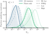 |
Fig. 8. Fraction of simulated surveys satisfying |

We now also consider the more conservative constraints on Yνγ from requiring  , the total number of observed neutrino alert events in 10 years7, as reported in IC18 and the NASA GCN archive8. We also know that we have yet to observe more than two neutrino alerts that are consistent with a shared source direction9. In this way, we also require
  , where
  is the numbers of sources that produce more than one detected neutrino event. The results are shown in Fig. 9. Here, the upper limits are slightly relaxed compared to those shown in Fig. 8, Yνγ is restricted to ≲10−2 when considering all blazar emission and ≲1 when only considering blazar flares.
For all cases considered above, the contribution to neutrino alerts from the undetected blazar population only really becomes relevant at the level of 5–10% when considering all blazar emission, both steady-state and flaring. Practically all neutrino alerts from the flaring population originate in blazars that would also be detected in γ rays. Whilst this is somewhat intuitive given the simplistic connection between γ rays and neutrinos assumed, it is generally important to keep in mind the possible neutrino signal from uncatalogued blazars when considering the implications of observational constraints.
6. Discussion
Using the simulation model described in Sect. 3, we demonstrated in Sect. 4 that the assumption of a γ-ray–neutrino connection is necessary to find a low chance coincidence probability for neutrino alerts and γ-ray flaring blazars. We then explored the constraints on such a connection implied by the blazar population in Sect. 5. These constraints are broadly in agreement with the predictions presented in the framework of the blazar simplified view (Padovani et al. 2015) and the independent constraint of Yνγ ≤ 0.13 from the non-observation of events with deposited energy ≳1 PeV in 7 years of IceCube data (Aartsen et al. 2016b, 2017b). There are also more detailed theoretical investigations of individual blazars, for which the constraints on the hadronic fraction of γ-ray emission are strong (Oikonomou et al. 2019; Palladino et al. 2019; Kreter et al. 2020).
While relevant for the model presented in IC18, the results in Sect. 5 are dependent on the assumptions of our connected γ-ray and neutrino model for blazars. The simplified and unphysical form of this connection does not allow us to interpret the constraints on Yνγ beyond the context of the IceCube likelihood and its implied emission model. Considering a more physical connection, it would be reasonable to assume that Yνγ varies both across the blazar population and during flaring periods, weakening the constraints shown here. Additionally, we would expect that the neutrino emission follows a peaked spectrum that varies between blazars. This expectation will also impact the results compared to the assumption of a fixed E−2.13 power-law neutrino emission for all blazars used here, but the details of this effect will depend on the location of the peak of the neutrino spectrum relative to the TeV–PeV energy range observable by IceCube. Alleviating these issues would require a more physically motivated likelihood and proper joint fitting of neutrino and photon spectra with multi-messenger tools such as 3ML (Vianello et al. 2015) as well as exploring population simulations with physically derived spectral models such as that presented in Gasparyan et al. (2022).
It has been shown that the required target photon field for efficient TeV–PeV neutrino production could lead to sources becoming opaque to γ rays in the 1–100 GeV range due to γγ interactions, and that cascades in the source environment would lead to electromagnetic contributions down to KeV or MeV energies (Dermer et al. 2007; Murase et al. 2016; Reimer et al. 2019; Das et al. 2022). So, we actually expect γ-ray emission in the Fermi-LAT energy range to be suppressed during periods of increased neutrino emission, unless the fundamental understanding of relativistic jets is wrong. In this case, other wavelengths may be more indicative of a possible blazar–neutrino connection, such as radio or X-rays (a review can be found in Giommi & Padovani 2021). In more recent work, a significant correlation between neutrino hotspots in the Southern sky and blazars in the Roma-BZCat catalogue has been reported in Buson et al. (2022), while Liodakis et al. (in prep.) conclude that we should not expect to be able to identify significant correlations between radio flares in AGN and neutrinos with the currently available data and methods.
Given the form of the likelihood described in Sect. 2 and the results presented in IC18, it is clear that assuming no relation to the γ-ray flux, or an inversely proportional relation would not lead to a significant association between IC170922A and TXS 0506+056. While we plan to explore other models in future, the main goal of this work is to study the choices made in the IC18 analysis that led to the 3σ significance for the IC170922A–TXS 0506+056 and their direct implications. As such, we focus on a linearly proportional connection to γ rays.
Several studies have investigated possible correlations of neutrinos with known catalogues of γ-ray blazars using likelihood-based stacking analyses, including weighting the source contribution by Fγ (Aartsen et al. 2017a; Huber 2019; Neronov et al. 2017). The non-observation of significant correlations in the time-integrated data is used to place upper limits on the contribution of these sources to the observed neutrino flux of ∼10–30%, depending on the model assumptions. Futhermore, the blazar contribution has also been limited to ∼6% by an alternative approach considering three proposed individual blazar associations (Bartos et al. 2021). Requiring that the total integrated flux from the population is less than the total observed diffuse neutrino flux leads to similar constraints on Yνγ to those shown in Fig. 9. Applying a full point source search analysis to each simulated neutrino survey would likely yield even stronger constraints on Yνγ, due to the inclusion of information lower-energy events, but this approach was not tested here.
The IceCube Collaboration has also found a flare of lower energy neutrinos at the 3.5σ significance level by looking into the past data at the position of TXS 0506+056 (Ice Cube Collaboration 2018c). We do not focus on this result in our work, as the analysis is conditioned on the assumption that the IC170922A–TXS 0506+056 association is real in order to select this position in the sky. The low-energy neutrino flare was found during a period where TXS 0506+056 was not in a γ-ray flaring state, despite the fact that a γ-ray–neutrino connection is required for the original high-energy neutrino association to be significant. To avoid the logical inconsistency between the two analyses, we focus on studying the IC170922A–TXS 0506+056 association and its implications in isolation here.
7. Conclusions
We present a framework for studying the implications of co-incident multi-messenger detections using Monte Carlo simulations. Our approach allows us to connect individual coincidences to the relevant source populations and model assumptions. We applied this framework to the case of a coincident high-energy neutrino and γ-ray flaring blazar reported in IC18.
Assuming no connection between blazars and neutrinos, we find that there is a 7.6% chance of mistakenly finding high-energy neutrino alerts that are coincident with γ-ray blazar flares in 10-year surveys. This value ranges from 3.8% to 12.7% when considering extreme cases of our blazar population model. To reduce this chance to the level where an IC170922A–TXS 0506+056-like event has a 3σ significance (i.e., ∼0.1%), we must also consider the blazar flux or flare amplitude at the time of the neutrino event, similar to the likelihood weighting used in IC18 and reviewed in Sect. 2. We also show that we expect to see as many as ∼32 directional blazar–neutrino chance coincidences in a 10-year survey and we verified that this value is consistent with current observations.
Considering that a linearly proportional γ-ray–neutrino flux connection is required for the IC170922A–TXS 0506+056 to be statistically significant, we then explored the implications of this assumption for the blazar population as a whole. We find that either the γ-ray–neutrino connection is restricted to Yνγ ≲ 10−2, or that only a small fraction of blazars contribute to the neutrino flux. However, in Capel et al. (2020), we demonstrate that rare and luminous blazars capable of fulfilling these scenarios are also strongly constrained by the non-observation of point sources, further complicating the physical picture (consistent with Yuan et al. 2020). Alternatively, if we only consider contributions from blazar flares, we expect Yνγ ∼ 10−3–10−1 to be consistent with one neutrino–blazar flare coincidence in 10 years of observations. The constraints on Yνγ should be interpreted in the context of the likelihood model assumed in IC18 and described in Sect. 2, rather than that of a more detailed physical model.
The simplified nature of the models for neutrino association that are built into the likelihoods used in IC18 and other IceCube point source searches mean that finding an object with a rare property that lies within a neutrino error region can lead to a significant result. When interpreting such a result, it is important to understand if the rare property is physically well-motivated. Here, we explore the implications of the model assumed in IC18 for a population of blazars and find that the expected neutrino signals are overproduced with respect to observations, unless small values of Yνγ are considered, or only blazar flares contribute to neutrino emission. Both of these results motivate changes to the original likelihood used: If Yνγ is very small, the γ-ray flux is likely not the most useful weight to use. If only blazar flares contribute, non-flaring sources should not be considered. In future, the use of more physical, interpretable models in association analyses can help to resolve this confusion.
In the future, our approach can be used to study similar multi-messenger detections, inform the logical consistency of likelihood models used in such searches and aid in the design of targeted follow-up programmes. By defining a detailed generative model that connects source populations to neutrino observations, we also lay the foundation for performing inference of population parameters from observations in this setting.
8. Software
NumPy (Harris et al. 2020), SciPy (Virtanen et al. 2020), Astropy (Astropy Collaboration 2013, 2018), Matplotlib (Hunter 2007), h5py (Collette 2013), Joblib (Joblib Development Team 2021), popsynth (Burgess & Capel 2021).
We did consider using a more sophisticated model such as damped random walks or structure functions (Kozłowski 2016), but we would in any case attempt to tune these models to reproduce the FAVA results as a baseline.
We consider sources that are present in the Fermi 4FGL catalogue and have a classification of either BL Lac, FSRQ or unclassified blazar. If we include all sources reported in Giommi et al. (2020), the total is 29.
If we consider 29 observed events, this probability becomes 0.004.
Based on the publicly available information, there are a total of 67 HESE/EHE alerts up until mid-2019, when the new system was introduced. Here we assume 70 events for the 2010–2020 period, but using 67 has negligible effect on Fig. 9.


In the public HESE events, there are two events with larger angular uncertainties that are consistent with a shared source location.
Acknowledgments
We thank the Max Planck Computing and Data Facility for the use of the Raven HPC system. F. Capel acknowledges financial support from the Excellence Cluster ORIGINS, which is funded by the Deutsche Forschungsgemeinschaft (DFG, German Research Foundation) under Germany’s Excellence Strategy – EXC-2094-390783311. J. M. Burgess acknowledges financial support by the Deutsche Forschungsgemeinschaft (SFB 1258). We thank Damien Bégué for useful conversations on the physics of neutrino production.
References
- Aartsen, M. G., Abbasi, R., Abdou, Y., et al. 2013, Science, 342, 1242856 [Google Scholar]
- Aartsen, M. G., Abraham, K., Ackermann, M., et al. 2015, Phys. Rev. Lett., 115, 96 [CrossRef] [Google Scholar]
- Aartsen, M. G., Abraham, K., Ackermann, M., et al. 2016a, ApJ, 833, 18 [NASA ADS] [CrossRef] [Google Scholar]
- Aartsen, M. G., Abraham, K., Ackermann, M., et al. 2016b, Phys. Rev. Lett., 117, 241101 [CrossRef] [Google Scholar]
- Aartsen, M. G., Abraham, K., Ackermann, M., et al. 2017a, ApJ, 835, 45 [Google Scholar]
- Aartsen, M. G., Abraham, K., Ackermann, M., et al. 2017b, Phys. Rev. Lett., 119, 259902 [CrossRef] [Google Scholar]
- Aartsen, M. G., Ackermann, M., Adams, J., et al. 2017c, Astropart. Phys., 92, 30 [Google Scholar]
- Aartsen, M. G., Ackermann, M., Adams, J., et al. 2017d, J. Instrum., 12, 03012 [Google Scholar]
- Abbasi, R., Ackermann, M., Adams, J., et al. 2022, ApJ, 928, 50 [NASA ADS] [CrossRef] [Google Scholar]
- Abbott, B. P., Abbott, R., Abbott, T. D., et al. 2017, ApJ, 848, L13 [CrossRef] [Google Scholar]
- Abdo, A. A., Ackermann, M., Ajello, M., et al. 2010, ApJ, 720, 435 [NASA ADS] [CrossRef] [Google Scholar]
- Abdollahi, S., Ackermann, M., Ajello, M., et al. 2017, ApJS, 846, 34 [NASA ADS] [Google Scholar]
- Abdollahi, S., Acero, F., Ackermann, M., et al. 2020, ApJS, 247, 33 [Google Scholar]
- Ackermann, M., Ajello, M., Allafort, A., et al. 2011, ApJ, 743, 171 [Google Scholar]
- Ajello, M., Shaw, M. S., Romani, R. W., et al. 2012, ApJ, 751, 108 [NASA ADS] [CrossRef] [Google Scholar]
- Ajello, M., Romani, R. W., Gasparrini, D., et al. 2014, ApJ, 780, 73 [Google Scholar]
- Ajello, M., Angioni, R., Axelsson, M., et al. 2020, ApJ, 892, 105 [NASA ADS] [CrossRef] [Google Scholar]
- Ajello, M., Atwood, W. B., Axelsson, M., et al. 2021, Nat. Astron., 5, 385 [CrossRef] [Google Scholar]
- Ashton, G., Burns, E., Canton, T. D., et al. 2018, ApJ, 860, 6 [NASA ADS] [CrossRef] [Google Scholar]
- Astropy Collaboration (Robitaille, T. P., et al.) 2013, A&A, 558, A33 [NASA ADS] [CrossRef] [EDP Sciences] [Google Scholar]
- Astropy Collaboration (Price-Whelan, A. M., et al.) 2018, AJ, 156, 123 [Google Scholar]
- Bartos, I., Veske, D., Keivani, A., et al. 2019, Phys. Rev. D, 100, 083017 [NASA ADS] [CrossRef] [Google Scholar]
- Bartos, I., Veske, D., Kowalski, M., Márka, Z., & Márka, S. 2021, ApJ, 921, 45 [NASA ADS] [CrossRef] [Google Scholar]
- Blaufuss, E., Kintscher, T., Lu, L., & Tung, C. F. 2019, Proc. ICRC, 1021 [Google Scholar]
- Böttcher, M. 2019, Galaxies, 7, 20 [Google Scholar]
- Burgess, J., & Capel, F. 2021, J. Open Source Softw., 6, 3257 [NASA ADS] [CrossRef] [Google Scholar]
- Buson, S., Tramacere, A., Pfeiffer, L., et al. 2022, ApJ, 933, L43 [NASA ADS] [CrossRef] [Google Scholar]
- Capel, F. 2021, Proc. ICRC, 981 [Google Scholar]
- Capel, F., & Mortlock, D. J. 2019, MNRAS, 484, 2324 [NASA ADS] [CrossRef] [Google Scholar]
- Capel, F., Mortlock, D. J., & Finley, C. 2020, Phys. Rev. D, 101, 123017 [NASA ADS] [CrossRef] [Google Scholar]
- Cerruti, M., Zech, A., Boisson, C., et al. 2019, MNRAS, 483, L12 [NASA ADS] [CrossRef] [Google Scholar]
- Cole, S., Norberg, P., & Baugh, C. M. 2001, MNRAS, 326, 255 [NASA ADS] [CrossRef] [Google Scholar]
- Collette, A. 2013, Python and HDF5 (California: O’Reilly) [Google Scholar]
- Das, S., Gupta, N., & Razzaque, S. 2022, Implications of Multiwavelength Spectrum on Cosmic-ray Acceleration in Blazar TXS 0506+056 [Google Scholar]
- Dermer, C. D., Ramirez-Ruiz, E., & Le, T. 2007, ApJ, 664, L67 [NASA ADS] [CrossRef] [Google Scholar]
- Franckowiak, A., Garrappa, S., Paliya, V., et al. 2020, ApJ, 893, 162 [Google Scholar]
- Gao, S., Fedynitch, A., Winter, W., & Pohl, M. 2019, Nat. Astron., 3, 88 [NASA ADS] [CrossRef] [Google Scholar]
- Gasparyan, S., Bégué, D., & Sahakyan, N. 2022, MNRAS, 509, 2102 [Google Scholar]
- Giommi, P., & Padovani, P. 2021, Universe, 7, 492 [NASA ADS] [CrossRef] [Google Scholar]
- Giommi, P., Glauch, T., Padovani, P., et al. 2020, MNRAS, 497, 865 [Google Scholar]
- Graham, M. J., Ford, K. E. S., McKernan, B., et al. 2020, Phys. Rev. Lett., 124, 251102 [NASA ADS] [CrossRef] [Google Scholar]
- Harris, C. R., Millman, K. J., van der Walt, S. J., et al. 2020, Nature, 585, 357 [NASA ADS] [CrossRef] [Google Scholar]
- Huber, M. 2019, Proc. ICRC, 2019(358), 917 [Google Scholar]
- Hunter, J. D. 2007, Comput. Sci. Eng., 9, 90 [NASA ADS] [CrossRef] [Google Scholar]
- Ice Cube Collaboration 2018a, All-sky Point-source IceCube Data Years 2010-2012, online [Google Scholar]
- Ice Cube Collaboration 2018b, IceCube Catalog of Alert Events up Through Icecube-170922A, online [Google Scholar]
- Ice Cube Collaboration 2018c, Science, 825, eaat2890 [Google Scholar]
- Ice Cube Collaboration (Aartsen, M. G., et al.) 2018d, Science, 361, eaat1378 [NASA ADS] [Google Scholar]
- Joblib Development Team 2021, Joblib: Running Python Functions as Pipeline Jobs [Google Scholar]
- Kadler, M., Krauß, F., Mannheim, K., et al. 2016, Nat. Phys., 12, 807 [Google Scholar]
- Keivani, A., Murase, K., Petropoulou, M., et al. 2018, ApJ, 864, 84 [Google Scholar]
- Kopper, C., Giang, W., & Kurahashi, N. 2016, Proceedings of The 34th International Cosmic Ray Conference - PoS(ICRC2015), 1081 [CrossRef] [Google Scholar]
- Kozłowski, S. 2016, ApJ, 826, 118 [CrossRef] [Google Scholar]
- Kreter, M., Kadler, M., Krauß, F., et al. 2020, ApJ, 902, 133 [Google Scholar]
- Liu, R.-Y., Wang, K., Xue, R., et al. 2019, Phys. Rev. D, 99, 063008 [NASA ADS] [CrossRef] [Google Scholar]
- Marcotulli, L., Mauro, M. D., & Ajello, M. 2020, ApJ, 896, 6 [NASA ADS] [CrossRef] [Google Scholar]
- Murase, K., & Waxman, E. 2016, Phys. Rev. D, 94, 103006 [NASA ADS] [CrossRef] [Google Scholar]
- Murase, K., Guetta, D., & Ahlers, M. 2016, Phys. Rev. Lett., 116, 071101 [NASA ADS] [CrossRef] [Google Scholar]
- Neronov, A., & Semikoz, D. 2020, J. Exp. Theoret. Phys., 131, 265 [NASA ADS] [CrossRef] [Google Scholar]
- Neronov, A., Semikoz, D. V., & Ptitsyna, K. 2017, A&A, 603, A135 [NASA ADS] [CrossRef] [EDP Sciences] [Google Scholar]
- Oikonomou, F., Murase, K., Padovani, P., Resconi, E., & Mészáros, P. 2019, MNRAS, 489, 4347 [Google Scholar]
- Padovani, P., Petropoulou, M., Giommi, P., & Resconi, E. 2015, MNRAS, 452, 1877 [NASA ADS] [CrossRef] [Google Scholar]
- Padovani, P., Oikonomou, F., Petropoulou, M., Giommi, P., & Resconi, E. 2019, MNRAS, 484, L104 [NASA ADS] [CrossRef] [Google Scholar]
- Palladino, A., Rodrigues, X., Gao, S., & Winter, W. 2019, ApJ, 871, 41 [NASA ADS] [CrossRef] [Google Scholar]
- Peacock, J. A. 2010, Cosmological Physics (Cambridge: Cambridge University Press), 89 [Google Scholar]
- Planck Collaboration XIII. 2016, A&A, 594, A13 [NASA ADS] [CrossRef] [EDP Sciences] [Google Scholar]
- Reimer, A., Böttcher, M., & Buson, S. 2019, ApJ, 881, 46 [Google Scholar]
- Strotjohann, N. L., Kowalski, M., & Franckowiak, A. 2019, A&A, 622, L9 [NASA ADS] [CrossRef] [EDP Sciences] [Google Scholar]
- Urry, C. M., & Padovani, P. 1995, PASP, 107, 803 [NASA ADS] [CrossRef] [Google Scholar]
- Veske, D., Márka, Z., Bartos, I., & Márka, S. 2021, ApJ, 908, 216 [NASA ADS] [CrossRef] [Google Scholar]
- Vianello, G., Lauer, R. J., Younk, P., et al. 2015, ArXiv e-prints [arXiv:1507.08343] [Google Scholar]
- Virtanen, P., Gommers, R., Oliphant, T. E., et al. 2020, Nat. Methods, 17, 261 [Google Scholar]
- Xue, R., Liu, R.-Y., Petropoulou, M., et al. 2019, ApJ, 886, 23 [NASA ADS] [CrossRef] [Google Scholar]
- Yuan, C., Murase, K., & Mészáros, P. 2020, ApJ, 890, 25 [NASA ADS] [CrossRef] [Google Scholar]
Appendix A: Blazar model parameters
In Table A.1 we list in full the values for the reference BL Lac and FSRQ populations used in this work, based on the parametrisation introduced in Sect. 3. These parameters were chosen by starting with an equivalent density evolution to that found in Ajello et al. (2012, 2014), and comparing the results of simulations to the 4FGL (Abdollahi et al. 2020), 4LAC (Ajello et al. 2020), and FAVA (Abdollahi et al. 2017) catalogues. The parameters were then tuned to find a reasonable match for the number of detected sources, the number of flaring sources, and the total number of flares, along with the distributions of all observed properties.
Reference blazar model parameters.
We also modelled the detection uncertainties where relevant. For Fγ, these uncertainties follow a log normal distribution centred on the latent value, and with a standard deviation of 0.1, and similarly for Γ we used a normal distribution with standard deviation of 0.1. These choices are based on the values reported in Abdollahi et al. (2020).
To study the impact of our assumptions, we considered variations to this blazar reference model, as detailed in Sects. 3.1 and 4. While we do not reproduce an exhaustive list of parameter values here, all choices are supplied as YAML configuration files in the nu_coincidence repository that can easily be loaded into the main code for reproducibility of the results.
Appendix B: IceCube real-time alerts model
We modelled the diffuse neutrino flux as described in Sect. 3.4 and shown in Fig. B.1. The ratio of the atmospheric and astrophysical factors is the driving factor behind the classification of alert events, and we see that higher energy events are more likely to be of astrophysical than atmospheric origin. The characterisation of the astrophysical flux is still uncertain (see e.g. Fig. 5 in Abbasi et al. 2022). To investigate the effect of this uncertainty, we also considered two extreme cases, as shown by the shaded region in Fig. B.1. These extreme cases describe harder and softer flux models, the details of which are given in Table B.1. The uncertainties on the atmospheric component are considered to be negligible in comparison to those of the astrophysical component. In Table B.1, we also give the chance coincidence probabilities for spatial + variable + flare coincidences, as studied in Sect. 4.
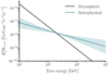 |
Fig. B.1. Per-flavour diffuse neutrino flux used is shown for both the atmospheric and astrophysical components. For the astrophysical case, the two extreme cases also considered bound the shaded region. |
 |
Fig. B.2. Details of the neutrino alert simulations. Left panel: Whole-sky effective area for the HESE and EHE track alerts generated via simulations using the detector mode described in Sect. 3.4. Right panel: Cumulative distribution for the angular resolution of simulated alert events (c.f. Figs. 7 and 9 in Aartsen et al. 2017c). |
Summary of the per-flavour diffuse neutrino flux models considered.
To model the HESE alerts, we used the effective areas from the public dataset associated with Aartsen et al. (2013), summed over all flavours. Similarly, for the EHE alerts, we used the effective areas from Ice Cube Collaboration (2018a) for muon neutrino track events. In both cases, we reduced the effective areas slightly to account for the more stringent event cuts described in Aartsen et al. (2017c), and we modelled the energy resolution using information from the data release associated with Aartsen et al. (2015). For the EHE case, we placed a cut on the reconstructed energies of Ereco > 250 TeV to match the requirements of the alerts stream. For the angular resolution, we again made use of the Ice Cube Collaboration (2018a) dataset, but with small adjustments made such that the resulting 90% confidence regions match what is expected based on Aartsen et al. (2017c) and Ice Cube Collaboration (2018b). Fig. B.2 shows the HESE and EHE effective areas. To find the effective area, we ran simulations of 106 HESE and EHE events from a known power-law spectrum using the setup described in Sect. 3.4. Fig. B.2 shows the cumulative distribution of the angular resolution for HESE and EHE events.
Appendix C: Luminosity-dependent density evolution
Ajello et al. (2012, 2014) find that a luminosity-dependent density evolution (LDDE) best describes the BL Lac and FSRQ luminosity functions. As described in Sect 3.1, we use a simple pure density evolution (PDE) model, motivated by the more recent results of Marcotulli et al. (2020) for all blazars. As the evolution is an important factor in exploring the connection between blazar populations and neutrinos (see e.g. Neronov & Semikoz 2020; Yuan et al. 2020; Capel et al. 2020), we describe the differences in these models and their impact on our conclusions here.
The dependence of the blazar luminosity function on Lγ and z can be summarised as f(Lγ, z)=dN/dLγdV. For the PDE case, the shape of the luminosity distribution is independent of the cosmological evolution of the source density, such that
 (C.1)
(C.1)
as stated in Eq. 8 and shown in Fig. 2. For the LDDE case, f does not factorise and the shape of the cosmological density evolution is a function of Lγ
 (C.2)
(C.2)
In Ajello et al. (2012, 2014), the best-fit LDDE models for BL Lacs and FSRQs both show that more luminous and rarer sources tend to have density evolutions that peak at higher z, whereas the bulk of lower-luminosity sources found at lower z. For FSRQs, the peak redshift varies from zpeak ∼ 1–2 for sources with Lγ ∼ 1046–1049 erg s−1. Similarly for BL Lacs it varies from zpeak ∼ 0–1 for sources with Lγ ∼ 1044–1047 erg s−1.
For the results shown in Sect. 4, the driving factor is the number of detected blazars and flares with which neutrino alert events can be matched. The number of detected blazars in the redshift range zmin < z < zmax and above a γ-ray flux limit, Flim, is given by
 (C.3)
(C.3)
where  . For Flim ∼ 10−12 erg cm−2 s−1, roughly at the detection threshold of the Fermi-LAT, we expect this number to be dominated by lower-luminosity sources with similar density evolutions for both the PDE and LDDE model and therefore little impact on our results. Increasing Flim, higher-luminosity sources will eventually begin to dominate in both cases, but the highest luminosity sources are more likely to be found at higher redshifts in the LDDE case and so will be observed with lower fluxes. In this way, we could expect the chance coincidence probability in the upper panel of Fig. 7 to fall off more steeply at high Fγ.
For the results shown in Sect. 5, the number of neutrino alerts produced by the population is what drives the derived constraints. For the assumptions on the blazar–neutrino connection described in Sect. 3.3 above, the LDDE model could lead to a smaller contribution from the brightest sources, leading to more relaxed constraints on Yνγ.
However, in both Sects. 4 and 5, we do not expect the impact of the LDDE model to have a greater effect than that of the extreme ‘higher’ and ‘lower’ blazar population models considered. The impact would at most be on the scale of the difference between the BL Lac and FSRQ populations, which are treated similarly to the low- and high-luminosity extremes of the LDDE model, respectively. We can see the size of this effect clearly when the results are shown independently of the variability of the two populations. For example, in the top panel of Fig. 4, or in the ‘All emission’ case of Figs. 8 and 9. For our empirical flare model, the number of flares and the flare properties are independent of Lγ, and so we would not expect any further effects relevant for these results.
All Tables
All Figures
|
Fig. 1. Overview of the likelihood-ratio test analysis used in IC18. The left column shows a reconstructed neutrino direction and its angular uncertainty on the sky with a cross and grey contours, respectively. Nearby source directions are shown by the blue circles, with darker and larger markers representing their contribution to the 𝒮 term in Eq. (2). The centre column shows a 1D projection with the bars representing the flux weights, wi, model for each source. The right panel shows the inverse cumulative test statistic distribution in grey, with the test statistics calculated in each case indicated by the arrows. The weights of nearby sources strongly influence the test statistic value and that different scenarios can lead to significant results. |
| In the text | |
|
Fig. 2. Luminosity function (upper panel) and the source density evolution (lower panel) are shown for the range of blazar population models tested. The reference models are shown by solid curves, and the shaded regions indicate the bounds of the extreme models. The density evolution can be compared to Fig. 11 in Ajello et al. (2014), although their results are for a ‘luminosity-dependent density evolution’, and so should not be expected to be exactly the same as our simpler model. |
| In the text | |
|
Fig. 3. Distributions of blazar properties for an example simulated blazar population assuming the reference model. The upper panel shows Lγ and z and the lower panel shows Γ and Fγ (cf., Fig. 4 in Ajello et al. 2020). In both cases, the dashed lines show the implemented selection. In the upper panel, non-observed blazars are also shown with transparent points. In this particular simulation, there are a total of 17 551 sources, of which 2988 are detected (2206 BL Lacs and 782 FSRQs). |
| In the text | |
|
Fig. 4. Distributions of the number of coincidences for simulations of the reference model given in Appendix A. Three difference coincidence levels are shown, as explained in the text. The BL Lac and FSRQ survey results are shown in purple and blue, respectively, with the total combined blazar survey shown in black. |
| In the text | |
|
Fig. 5. Chance coincidence probability of flare coincidences for the range of blazar population models shown in Fig. 2 and other variations described in the text. For each case, the separate contributions of BL Lacs and FSRQs are shown in purple and blue, respectively. |
| In the text | |
|
Fig. 6. Distribution of the number of spatial coincidences found for the No GP case (histogram), to allow comparison with the observed number of 26 spatial coincidences reported in Giommi et al. (2020; dashed line). |
| In the text | |
|
Fig. 7. Chance coincidence probability as a function of the blazar flux (upper panel) and flare amplitude (lower panel) threshold. The different coloured lines show the different blazar population model assumptions, as in Fig. 5, and the dashed line at 0.1% gives the ∼3σ level. |
| In the text | |
|
Fig. 8. Fraction of simulated surveys satisfying |
| In the text | |
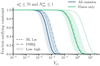 |
Fig. 9. Fraction of simulated surveys satisfying |
| In the text | |
|
Fig. B.1. Per-flavour diffuse neutrino flux used is shown for both the atmospheric and astrophysical components. For the astrophysical case, the two extreme cases also considered bound the shaded region. |
| In the text | |
|
Fig. B.2. Details of the neutrino alert simulations. Left panel: Whole-sky effective area for the HESE and EHE track alerts generated via simulations using the detector mode described in Sect. 3.4. Right panel: Cumulative distribution for the angular resolution of simulated alert events (c.f. Figs. 7 and 9 in Aartsen et al. 2017c). |
| In the text | |
Current usage metrics show cumulative count of Article Views (full-text article views including HTML views, PDF and ePub downloads, according to the available data) and Abstracts Views on Vision4Press platform.
Data correspond to usage on the plateform after 2015. The current usage metrics is available 48-96 hours after online publication and is updated daily on week days.
Initial download of the metrics may take a while.