| Issue |
A&A
Volume 667, November 2022
|
|
|---|---|---|
| Article Number | L2 | |
| Number of page(s) | 10 | |
| Section | Letters to the Editor | |
| DOI | https://doi.org/10.1051/0004-6361/202244169 | |
| Published online | 03 November 2022 | |
Letter to the Editor
Evidence of a signature of planet formation processes from solar neutrino fluxes⋆,⋆⋆
1
Department of Physics, Kurume University, 67 Asahimachi, Kurume, Fukuoka, 830-0011, Japan
e-mail: This email address is being protected from spambots. You need JavaScript enabled to view it.
2
Université Côte d’Azur, Observatoire de la Côte d’Azur, CNRS, Laboratoire Lagrange, Bd de l’Observatoire, CS 34229, 06304 Nice cedex 4, France
3
Département d’Astronomie, Université de Genève, Chemin Pegasi 51, 1290 Versoix, Switzerland
Received:
2
June
2022
Accepted:
7
October
2022
Abstract
Solar evolutionary models are thus far unable to reproduce spectroscopic, helioseismic, and neutrino constraints consistently, resulting in the so-called solar modeling problem. In parallel, planet formation models predict that the evolving composition of the protosolar disk and, thus, of the gas accreted by the proto-Sun must have been variable. We show that solar evolutionary models that include a realistic planet formation scenario lead to an increased core metallicity of up to 5%, implying that accurate neutrino flux measurements are sensitive to the initial stages of the formation of the Solar System. Models with homogeneous accretion match neutrino constraints to no better than 2.7σ. In contrast, accretion with a variable composition due to planet formation processes, leading to metal-poor accretion of the last ∼4% of the young Sun’s total mass, yields solar models within 1.3σ of all neutrino constraints. We thus demonstrate that in addition to increased opacities at the base of the convective envelope, the formation history of the Solar System constitutes a key element in resolving the current crisis of solar models.
Key words: neutrinos / Sun: interior / Sun: evolution / accretion, accretion disks / protoplanetary disks / planets and satellites: formation
Supplemental materials are only available at the CDS via anonymous ftp to cdsarc.cds.unistra.fr (130.79.128.5) or via https://cdsarc.cds.unistra.fr/viz-bin/cat/J/A+A/667/L2 or via https://doi.org/10.5281/zenodo.7156794
Animations associated to Figs. 3 and A.1 are available at https://www.aanda.org
© M. Kunitomo et al. 2022
 Open Access article, published by EDP Sciences, under the terms of the Creative Commons Attribution License (https://creativecommons.org/licenses/by/4.0), which permits unrestricted use, distribution, and reproduction in any medium, provided the original work is properly cited.
This article is published in open access under the Subscribe-to-Open model. This email address is being protected from spambots. You need JavaScript enabled to view it. to support open access publication.
1. Introduction
The Sun is a key piece of the puzzle of the theory of stellar structure and evolution. Due to its proximity, a great wealth of observational data has been acquired (i.e., spectroscopic, helioseismic, and neutrino observations). All these constraints have been extensively used to model our star theoretically using numerical simulations. Good agreement was achieved in the 1990s using so-called standard solar models (solar models constructed with standard input physics; e.g., Christensen-Dalsgaard et al. 1996). In recent years, updates of the solar chemical composition (Asplund et al. 2009, 2021) have significantly worsened the situation. This so-called solar abundance problem has been thoroughly studied in the last two decades, with a clear solution yet to be found (Montalban et al. 2006; Basu & Antia 2008; Buldgen et al. 2019; Orebi Gann et al. 2021; Magg et al. 2022). While the abundance revision triggered the crisis, the issue is actually more of a solar modeling problem, with multiple ingredients called into question.
Apart from abundances, the main suspect has been radiative opacity, which over the course of the history of stellar evolution theory has been known to require significant revisions. A number of studies identified that an increase of ∼10% in the interior opacity would indeed partly alleviate the issue (Bahcall et al. 2005; Ayukov & Baturin 2017; Kunitomo & Guillot 2021). Recently, experimental measurements of iron opacity in almost the same conditions as the solar interior (Bailey et al. 2015) have lent further traction to this hypothesis, even though these results still have to be explained from a theoretical point of view (see, amongst others, Nahar & Pradhan 2016; Iglesias & Hansen 2017).
In addition to microscopic ingredients such as opacity, the recipe of the standard solar model itself is under question. Recently, Eggenberger et al. (2022) showed that including the effects of (magneto)hydrodynamic instabilities in evolutionary computations allows us to simultaneously reproduce the solar internal rotation profile, the surface lithium abundance, and the surface helium abundance, a feat impossible for standard solar models that neglect rotation. This refinement provides only a partial solution to the issue, as it does not improve the agreement of models in terms of sound speed inversions and neutrino fluxes.
The first detection of solar neutrinos was surprising because inferred fluxes were about three times smaller than predicted by standard solar models. This so-called solar neutrino problem was an issue due to a change in the flavor of the neutrinos themselves and is now resolved (e.g., Christensen-Dalsgaard 2021, and references therein). Recent experimental studies have measured neutrinos both from the proton-proton (pp) chain and the carbon-nitrogen-oxygen (CNO) cycle, and the accuracy has been improving (e.g., Agostini et al. 2018; Borexino Collaboration 2020; Orebi Gann et al. 2021). Solar neutrinos are most important because they provide direct access to the solar core: pp, 7Be, and 8B neutrinos provide information on the temperature and temperature gradient in the core, whereas CNO neutrinos provide direct access to the core composition (Haxton & Serenelli 2008; Gough 2019). Although many studies have attempted to account for measured solar neutrino fluxes (e.g., Bahcall et al. 2006), no solar model that uses updated abundances has reproduced both neutrino observations and other constraints simultaneously (e.g., Vinyoles et al. 2017). Matching the observational constraints globally is therefore paramount for progress in our understanding of the composition, evolution, and early history of the Sun.
In this study we combine solar evolutionary models that include the early accretion phase with up-to-date knowledge of planet formation processes to calculate present-day solar models. These models are then compared to all available observational constraints.
2. Calibrating solar models that include disk accretion
We focused on solar models calibrated to match both helioseismic and spectroscopic constraints using an extended procedure (see Appendix A.2 and Table A.1) and examined how they fare against the observed neutrino fluxes (Appendix A.3). We followed the approach of our previous work (Kunitomo & Guillot 2021), where we used solar models computed with the Modules for Experiments in Stellar Astrophysics (MESA) stellar evolution code, taking the progressive accretion of circumstellar disk material onto the proto-Sun into account (Appendix A.1). We adopted the spectroscopic abundances from Asplund et al. (2009, AGSS09 hereafter); this choice did not have an effect on our conclusions. Our extended calibration procedure aims to reproduce six constraints: luminosity, effective temperature, surface helium abundance, the surface abundance ratio of metals to hydrogen, location of the convective-radiative boundary, and relative differences in the sound speed profile. We calibrated three different sets of models, refining the input physics each time. First, standard solar models were considered. Second, we considered nonstandard models, including an opacity increase near the base of the convective envelope, diffusive overshooting, and accretion with a homogeneous composition. Finally, accretion with a variable composition due to planet formation processes was considered.
Several studies (Guzik et al. 2005; Castro et al. 2007; Haxton & Serenelli 2008; Serenelli et al. 2011; Zhang et al. 2019) have indicated that a variation in the accretion metallicity, Zaccretion, would affect the outcome of the calibration. On the basis of models of the evolution of circumstellar disks and of the formation and migration of pebbles, planetesimals, and protoplanets (Garaud 2007), we advocate for the existence of a rapid drift of pebbles (“pebble wave”) followed by a decrease in the metallicity of the accreted gas due to both the early accretion of this dust and the formation of planetesimals and protoplanets (Kunitomo & Guillot 2021). Disk winds, either thermally or magnetically driven, may also selectively remove hydrogen and helium and thus limit the extent and duration of the low-metallicity accretion phase. A comparison of the mass of dust measured in protoplanetary disks and the mass of solids in exoplanets (Manara et al. 2018) suggests that dust growth and the formation of planetesimals must have started early, within a million years of the formation of the central protostars. In our Solar System, isotopic anomalies in meteorites are indicative of the formation of Jupiter’s core ∼1 Myr after the first solids (Kruijer et al. 2020), indicating that an efficient filtering of incoming dust (Guillot et al. 2014) and low-metallicity accretion should have begun at that time. We estimate that 97 to 168 M⊕ of solids should be retained in planets or ejected from the Solar System (Kunitomo et al. 2018). This corresponds to the accretion of ∼2 to 4% of the Sun’s mass in the form of zero-metallicity gas. The presence of a pebble wave leads to an early accretion of solids and thus an increase in this value. Conversely, the selective removal of hydrogen and helium by disk winds lowers this value. Consequently, estimates based on up-to-date simulations of the evolution of disks indicate that between 2 and 5% of the mass last accreted by the Sun should be characterized by a low metallicity (Kunitomo & Guillot 2021). In our best model, the accretion metallicity increases from 0.014 (protosolar mass ≤0.90 M⊙ and time ≤0.7 Myr) to 0.065 (0.96 M⊙ and 2.2 Myr), 0.1 M⊙ metal-free gas is lost by disk winds, and 150 M⊕ of solids are retained in planets, leading to a 0.04 M⊙ metal-free gas in the last phase (see Fig. 3b and Appendix A.4 for a detailed description).
3. Results
In Fig. 1 we compare the neutrino fluxes (Φ(7Be), Φ(8B), Φ(pp), Φ(pep), and Φ(CNO); see Appendix A.3) from observational constraints to those obtained for standard solar models and for models that include an opacity increase. Standard solar models in the literature (Vinyoles et al. 2017; Farag et al. 2020) indicate higher Φ(7Be), Φ(8B), and Φ(CNO) for models with high-metallicity (Z) Grevesse & Sauval (1998, GS98 hereafter) abundances compared to models with low-Z AGSS09 abundances. Our calculations show that this is in fact a calibration issue, linked to the fact that these standard solar models used three constraints as usual in a classical calibration scheme (see Sect. A.2): when using the same approach with the three calibration constraints, we obtain the same results as Farag et al. (2020; see our Fig. 1). Conversely, when including our extended calibration procedure with six constraints (similar to Ayukov & Baturin 2017), the results obtained for GS98 and AGSS09 abundances are found to be close to one another and good matches to the neutrino constraints. However, these models with the AGSS09 composition are poor fits to the spectroscopic and helioseismic constraints (Kunitomo & Guillot 2021), with values of χ2 significantly above unity, illustrating the well-known disagreement between the standard solar models with the AGSS09 abundances and the observations.
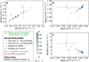 |
Fig. 1. Neutrino fluxes obtained for standard solar models and models with opacity increases. Panels (a)–(c): the neutrino fluxes of Φ(7Be), Φ(8B), Φ(pp), Φ(pep), and Φ(CNO) = Φ(13N) + Φ(15O) + Φ(17F) (see Appendix A.3). The squares and the upward and downward pointing triangles show the standard solar models with three calibration constraints (see Appendix A.2), those from Vinyoles et al. (2017), Farag et al. (2020), and this study, respectively. The open circles show our standard solar models with six constraints. The Φ(pep) and Φ(17F) values are not available in Farag et al. (2020), and thus Φ(CNO) = Φ(13N) + Φ(15O) is used for their models. The blue and red colors indicate the models with low-Z AGSS09 and high-Z GS98 compositions, respectively. The filled circles show our models with opacity increase A2 (=0, 0.04, 0.08, 0.12, 0.15, 0.18, and 0.22), which is shown by the color, with the size χ2, which is ≲0.5 for A2 ∈ [0.12, 0.18]. The green circles with error bars show the observed constraints (Orebi Gann et al. 2021). |
Models that include an opacity increase (parameter A2 corresponds to the relative increase to the standard opacity), shown in Fig. 1, are characterized by lower χ2 values (Bahcall et al. 2005; Ayukov & Baturin 2017; Kunitomo & Guillot 2021), but they depart from the observed neutrino fluxes due to their low central metallicities. Our best models that minimize χ2 (with A2 = 0.12 to 0.18) have a Φ(8B) flux that is 2.7 to 5.1σ lower than the observational constraints, whereas both Φ(pp) and Φ(CNO) are within 1.5 and 1.4σ, respectively. Therefore, although these models match both helioseismic and spectroscopic constraints, they do not account for the observed neutrino fluxes. This is a well-known issue with solar models that led some works to consider low-metallicity accretion to try to recover a “high-Z” radiative interior embedded under a “low-Z” convective envelope (Guzik et al. 2005; Castro et al. 2007).
Thus far, we have only considered solar models that either start with the Sun’s present mass or include the accretion of disk material with a constant metallicity. Figure 2 compares the models with the lowest values of χ2 in Fig. 1 (i.e., those with an opacity increase of A2 ∈ [0.12, 0.18] and homogeneous accretion) with the same models but including accretion with a variable composition. The values of χ2 are almost independent of our choice of the accretion model: the planet formation processes occur while the proto-Sun is still largely convective, implying that most of the solar internal structure is unchanged. However, the values of all neutrino fluxes are affected, indicating that the solar core retains a clear signature of planet formation processes. Values of Φ(8B), Φ(7Be), and Φ(CNO) increase, whereas Φ(pp) and Φ(pep) decrease slightly (Serenelli et al. 2011). This results in models with planet formation processes that fit all the helioseismic, spectroscopic, and neutrino constraints. This is the case for the model with A2 = 0.12, with a worse fit being Φ(pep), which is only 1.3σ lower than the observational constraint.
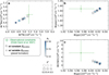 |
Fig. 2. Neutrino fluxes obtained for the models with an opacity increase and planet formation. Shown are the models with an opacity increase (circles; see also Fig. 1) and with both an opacity increase and a variable Zaccretion (i.e., planet formation processes; star symbols). The colors show the opacity increase A2 ∈ [0.12, 0.18]. The opacity increase in this range leads to a better match with spectroscopic and helioseismic observations (χ2 ≲ 0.5 indicated by the size). A higher opacity increase leads to lower Φ(8B), Φ(7Be), and Φ(CNO) values, whereas the planet formation processes lead to higher values. Consequently, our best model with both an opacity increase of A2 = 0.12 and planet formation processes (i.e., star symbol with white color) reproduces not only the observed constraints of neutrino fluxes (green circles with error bars) but also the spectroscopic and helioseismic observations. (See “K2-MZvar-A2-12” and “K2-A2-12” in Table A.1 and the CDS table for more details about the models with A2 = 0.12 and with and without planet formation processes, respectively.) |
The enhancement of the 7Be, 8B, and CNO neutrino fluxes is directly linked to an increased metallicity and temperature of the solar core, which are closely related (see Appendix A.3). As shown in Fig. 3, the pebble wave leads to an initially high metallicity throughout the solar interior (see Figs. 3a and b). The following low-Z accretion phase leads to a decrease in the surface metallicity, which, because of the spectroscopic constraints included in the calibration, becomes indistinguishable from that in the case with homogeneous accretion (Fig. 3c). However, the central region retains memory from the initial high-Z phase because the growth of the central radiative core after 1.7 Myr halts its mixing with the rest of the star (Figs. 3d and e). Between 30 and 100 Myr, an incomplete CNO cycle leads to a transient central convective core (also due to out-of-equilibrium 3He burning) and to a limited increase in the central metallicity. It then progressively increases on timescales of ∼1 Gyr due to gravitational settling. This results in a central metallicity of the present-day Sun that is increased by ≃5% over that of models that do not account for planet formation processes (see Figs. 3f and A.1).
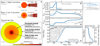 |
Fig. 3. Long-term evolution of models with planet formation processes. Panela: a schematic illustration of the evolution of a model with a variable Zaccretion and an opacity increase of A2 = 0.12. In the early phase, the metallicity of the proto-Sun increases with time due to the high-Z accretion, which results from the dust drift and selective removal of hydrogen and helium by disk winds (see text). Once protoplanets are formed or dust grains in the protosolar disk are exhausted, the disk metallicity decreases, and consequently, the solar surface metallicity, Zsurf, decreases. The signature of this variable Zaccretion remains in the solar core until the solar age. The circles (not to scale) show the solar metallicity profile at times tA = 1.73 Myr, tB = 10 Myr, and t⊙ = 4.567 Gyr. Panelsb–d: the evolution of Zaccretion, Zsurf, and Zcenter of the models with a variable Zaccretion (solid blue lines) and a constant Zaccretion (dotted gray lines), respectively. Panele: the internal structure evolution (the so-called Kippenhahn diagram). The cloudy and white regions show the convective and radiative regions, respectively. The two lines (blue and gray) are almost the same. A radiative core emerges at time tA. The solid black line indicates the stellar mass. Panelf: the metallicity profile of the present-day Sun. Animations that show the metallicity profile in the solar interior of these models are available online and at Zenodo. (See “K2-MZvar-A2-12” and “K2-A2-12” in Table A.1 and the CDS table for more details regarding the models with and without planet formation processes, respectively.) |
We stress that the magnitude of this effect cannot be precisely estimated due to uncertainties in both star and planet formation processes. The duration of the accretion phase may be shorter than assumed here (10 Myr), leading to a smaller increase in the central metallicity (Kunitomo & Guillot 2021). On the other hand, the release of energy by the accretion shock on the proto-Sun could lead to a faster growth of the internal radiative zone after only ∼1 Myr (Kunitomo et al. 2018). Similarly, including mass loss by solar winds leads to a higher mass of the proto-Sun and hence also leads to a faster growth of the radiative zone. Thus, both processes are expected to amplify the change in the central metallicity and neutrino fluxes due to the planet formation processes, regardless of the adopted solar chemical composition.
4. Conclusion
We simulated the evolution of the Sun from the protostellar phase to the present day using all available constraints. Our study demonstrates that planet formation processes have a significant contribution to present-day solar neutrino fluxes. The main conclusions are summarized as follows:
-
The solution depends on the calibration procedure: our models calibrated with six helioseismic and spectroscopic constraints are different from standard solar models calibrated with three constraints.
-
Models that include a localized opacity increase, as indicated by experimental results, match all the helioseismic and spectroscopic constraints. However, due to their low central temperature, they match the neutrino constraints to no better than 2.7σ.
-
The variable composition of accreted gas resulting from planet formation processes induces a higher central metallicity of the present-day Sun by up to 5%, which increases Φ(8B), Φ(7Be), and Φ(CNO) and lowers Φ(pp) and Φ(pep), in agreement with observational requirements. Our best model reproduces all the observed neutrino fluxes within 1.3σ.
In conclusion, despite the uncertainties related to planet formation scenarios, our work shows that neutrino fluxes are intrinsically tied to the evolutionary history of the Sun and that the effects of planet formation should be considered when interpreting these measurements. In our best models, pebble waves and the formation of planets led to a metal-poor accretion of the last 4% of the young Sun’s mass. More accurate neutrino fluxes measurements and constraints on the input physics that affect neutrino fluxes are thus highly desirable.
Movies
Movie 1 associated with Fig. 3 (K2-A2-12) Access Supplementary Material
Movie 2 associated with Fig. 3 (K2-MZvar-A2-12) Access Supplementary Material
Movie 3 associated with Fig. A.1 (K2-A2-12-r-Z) Access Supplementary Material
Movie 4 associated with Fig. A.1 (K2-MZvar-A2-12-r-Z) Access Supplementary Material
Acknowledgments
This work was supported by the JSPS KAKENHI (grant no. 20K14542). Numerical computations were carried out on the PC cluster at the Center for Computational Astrophysics, National Astronomical Observatory of Japan. T.G. acknowledges funding from the Programme National de Planétologie. G.B. acknowledges funding from the SNF AMBIZIONE grant no. 185805 (Seismic inversions and modelling of transport processes in stars). Software: MESA (version 12115; Paxton et al. 2011, 2013, 2015; Paxton et al. 2018, 2019).
References
- Agostini, M., Altenmüller, K., Appel, S., et al. 2018, Nature, 562, 505 [CrossRef] [Google Scholar]
- Aharmim, B., Ahmed, S. N., Anthony, A. E., et al. 2013, Phys. Rev. C, 88, 025501 [NASA ADS] [CrossRef] [Google Scholar]
- Amelin, Y., Krot, A. N., Hutcheon, I. D., & Ulyanov, A. A. 2002, Science, 297, 1678 [NASA ADS] [CrossRef] [Google Scholar]
- Anderson, M., Andringa, S., Asahi, S., et al. 2019, Phys. Rev. D, 99, 012012 [NASA ADS] [CrossRef] [Google Scholar]
- Angulo, C., Arnould, M., Rayet, M., et al. 1999, Nucl. Phys. A, 656, 3 [Google Scholar]
- Appelgren, J., Lambrechts, M., & Johansen, A. 2020, A&A, 638, A156 [NASA ADS] [CrossRef] [EDP Sciences] [Google Scholar]
- Asplund, M., Grevesse, N., Sauval, A. J., & Scott, P. 2009, ARA&A, 47, 481 [NASA ADS] [CrossRef] [Google Scholar]
- Asplund, M., Amarsi, A. M., & Grevesse, N. 2021, A&A, 653, A141 [NASA ADS] [CrossRef] [EDP Sciences] [Google Scholar]
- Ayukov, S. V., & Baturin, V. A. 2017, Astron. Rep., 61, 901 [NASA ADS] [CrossRef] [Google Scholar]
- Bahcall, J. N., & Ulmer, A. 1996, Phys. Rev. D, 53, 4202 [NASA ADS] [CrossRef] [Google Scholar]
- Bahcall, J. N., Basu, S., Pinsonneault, M., & Serenelli, A. M. 2005, ApJ, 618, 1049 [NASA ADS] [CrossRef] [Google Scholar]
- Bahcall, J. N., Serenelli, A. M., & Basu, S. 2006, ApJS, 165, 400 [NASA ADS] [CrossRef] [Google Scholar]
- Bailey, J. E., Nagayama, T., Loisel, G. P., et al. 2015, Nature, 517, 56 [NASA ADS] [CrossRef] [Google Scholar]
- Basu, S., & Antia, H. M. 2004, ApJ, 606, L85 [NASA ADS] [CrossRef] [Google Scholar]
- Basu, S., & Antia, H. M. 2008, Phys. Rep., 457, 217 [Google Scholar]
- Basu, S., Chaplin, W. J., Elsworth, Y., New, R., & Serenelli, A. M. 2009, ApJ, 699, 1403 [NASA ADS] [CrossRef] [Google Scholar]
- Bergström, J., Gonzalez-Garcia, M. C., Maltoni, M., et al. 2016, J. High Energy Phys., 2016, 132 [CrossRef] [Google Scholar]
- Boothroyd, A. I., & Sackmann, I. J. 2003, ApJ, 583, 1004 [NASA ADS] [CrossRef] [Google Scholar]
- Borexino Collaboration (Agostini, M., et al.) 2020, Nature, 587, 577 [NASA ADS] [CrossRef] [Google Scholar]
- Buldgen, G., Salmon, S., & Noels, A. 2019, Front. Astron. Space Sci., 6, 42 [NASA ADS] [CrossRef] [Google Scholar]
- Castro, M., Vauclair, S., & Richard, O. 2007, A&A, 463, 755 [NASA ADS] [CrossRef] [EDP Sciences] [Google Scholar]
- Christensen-Dalsgaard, J. 2021, Liv. Rev. Sol. Phys., 18, 2 [NASA ADS] [CrossRef] [Google Scholar]
- Christensen-Dalsgaard, J., Dappen, W., Ajukov, S. V., et al. 1996, Science, 272, 1286 [Google Scholar]
- Chugunov, A. I., Dewitt, H. E., & Yakovlev, D. G. 2007, Phys. Rev. D, 76, 025028 [NASA ADS] [CrossRef] [Google Scholar]
- Cox, J., & Giuli, R. 1968, Principles of Stellar Structure (New York: Gordon and Breach), 401 [Google Scholar]
- Eggenberger, P., Buldgen, G., Salmon, S. J. A. J., et al. 2022, Nat. Astron., 6, 788 [NASA ADS] [CrossRef] [Google Scholar]
- Elbakyan, V. G., Johansen, A., Lambrechts, M., Akimkin, V., & Vorobyov, E. I. 2020, A&A, 637, A5 [NASA ADS] [CrossRef] [EDP Sciences] [Google Scholar]
- Farag, E., Timmes, F. X., Taylor, M., Patton, K. M., & Farmer, R. 2020, ApJ, 893, 133 [CrossRef] [Google Scholar]
- Gando, A., Gando, Y., Hanakago, H., et al. 2015, Phys. Rev. C, 92, 055808 [NASA ADS] [CrossRef] [Google Scholar]
- Garaud, P. 2007, ApJ, 671, 2091 [NASA ADS] [CrossRef] [Google Scholar]
- Gough, D. O. 2019, MNRAS, 485, L114 [NASA ADS] [CrossRef] [Google Scholar]
- Grevesse, N., & Sauval, A. J. 1998, Space Sci. Rev., 85, 161 [Google Scholar]
- Guillot, T., & Hueso, R. 2006, MNRAS, 367, L47 [CrossRef] [Google Scholar]
- Guillot, T., Ida, S., & Ormel, C. W. 2014, A&A, 572, A72 [NASA ADS] [CrossRef] [EDP Sciences] [Google Scholar]
- Guzik, J. A., Willson, L. A., & Brunish, W. M. 1987, ApJ, 319, 957 [NASA ADS] [CrossRef] [Google Scholar]
- Guzik, J. A., Watson, L. S., & Cox, A. N. 2005, ApJ, 627, 1049 [NASA ADS] [CrossRef] [Google Scholar]
- Hartmann, L., Calvet, N., Gullbring, E., & D’Alessio, P. 1998, ApJ, 495, 385 [Google Scholar]
- Haxton, W. C., & Serenelli, A. M. 2008, ApJ, 687, 678 [NASA ADS] [CrossRef] [Google Scholar]
- Herwig, F. 2000, A&A, 360, 952 [NASA ADS] [Google Scholar]
- Iben, I., Jr 1965, ApJ, 141, 993 [NASA ADS] [CrossRef] [Google Scholar]
- Iglesias, C. A., & Hansen, S. B. 2017, ApJ, 835, 284 [NASA ADS] [CrossRef] [Google Scholar]
- Imbriani, G., Costantini, H., Formicola, A., et al. 2005, Eur. Phys. J. A, 25, 455 [Google Scholar]
- Kippenhahn, R., & Weigert, A. 1990, Stellar Structure and Evolution (Springer-Verlag) [Google Scholar]
- Kruijer, T. S., Kleine, T., & Borg, L. E. 2020, Nat. Astron., 4, 32 [Google Scholar]
- Kunitomo, M., & Guillot, T. 2021, A&A, 655, A51 [NASA ADS] [CrossRef] [EDP Sciences] [Google Scholar]
- Kunitomo, M., Guillot, T., Takeuchi, T., & Ida, S. 2017, A&A, 599, A49 [NASA ADS] [CrossRef] [EDP Sciences] [Google Scholar]
- Kunitomo, M., Guillot, T., Ida, S., & Takeuchi, T. 2018, A&A, 618, A132 [NASA ADS] [CrossRef] [EDP Sciences] [Google Scholar]
- Kunitomo, M., Suzuki, T. K., & Inutsuka, S.-I. 2020, MNRAS, 492, 3849 [CrossRef] [Google Scholar]
- Le Pennec, M., Turck-Chièze, S., Salmon, S., et al. 2015, ApJ, 813, L42 [Google Scholar]
- Magg, E., Bergemann, M., Serenelli, A., et al. 2022, A&A, 661, A140 [NASA ADS] [CrossRef] [EDP Sciences] [Google Scholar]
- Manara, C. F., Morbidelli, A., & Guillot, T. 2018, A&A, 618, L3 [NASA ADS] [CrossRef] [EDP Sciences] [Google Scholar]
- Montalban, J., Miglio, A., Theado, S., Noels, A., & Grevesse, N. 2006, Commun. Asteroseismol., 147, 80 [Google Scholar]
- Nahar, S. N., & Pradhan, A. K. 2016, Phys. Rev. Lett., 116, 235003 [Google Scholar]
- Nelder, J. A., & Mead, R. 1965, Comput. J., 7, 308 [Google Scholar]
- Orebi Gann, G. D., Zuber, K., Bemmerer, D., & Serenelli, A. 2021, Ann. Rev. Nucl. Part. Sci., 71, 491 [NASA ADS] [CrossRef] [Google Scholar]
- Particle Data Group (Zyla, P. A., et al.) 2020, Prog. Theor. Exp. Phys., 2020, 083C01 [CrossRef] [Google Scholar]
- Paxton, B., Bildsten, L., Dotter, A., et al. 2011, ApJS, 192, 3 [Google Scholar]
- Paxton, B., Cantiello, M., Arras, P., et al. 2013, ApJS, 208, 4 [Google Scholar]
- Paxton, B., Marchant, P., Schwab, J., et al. 2015, ApJS, 220, 15 [Google Scholar]
- Paxton, B., Schwab, J., Bauer, E. B., et al. 2018, ApJS, 234, 34 [NASA ADS] [CrossRef] [Google Scholar]
- Paxton, B., Smolec, R., Schwab, J., et al. 2019, ApJS, 243, 10 [Google Scholar]
- Sackmann, I. J., & Boothroyd, A. I. 2003, ApJ, 583, 1024 [NASA ADS] [CrossRef] [Google Scholar]
- Salmon, S. J. A. J., Buldgen, G., Noels, A., et al. 2021, A&A, 651, A106 [NASA ADS] [CrossRef] [EDP Sciences] [Google Scholar]
- Sato, T., Okuzumi, S., & Ida, S. 2016, A&A, 589, A15 [NASA ADS] [CrossRef] [EDP Sciences] [Google Scholar]
- Serenelli, A. M., Haxton, W. C., & Peña-Garay, C. 2011, ApJ, 743, 24 [NASA ADS] [CrossRef] [Google Scholar]
- Thoul, A. A., Bahcall, J. N., & Loeb, A. 1994, ApJ, 421, 828 [Google Scholar]
- Tsukamoto, Y., Okuzumi, S., & Kataoka, A. 2017, ApJ, 838, 151 [NASA ADS] [CrossRef] [Google Scholar]
- Vescovi, D., Piersanti, L., Cristallo, S., et al. 2019, A&A, 623, A126 [NASA ADS] [CrossRef] [EDP Sciences] [Google Scholar]
- Villante, F. L., & Serenelli, A. 2021, Front. Astron. Space Sci., 7, 112 [Google Scholar]
- Vinyoles, N., Serenelli, A. M., Villante, F. L., et al. 2017, ApJ, 835, 202 [NASA ADS] [CrossRef] [Google Scholar]
- Wood, B. E., Müller, H.-R., Zank, G. P., Linsky, J. L., & Redfield, S. 2005, ApJ, 628, L143 [NASA ADS] [CrossRef] [Google Scholar]
- Zhang, Q.-S., Li, Y., & Christensen-Dalsgaard, J. 2019, ApJ, 881, 103 [Google Scholar]
Appendix A: Methods
A.1. Calculation of solar structure and evolution models
This section describes how we simulated the formation and evolution of the Sun. We followed Sect. 3 of Kunitomo & Guillot (2021) for the modeling unless otherwise noted. For more details, we refer readers to Kunitomo et al. (2017), Kunitomo et al. (2018), and Paxton et al. (2011, 2013, 2015, 2018, 2019). Our models were calculated using the MESA stellar evolution code (Paxton et al. 2011, 2013, 2015; Paxton et al. 2018, 2019). The models of nuclear reactions and accretion are discussed below. We modeled the opacity increase as a function of temperature. Since the contribution of iron to the Rosseland-mean opacity has a Gaussian form with temperature (Le Pennec et al. 2015), we adopted the Gaussian function centered at T = 106.45 K with varying amplitude, A2 (see Eq. 5 of Kunitomo & Guillot 2021). Convection is modeled with the mixing-length theory from Cox & Giuli (1968). Diffusive convective overshooting is also considered with the model in Herwig (2000) both below a convective envelope and above a convective core. Element diffusion is calculated with the formalism in Thoul et al. (1994).
There are four differences from standard solar models (e.g., Vinyoles et al. 2017; Farag et al. 2020): namely, the calibration procedure, diffusive overshooting, opacity increase, and accretion that has a variable composition. We included planet formation processes based on recent progress, which differs from previous studies, including low-metallicity accretion (see below). We note that although Eggenberger et al. (2022) recently showed the impact of (magneto)hydrodynamic instabilities driven by rotation on the internal rotation and lithium abundance, they do not improve sound speed inversions and neutrino fluxes, and thus, we do not account for these instabilities.
A.2. Calibration procedure
In each model, input parameters are calibrated to minimize the reduced χ2 value defined as ![Mathematical equation: $ \chi^2 = {\sum_{i=1}^N \left[ (q_i-q_{i,\rm target})/\sigma(q_i)\right]^2}/{N} $](/articles/aa/full_html/2022/11/aa44169-22/aa44169-22-eq1.gif) , where N is the number of constraints, qi is the simulation result, and qi,target and σ are the observational constraint and its uncertainty, respectively. We adopted N = 6 for the models with an “extended” calibration procedure (similar to Ayukov & Baturin 2017) and N = 3 (i.e., (Z/X)surf, L⋆, Teff; see below) for the standard solar models. Using the downhill simplex method (Nelder & Mead 1965), we searched for a set of input parameters that minimizes χ2. We assumed that the solar age is 4.567 Gyr (Amelin et al. 2002). The input parameters include two parameters for convection (mixing length and overshooting) and parameters for the initial composition, opacity increase, and accretion, which vary from model to model.
, where N is the number of constraints, qi is the simulation result, and qi,target and σ are the observational constraint and its uncertainty, respectively. We adopted N = 6 for the models with an “extended” calibration procedure (similar to Ayukov & Baturin 2017) and N = 3 (i.e., (Z/X)surf, L⋆, Teff; see below) for the standard solar models. Using the downhill simplex method (Nelder & Mead 1965), we searched for a set of input parameters that minimizes χ2. We assumed that the solar age is 4.567 Gyr (Amelin et al. 2002). The input parameters include two parameters for convection (mixing length and overshooting) and parameters for the initial composition, opacity increase, and accretion, which vary from model to model.
In the calibration procedure, simulation results were compared with the six constraints from spectroscopic and helioseismic observations summarized in Table A.1 (see also Table 3 of Kunitomo & Guillot 2021): surface abundance ratio of metals to hydrogen (Z/X)surf, surface helium abundance Ysurf, location of the convective-radiative boundary RCZ, root-mean-square sound speed rms(δcs), luminosity L⋆ (=L⊙ ± 0.01 dex), and effective temperature Teff (=5777 ± 10 K). We note that the current uncertainty in the surface metallicity of the Sun (Asplund et al. 2021; Magg et al. 2022) does not affect the conclusions of our study; a thorough discussion is beyond the scope of this work, which instead focuses on the effect of planet formation processes.
Results minimized by the chi-squared simulations and observational constraints.
Table A.1 also summarizes the results of our models and previous studies. The SSM-AGSS09 and SSM-GS98 models are our standard solar models following Farag et al. (2020) (i.e., N = 3) with the AGSS09 and GS98 abundances, respectively. The noacc-noov and noacc-GS98-noov models (open circles in Figs. 1 and A.4e) are the models with the extended calibration (N = 6) without overshooting. The model with opacity increase (A2 = 0.12) and overshooting is denoted K2-A2-12 (filled circles in Figs. 1 and 2), whereas the same model but with planet formation processes is denoted K2-MZvar-A2-12 (star symbols in Fig. 2). Additional supplemental materials showing the details of the results of the optimized models are available at the CDS and Zenodo (see the links provided in the footnote on the first page).
We note that Haxton & Serenelli (2008) investigated the dependence of neutrino fluxes on parameters by using the results of standard solar models and derived their relations assuming the linearity of the dependence. In contrast, we performed evolutionary simulations with the iterative calibration procedure in order to self-consistently track the evolution history, including the effects of planet formation processes in the early phase, and to obtain a global structure of the present-day solar interior model that matches all the spectroscopic, helioseismic, and neutrino constraints.
A.3. Nuclear reactions and neutrinos
Solar neutrinos are emitted by two types of thermonuclear reactions, namely the pp chain and the CNO cycle. The pp chain is
 (A.1)
(A.1)
where p is a proton and d is a deuterium atom. Another known neutrino-emitting reaction is 3He(p, e+ν)4He, but it is extremely rare in the current Sun (Vinyoles et al. 2017; Agostini et al. 2018). The fluxes of neutrinos ν1, ν2, ν3, and ν4 observed on Earth are denoted by Φ(pp), Φ(pep), Φ(7Be), and Φ(8B), respectively. The two branches of the CNO cycle are
 (A.2)
(A.2)
 (A.3)
(A.3)
The fluxes of ν5, ν6, and ν7 are Φ(13N), Φ(15O), and Φ(17F), respectively. We define Φ(CNO) as Φ(13N) + Φ(15O)+Φ(17F) unless otherwise noted.
Neutrino fluxes depend on abundances and temperature. The following fluxes are in particular strongly sensitive to temperature as Φ(7Be) ∝ XcenterZcenterTcenter11, Φ(8B) ∝ XcenterZcenterTcenter25, and Φ(13N),Φ(15O) ∝ XcenterZcenterTcenter20 (Bahcall & Ulmer 1996). In contrast, Φ(pp) is more sensitive to the hydrogen abundance and less sensitive to temperature as ∝ Xcenter2Tcenter4 (Kippenhahn & Weigert 1990). Therefore, in the models with a higher Zcenter and Tcenter, Φ(7Be), Φ(8B), and Φ(CNO) are higher, whereas such models have a lower hydrogen abundance Xcenter and thus a lower Φ(pp) to satisfy the constraint L⋆ = L⊙ at the solar age (see Figs. 1 and 2).
We note that Zcenter and Tcenter are closely related, as follows. A higher Zcenter leads to a higher central opacity, κcenter, because metals dominantly contribute to the opacity. With a higher κcenter, the temperature gradient needs to be higher to flow out the luminosity in the radiative core (Kippenhahn & Weigert 1990), and thus Tcenter is higher.
In the main branch of the CNO cycle (Eq. A.2), the bottleneck reaction is 14N(p, γ)15O. Although the CNO cycle produces only a small fraction (≈1%) of energy in 1 M⊙ stars because of a slightly low Tcenter, a tentative “incomplete CNO cycle” occurs from 30 to 100 Myr. This leads to the conversion of preexisting 12C and 2p into 14N, and thus, the central metallicity, Zcenter, is increased (see Eq. A.2 and Fig. 3d). The CNO cycle has another important implication: it leads to a sharp temperature gradient in the core and thus results in the presence of a convective core (Iben 1965). In our best model, the central region has a composition gradient in the pre-main-sequence phase, and thus, mixing in the core leads to an increase in metallicity at 30 Myr (see Figs. 3d and A.1), whereas this Zcenter modification at 30 Myr does not appear in our model with a homogeneous Zaccretion.
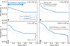 |
Fig. A.1. Evolution of the metallicity profile with mass coordinate. The solid blue and dashed gray lines show the K2-MZvar-A2-12 and K2-A2-12 models, respectively, at 10 Myr (end of the accretion phase; panel a), 100 Myr (b), 1 Gyr (c), and 4.567 Gyr (solar age; d). Animations showing the metallicity profile in the solar interior of these models are available online and at Zenodo. |
We adopted the nuclear reaction rates from NACRE (Angulo et al. 1999) and Imbriani et al. (2005) for the reaction rate of 14N(p, γ)15O. To output neutrino fluxes, we used the subroutine provided in Farag et al. (2020) with a minor update to output Φ(17F). The electron screening formalism of Chugunov et al. (2007) was used. We also mention that the neutrino fluxes are sensitive to the uncertainties in the nuclear reaction rates, as well as electron screening, opacity tables, and the transport of chemical elements over the course of solar evolution (Boothroyd & Sackmann 2003; Salmon et al. 2021; Vescovi et al. 2019; Villante & Serenelli 2021; Eggenberger et al. 2022), and thus could be affected by potential future revisions of these ingredients.
The calibrated models are compared with observed neutrino fluxes in Figs. 1 and 2. Much effort has been made in experiments around the world to constrain the solar neutrino fluxes. We adopted the Φ(pp), Φ(pep), Φ(8B), and Φ(7Be) values from Bergström et al. (2016) and Orebi Gann et al. (2021), which were derived using all the data available up to 2016, whereas we adopted the recent constraint in Borexino Collaboration (2020) for Φ(CNO). We note that there remain relatively large uncertainties in the observed fluxes (partially originated from the uncertainties in the neutrino oscillation model) and that a disagreement between various works is still being debated (Particle Data Group et al. 2020; Orebi Gann et al. 2021, see Fig. A.2). However, discussing these uncertainties is beyond the scope of our work. Nevertheless, future experiments to constrain the fluxes more precisely are thus highly encouraged.
A.4. Planet formation processes
We followed Kunitomo & Guillot (2021) for accretion processes onto the proto-Sun: we started with calculations from a protostellar phase with a seed of mass Mseed = 0.1 M⊙ and metallicity Zseed = 0.02. We adopted the accretion rate, Ṁacc, based on observations (Hartmann et al. 1998): it decreases with time and stops at 10 Myr. We considered heat injection by accreted materials (Kunitomo et al. 2017; Kunitomo & Guillot 2021). We did not consider mass loss by solar winds in the main-sequence phase (Guzik et al. 1987; Sackmann & Boothroyd 2003; Wood et al. 2005; Zhang et al. 2019).
In the models with planet formation processes, the composition of the accreted materials (Xaccretion, Yaccretion, and Zaccretion for the mass fractions of hydrogen, helium, and metals, respectively) vary with time. In the models without them, we adopted a constant composition with time as Xaccretion = Xproto, Yaccretion = Yproto, and Zaccretion = Zproto.
We modeled planet formation processes as a time-dependent Zaccretion based on recent planet formation theory following Kunitomo & Guillot (2021) (see also Fig. 3b). In the earliest phase, the disk gas has a primordial composition (i.e., Xproto, Yproto, and Zproto). Then, we considered a high Zaccretion value due to dust drift (Appelgren et al. 2020; Elbakyan et al. 2020) and/or disk winds (Guillot & Hueso 2006; Kunitomo et al. 2020). In the last phase, Zaccretion = 0 due to the depletion or filtration of pebbles by a planetary gap (Guillot et al. 2014; Sato et al. 2016). In the models with planet formation, three input parameters are calibrated in addition to those for the primordial composition and convection: namely, the stellar masses when Zaccretion increases and decreases (M1 and M2, respectively) and the maximum value of Zaccretion, Zacc, max.
We note that Zaccretion must be consistent with the observations of the Solar System planets and planet formation theory. The total mass of metals in the Solar System planets, MZ, planet, is estimated to be between 97 and 168 M⊕ (Kunitomo et al. 2018). Recent studies have suggested that dust grains grow in the protostellar phase (Manara et al. 2018; Tsukamoto et al. 2017) and a proto-Jupiter was formed early, ∼1 Myr after the Ca-Al-rich inclusions (CAIs) condensed (Kruijer et al. 2020), implying low M1 and M2 values. The total mass lost by disk winds, MXY, lost, is still uncertain, but a recent study (Kunitomo et al. 2020) suggested that it can be ∼0.1 M⊙ around a 1 M⊙ star. If we neglect the early high-Z accretion phase (pebble wave) and assume Zproto ≈ 0.015, this leads to a ≈0.03 M⊙ low-Z accretion in the late phase (i.e., M2 ≈ 0.97 M⊙). Under the fixed value of Zproto, the pebble wave leads to a lower M2, whereas metal-poor disk winds lead to a higher M2. In our best model (see “K2-MZvar-A2-12” in Table A.1 and the CDS table), Zproto = 0.014, Zacc, max = 0.065, M1 = 0.90 M⊙, M2 = 0.96 M⊙, MXY, lost = 0.10 M⊙, and MZ, planet = 150 M⊕.
Figure A.1 shows how the signature of planet formation processes remains in the metallicity profile of the present-day Sun (especially ≲0.2 M⊙). At the end of the accretion phase (=10 Myr), a nonhomogeneous metallicity profile due to the time-dependent Zaccretion exists in the radiative core (≲0.5 M⊙). In particular, high-Z accretion is imprinted below 0.05 M⊙. The central region (≲0.1 M⊙) is subject to an incomplete CNO cycle between 30 and 100 Myr that leads to the convective mixing and a metallicity increase of ∼5 × 10⁻⁴. Gravitational settling takes effect on a timescale of ∼1 Gyr leading to an increase in the central metallicity of ∼5 × 10⁻⁴. Therefore, the central composition of the present-day Sun is determined by accretion, convective mixing, nuclear reactions, and element diffusion.
We note that MXY, lost, MZ, planet, Zproto, and Zacc, max are linked by mass conservation (Kunitomo & Guillot 2021):
 (A.4)
(A.4)
In the early phase in which the proto-Sun is fully convective (i.e., when the protosolar mass M⋆ < 0.95 M⊙), the accretion history is lost. This implies that solutions are highly degenerate: an increase in the metallicity due to a pebble wave that occurs during that phase is indistinguishable from the accretion of gas with a constant metallicity, as long as the total amount of heavy elements accreted over the period is identical (see Fig. A.3). For example, our best model (MXY, lost = 0.1 M⊙, Zacc, max = 0.065, Zproto = 0.014) is approximately equivalent to a simplified model with M1 = M2 = 0.96 M⊙, Zproto = 0.016, and MXY, lost ≃ 0. Therefore, a large variety of solutions that lead to an increased central metallicity and neutrino fluxes agreeing with observations are possible.
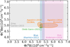 |
Fig. A.2. Observational constraints on the Φ(8B) and Φ(7Be) values. The green open circle with error bars shows the constraints derived using all experimental neutrino data available up to 2016 (Bergström et al. 2016; Orebi Gann et al. 2021), which is used in this study. The orange ellipses show the constraints in Agostini et al. (2018) from the Borexino experiments only (right) and from using available experimental data (left). The gray, blue, and pink shaded regions indicate the constraints from the KamLAND experiments (Gando et al. 2015), from Aharmim et al. (2013) with the Sudbury Neutrino Observatory (SNO), and from Anderson et al. (2019) with the SNO+, respectively. |
To quantify the magnitude of the increased Zcenter by planet formation processes, we performed additional simulations (model “M2var”) for various M2 values. For simplicity, we neglected the high-Z accretion phase (i.e., Zaccretion = Zproto for M⋆ < M2 and Zaccretion = 0 for M⋆ > M2) and investigated the dependence of Zcenter on M2 ∈ [0.92 M⊙, 1 M⊙]. In addition, we neglected overshooting and fixed A2 = 0.12. Figure A.4 shows that a lower M2, which corresponds to a higher mass retained in planets, leads to a higher Zcenter and higher fluxes of Φ(8B), Φ(7Be), and Φ(CNO). However, this effect saturates at M2 = 0.96 M⊙. This mass approximately corresponds to the timing when a radiative core develops (1.7 Myr). In the models with a lower M2 < 0.96 M⊙, a higher Zproto value is needed to reproduce the (Z/X)surf constraint, and thus, the total metal mass in the proto-Sun at 1.7 Myr does not depend on M2. Therefore, the formation of giant planets in the early phase (≲2 Myr), suggested by recent studies, is preferable to induce a high Zcenter value and explain the observed neutrino fluxes. From a linear regression analysis, we obtain the empirical relation
![Mathematical equation: $$ \begin{aligned} {Z_{\rm center}} = \min \left[0.01727,\ 0.01727- 0.0212 \left( M_2/{M_{\odot }} - 0.960 \right) \right]\,. \end{aligned} $$](/articles/aa/full_html/2022/11/aa44169-22/aa44169-22-eq10.gif) (A.5)
(A.5)
In our M2var model, Φ(CNO) has a positive correlation with Zcenter. Recently, Gough (2019) suggested a relation Φ(CNO)/(108 cm−2 s−1) = 250 Zcenter based on standard solar models (Vinyoles et al. 2017). Our models follow a different relation (Φ(CNO)/(108 cm−2 s−1) = 463 Zcenter − 2.88; see Fig. A.4e) due to the different calibration procedures and the accretion history, which are not taken into account in the evolution of standard solar models.
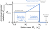 |
Fig. A.3. Time evolution of the metallicity of accreted gas. The blue line indicates our fiducial Zaccretion model, where it increases from Zproto at M⋆ = M1 to Zacc, max at M2 followed by a metal-poor accretion phase. The black line indicates the simplified model (model M2var; see Fig. A.4), which has the same M2 and the total amount of accreted metals as the blue line. If this M2 value is lower than 0.96 M⊙ (which approximately corresponds to when the radiative core develops), then these two models lead to the same Zcenter. |
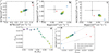 |
Fig. A.4. Neutrino fluxes and central metallicity of the models with different planet formation scenarios. The color of the filled circles (model M2var) corresponds to the M2 value (see panel (d)), which is the protosolar mass when the accretion metallicity decreases. The dotted line in panel (e) shows the relation in Gough (2019), and the dashed lines in panels (d) and (e) show the fits of our M2var models. The black circles with error bars show the observed constraints. The red and blue points indicate the models with the old high-Z GS98 composition and the low-Z AGSS09 composition, respectively. |
All Tables
Results minimized by the chi-squared simulations and observational constraints.
All Figures
|
Fig. 1. Neutrino fluxes obtained for standard solar models and models with opacity increases. Panels (a)–(c): the neutrino fluxes of Φ(7Be), Φ(8B), Φ(pp), Φ(pep), and Φ(CNO) = Φ(13N) + Φ(15O) + Φ(17F) (see Appendix A.3). The squares and the upward and downward pointing triangles show the standard solar models with three calibration constraints (see Appendix A.2), those from Vinyoles et al. (2017), Farag et al. (2020), and this study, respectively. The open circles show our standard solar models with six constraints. The Φ(pep) and Φ(17F) values are not available in Farag et al. (2020), and thus Φ(CNO) = Φ(13N) + Φ(15O) is used for their models. The blue and red colors indicate the models with low-Z AGSS09 and high-Z GS98 compositions, respectively. The filled circles show our models with opacity increase A2 (=0, 0.04, 0.08, 0.12, 0.15, 0.18, and 0.22), which is shown by the color, with the size χ2, which is ≲0.5 for A2 ∈ [0.12, 0.18]. The green circles with error bars show the observed constraints (Orebi Gann et al. 2021). |
| In the text | |
|
Fig. 2. Neutrino fluxes obtained for the models with an opacity increase and planet formation. Shown are the models with an opacity increase (circles; see also Fig. 1) and with both an opacity increase and a variable Zaccretion (i.e., planet formation processes; star symbols). The colors show the opacity increase A2 ∈ [0.12, 0.18]. The opacity increase in this range leads to a better match with spectroscopic and helioseismic observations (χ2 ≲ 0.5 indicated by the size). A higher opacity increase leads to lower Φ(8B), Φ(7Be), and Φ(CNO) values, whereas the planet formation processes lead to higher values. Consequently, our best model with both an opacity increase of A2 = 0.12 and planet formation processes (i.e., star symbol with white color) reproduces not only the observed constraints of neutrino fluxes (green circles with error bars) but also the spectroscopic and helioseismic observations. (See “K2-MZvar-A2-12” and “K2-A2-12” in Table A.1 and the CDS table for more details about the models with A2 = 0.12 and with and without planet formation processes, respectively.) |
| In the text | |
|
Fig. 3. Long-term evolution of models with planet formation processes. Panela: a schematic illustration of the evolution of a model with a variable Zaccretion and an opacity increase of A2 = 0.12. In the early phase, the metallicity of the proto-Sun increases with time due to the high-Z accretion, which results from the dust drift and selective removal of hydrogen and helium by disk winds (see text). Once protoplanets are formed or dust grains in the protosolar disk are exhausted, the disk metallicity decreases, and consequently, the solar surface metallicity, Zsurf, decreases. The signature of this variable Zaccretion remains in the solar core until the solar age. The circles (not to scale) show the solar metallicity profile at times tA = 1.73 Myr, tB = 10 Myr, and t⊙ = 4.567 Gyr. Panelsb–d: the evolution of Zaccretion, Zsurf, and Zcenter of the models with a variable Zaccretion (solid blue lines) and a constant Zaccretion (dotted gray lines), respectively. Panele: the internal structure evolution (the so-called Kippenhahn diagram). The cloudy and white regions show the convective and radiative regions, respectively. The two lines (blue and gray) are almost the same. A radiative core emerges at time tA. The solid black line indicates the stellar mass. Panelf: the metallicity profile of the present-day Sun. Animations that show the metallicity profile in the solar interior of these models are available online and at Zenodo. (See “K2-MZvar-A2-12” and “K2-A2-12” in Table A.1 and the CDS table for more details regarding the models with and without planet formation processes, respectively.) |
| In the text | |
|
Fig. A.1. Evolution of the metallicity profile with mass coordinate. The solid blue and dashed gray lines show the K2-MZvar-A2-12 and K2-A2-12 models, respectively, at 10 Myr (end of the accretion phase; panel a), 100 Myr (b), 1 Gyr (c), and 4.567 Gyr (solar age; d). Animations showing the metallicity profile in the solar interior of these models are available online and at Zenodo. |
| In the text | |
|
Fig. A.2. Observational constraints on the Φ(8B) and Φ(7Be) values. The green open circle with error bars shows the constraints derived using all experimental neutrino data available up to 2016 (Bergström et al. 2016; Orebi Gann et al. 2021), which is used in this study. The orange ellipses show the constraints in Agostini et al. (2018) from the Borexino experiments only (right) and from using available experimental data (left). The gray, blue, and pink shaded regions indicate the constraints from the KamLAND experiments (Gando et al. 2015), from Aharmim et al. (2013) with the Sudbury Neutrino Observatory (SNO), and from Anderson et al. (2019) with the SNO+, respectively. |
| In the text | |
|
Fig. A.3. Time evolution of the metallicity of accreted gas. The blue line indicates our fiducial Zaccretion model, where it increases from Zproto at M⋆ = M1 to Zacc, max at M2 followed by a metal-poor accretion phase. The black line indicates the simplified model (model M2var; see Fig. A.4), which has the same M2 and the total amount of accreted metals as the blue line. If this M2 value is lower than 0.96 M⊙ (which approximately corresponds to when the radiative core develops), then these two models lead to the same Zcenter. |
| In the text | |
|
Fig. A.4. Neutrino fluxes and central metallicity of the models with different planet formation scenarios. The color of the filled circles (model M2var) corresponds to the M2 value (see panel (d)), which is the protosolar mass when the accretion metallicity decreases. The dotted line in panel (e) shows the relation in Gough (2019), and the dashed lines in panels (d) and (e) show the fits of our M2var models. The black circles with error bars show the observed constraints. The red and blue points indicate the models with the old high-Z GS98 composition and the low-Z AGSS09 composition, respectively. |
| In the text | |
Current usage metrics show cumulative count of Article Views (full-text article views including HTML views, PDF and ePub downloads, according to the available data) and Abstracts Views on Vision4Press platform.
Data correspond to usage on the plateform after 2015. The current usage metrics is available 48-96 hours after online publication and is updated daily on week days.
Initial download of the metrics may take a while.