| Issue |
A&A
Volume 667, November 2022
|
|
|---|---|---|
| Article Number | A119 | |
| Number of page(s) | 32 | |
| Section | Interstellar and circumstellar matter | |
| DOI | https://doi.org/10.1051/0004-6361/202243927 | |
| Published online | 17 November 2022 | |
Tracing the contraction of the pre-stellar core L1544 with HC17O+ J = 1–0 emission★
1
Centre for Astrochemical Studies, Max-Planck-Instiut für extraterrestrische Physik,
Giessenbachstr. 1,
85748
Garching, Germany
e-mail: This email address is being protected from spambots. You need JavaScript enabled to view it.
2
Scuola Normale Superiore,
Piazza dei Cavalieri 7,
56126
Pisa, Italy
3
Dipartimento di Chimica “G. Ciamician”,
via F. Selmi 2,
40126
Bologna, Italy
4
IPR, Université de Rennes,
Bât. 11b, Campus de Beaulieu, 263 avenue du Général Leclerc,
35042
Rennes Cedex, France
Received:
2
May
2022
Accepted:
6
September
2022
Abstract
Context. Spectral line profiles of several molecules observed towards the pre-stellar core L1544 appear double-peaked. For abundant molecular species this line morphology has been linked to self-absorption. However, the physical process behind the double-peaked morphology for less abundant species is still under debate.
Aims. In order to understand the cause behind the double-peaked spectra of optically thin transitions and their link to the physical structure of pre-stellar cores, we present high-sensitivity and high spectral resolution HC17O+ J =1−0 observations towards the dust peak in L1544.
Methods. We observed the HC17O+(1−0) spectrum with the Institut de Radioastronomie Millimétrique (IRAM) 30 m telescope. By using state-of-the-art collisional rate coefficients, a physical model for the core and the fractional abundance profile of HC17O+, the hyperfine structure of this molecular ion is modelled for the first time with the radiative transfer code loc applied to the predicted chemical structure of a contracting pre-stellar core. We applied the same analysis to the chemically related C17O molecule.
Results. The observed HC17O+(1−0) and C17O(1−0) lines were successfully reproduced with a non-local thermal equilibrium (LTE) radiative transfer model applied to chemical model predictions for a contracting pre-stellar core. An upscaled velocity profile (by 30%) is needed to reproduce the HC17O+(1−0) observations.
Conclusions. The double peaks observed in the HC17O+(1−0) hyperfine components are due to the contraction motions at densities close to the critical density of the transition (~105 cm−3) and to the decreasing HCO+ fractional abundance towards the centre.
Key words: ISM: molecules / ISM: clouds / radio lines: ISM / stars: formation / radiative transfer
Based on observations carried out with the IRAM 30 m Telescope. IRAM is supported by INSU/CNRS (France), MPG (Germany) and IGN (Spain).
© J. Ferrer Asensio et al. 2022
 Open Access article, published by EDP Sciences, under the terms of the Creative Commons Attribution License (https://creativecommons.org/licenses/by/4.0), which permits unrestricted use, distribution, and reproduction in any medium, provided the original work is properly cited.
This article is published in open access under the Subscribe-to-Open model.
Open Access funding provided by Max Planck Society.
1 Introduction
Pre-stellar cores are gravitationally bound cores seen as substructures within molecular clouds. They present high central densities ( > 105 cm−3) and low temperatures at the centre (<10 K) (Keto & Caselli 2008). These sources are on the verge of contraction, but have yet not formed a protostar. The combined study of the physical structure and kinematics of prestellar cores, which represent the earliest stages of star formation (André et al. 2014), is crucial to achieve a comprehensive view of the initial conditions for core collapse. Molecular spectra have been widely used as diagnostics of dense cloud cores. The intensities, widths, rest frequencies, and profiles of spectral lines allow the physical, chemical, and kinematic structure of the source they originate from to be characterised. Transitions with hyperfine structure are especially useful for deriving physical properties such as optical depth and excitation temperature (Tex) of the line emitting area. The column density can then be derived without the need of assumptions on Tex or of observations of other transitions, making hyperfine transitions useful probes of the physics and chemistry of molecular clouds (e.g. Caselli et al. 1995; Sohn et al. 2007; Lique et al. 2015).
L1544 is a widely studied pre-stellar core in the Taurus Molecular Cloud at a distance of 170 pc (Galli et al. 2019). Its chemical composition and structure have been constrained in multiple studies (Tafalla et al. 1998; Caselli et al. 2002, 2019; Crapsi et al. 2005; Keto & Caselli 2010; Vastel et al. 2014; Spezzano et al. 2017; Chacón-Tanarro et al. 2019; Jin & Garrod 2020). L1544 shows signs of contraction motions, which resemble the quasi-equilibrium contraction of a Bonnor-Ebert sphere (Keto et al. 2015). The core is also centrally concentrated, with central H2 column densities close to 1023 cm−2 (Ward-Thompson et al. 1999; Crapsi et al. 2005), low central temperatures (~7 K, Crapsi et al. 2007), large amount of freeze-out (Caselli et al. 2022), large deuterium fractions, (Crapsi et al. 2005; Redaelli et al. 2019) and a rich chemical composition (Vastel et al. 2014; Jiménez-Serra et al. 2016; Spezzano et al. 2017). Due to its characteristics, L1544 is an ideal source to study the dynamics of a dense core on the verge of star formation.
Previous observations towards the dust peak of L1544 recorded spectral line transitions that present a double-peaked structure (Tafalla et al. 1998; Caselli et al. 1999, 2002; Williams et al. 1999; Dore et al. 2001). This line morphology can be explained for some cases, for example the N2H+(1−0) line (Williams et al. 1999), by self-absorption from a less dense, contracting envelope (Keto & Rybicki 2010). Self-absorption is expected to arise for optically thick transitions of abundant molecules (Tafalla et al. 1998). However, lines of rare isotopologues, such as D13CO+(1−0) and HC17O+(1−0), are expected to be optically thin and their double-peaked profile is not expected to arise from self-absorption. Possible reasons for these features are the presence of dense material at different velocities along the line of sight (Tafalla et al. 1998) or the depletion of the targeted molecules towards the inner part of the core (Caselli et al. 2002).
In order to reveal the nature of the process responsible for double-peaked line profiles of optically thin species, we obtained new high-sensitivity observations of the HC17O+(1−0) line towards L1544. The hyper fine structure of the line occurs because the nuclear spin of 17O (I = 5/2) and the molecular rotation are coupled, resulting in the splitting of the J =1 rotational level. The reason for choosing this particular isotope of HCO+ is that it is expected to have optically thin lines that should not be affected by self-absorption and will allow us to see across the totality of the core. HC17O+ was first observed in the interstellar medium by Guélin et al. (1982) towards Sagittarius B2 with the Bell Laboratories (BTL) 7m telescope at Crawford Hill Laboratory, New Jersey. They detected the J =1−0 rotational transition centred at 87.1 GHz with an angular resolution of 2′ and spectral resolution of 1 MHz (3.5 km s−1 ). HC17O+(1−0) was detected more recently with the Institut de Radioastronomie Millimétrique (IRAM) 30 m telescope towards the dust peak in L1544 (we refer to Fig. 2 in Dore et al. 2001 and Fig. 1 in Caselli et al. 2002).
In this paper we present a new high-sensitivity and high spectral resolution HC17 O+(1−0) spectrum towards the dust peak of L1544 observed with the IRAM 30 m telescope. With the aid of predictions from a chemical model, applied to the physical structure of L1544, and the non-local thermodynamic equilibrium (LTE) radiative transfer code LOC, we reproduce the observed spectrum and discuss the results. This article is structured as follows. In Sect. 2 we describe the observational details of the data obtained with the IRAM 30 m telescope. In Sect. 3 we present the determination of the collisional rate coefficients required for the modelling, and we describe the non-LTE radiative transfer code, the pre-stellar core model, and the fractional abundance profiles used. The results are presented in Sect. 4. In Sect. 5 we discuss the results obtained in the context of past works, and our conclusions can be found in Sect. 6.
2 Observations
We observed the ground state (J = 1 − 0) rotational transition of HC17O+ in a single pointing towards the dust peak of L1544 (α2000 = 05h04m 17s.21, δ2000 = +25° 10′42″.8). These observations were carried out from Oct. 10 to 15, 2018, using the IRAM 30 m telescope at Pico Veleta, with a total on-source integration time of 22.6 h. The telescope pointing was checked frequently against the nearby bright quasar B0316+413 and found to be accurate within 4″. We used the E090 band of the EMIR receiver. The half power beam width (HPBW) of these observations is 28″. The tuning frequency was 87.060 GHz and the observations were performed in frequency switching mode. We used the VESPA backend to achieve a spectral resolution of 10 kHz, equivalent to Δv = 0.034 km s−1 at this frequency. Both horizontal and vertical polarisations were observed simultaneously. The final spectrum is shown in Fig. 1.
The observational data was processed and then averaged with the Continuum and Line Analysis Single-dish Software (CLASS), an application from the GILDAS1 software (Pety 2005). A Feff/Beff ratio of 1.17 was used for the  to TMB conversion.
Figure 1 shows the observed HC17O+(1−0) rotational transition split into three hyperfine components that present a clear double-peaked structure. Each hyperfine level is labelled by a quantum number F (F = I + J) varying between ∣I − J∣ and I + J. The quantum number F corresponds to the lower level while the F′ corresponds to the upper level of the transition. Table 1 reports the hyperfine transition frequencies measured in the laboratory, relative intensities, and upper energies. A signal-to-noise ratio (S/N) of 7 was obtained for the least bright component with a rms of 2.8 mK. The intensity difference between the two peaks in the F − F′ = 5/2 → 3/2 transition centred at a frequency of 87.057 GHz is comparable to the noise level.
Moreover, we use C17O(1−0) observations towards the dust peak of L1544 from Chacón-Tanarro et al. (2019), for which an on-the-fly (OTF) map was taken with the IRAM 30 m telescope with a spectral resolution of 20 kHz (Δv = 0.05 km s−1 ). For C17O, a single pointing spectrum was extracted towards the dust peak within a beam of 22″ which corresponds to the IRAM 30 m beam at the C17O(1−0) transition frequency, 112.360 GHz. A Feff/Beff ratio of 1.20 was used for the  to TMB conversion. The resulting spectrum has a rms of 75 mK (See Sect. 4.2).
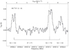 |
Fig. 1 Spectrum of HC17O+ (1−0) at the dust peak of L1544. The hyper-fine structure is shown by vertical solid lines with heights proportional to their relative intensities (see Table 1). The vertical dotted line represents the LSR velocity of L1544 (7.2 km s−1 ). |
Hyperfine transition frequencies measured in the laboratory (Dore et al. 2001), upper energies of HC17O+ (1−0) and relative intensities.
3 Radiative Transfer
In order to fully understand the observed spectra, we need to take into account the transfer of radiation across the source. Physical conditions can vary along the radiation’s path which will affect the observed line intensity and profile. To derive information carried by spectral line profiles, we need to carry out a full radiative transfer modelling of the emission. Radiative transfer accounting for the physical structure of the observed object is crucial for the correct interpretation of spectra, as has been shown in past works, including those on pre-stellar cores (Caselli et al. 2002; Sohn et al. 2007; Keto et al. 2015; Redaelli et al. 2019).
The present work focuses on L1544, a pre-stellar core with well-studied density, temperature and velocity profiles (Ward Thompson et al. 1999; Crapsi et al. 2005, 2007; Keto et al. 2015). In such environments, LTE conditions do not generally apply across the source. In LTE, the energy level populations of molecules are described by the Boltzmann distribution. LTE applies when the critical density of the transition (ncrit = Aul/kul, where Aul is the Einstein A coefficient and kul is the collisional coefficient, where “u” and “l” are the upper and lower levels, respectively) is equal to or lower than the volume density of the emitting region. In pre-stellar cores, volume densities can range from ≳ 106 cm−3 at the centre to ≲ 102 cm−3 at the edge. For example, the CO 1−0 transition has a ncr;t of about 103 cm−3, making LTE not applicable in the outer parts of the core. For transitions with high ncrit, LTE applies only in a small region near the centre of the core. When departing from LTE, collisional rate coefficients are needed to study the transfer of radiation. Furthermore, in non-LTE conditions, the hyperfine component intensity ratio may diverge from statistical weights (e.g. Caselli et al. 1995; Bizzocchi et al. 2013; Faure & Lique 2012; Mullins et al. 2016). In order to accurately predict line intensities resulting from different physical conditions, a full non-LTE radiative transfer treatment with accurate collisional rate coefficients is required.
In Sect. 3.1 we describe the methodology for the hyperfine collisional rate coefficients calculations, in Sect. 3.2 we describe the physical model adopted for L1544 and the LOC radiative transfer code, and in Sect. 3.3 we present the chemical code used to compute the molecular fractional abundance profile.
3.1 Hyperfine Collisional Rate Coefficient Calculations
We determined HC17O+ −H2 rate coefficients from the close coupling (CC) HCO+ −H2 rate coefficients  of Yazidi et al. (2014) using the infinite order sudden (IOS) approximation described in Faure & Lique (2012). We use HCO+ −H2 collisional rate coefficients for HC17O+ as we do not expect a significant difference, as seen in Daniel et al. (2016) where the collisional rate coefficients for N2H+ (isoelectronic of HCO+) and its 15N isotopologues have been found to be similar.
In HC17O+, the coupling between the nuclear spin (I = 5/2) of the 17O atom and the molecular rotation results in a weak splitting (Alexander 1985) of each rotational level J, into hyperfine levels. Each hyperfine level is designated by a quantum number F (F = I + J) varying between ∣I − J∣ and I + J.
Within the IOS approximation, inelastic rotational rate coefficients  can be calculated from the ‘fundamental’ rates (those from the lowest J = 0 level) as follows (Corey & McCourt 1983):
 (1)
(1)
Similarly, IOS rate coefficients among hyperfine structure levels can be obtained from the  rate coefficients using the following formula (Corey & McCourt 1983):
 (2)
(2)
In the above, ( ) and { } are respectively the 3-j and 6-j Wigner symbols.
The IOS approximation, however, is expected to be only moderately accurate at low temperatures. As a result, we compute the hyperfine rate coefficients as (Faure & Lique 2012)
 (3)
(3)
using the CC rate coefficients kCC(0 → L) of Yazidi et al. (2014) for the IOS fundamental rates  in Eqs. (1)−(2).
In addition, we note that the fundamental excitation rates  were replaced by the de-excitation fundamental rates using the detailed balance relation:
 (4)
(4)
This procedure is found to significantly improve the results at low temperature, due to important threshold effects. The calculated rate coefficients can be found in Appendix C.
3.2 The LOC Radiative Transfer Code
Using the radiative transfer code LOC (line transfer with OpenCL; Juvela 2020), we calculate the strength and shape of the HC17O+(1−0) spectrum taking into account its hyperfine structure. The level populations are calculated with the statistical equilibrium equations, which are solved using an accelerated lambda iteration (ALI; Rybicki & Hummer 1991) and the molecule’s radiative and collisional rates. The radiative transfer is calculated using the 1D model in LOC which takes into account the volume density, kinetic temperature, radial velocity, and microturbulence of a spherically symmetric physical structure (see below for pysical parameter ranges).
The physical parameters for the modelling are extracted from a pre-stellar core physical model based on Keto et al. (2015). This 1D model of an unstable quasi-equilibrium Bonnor-Ebert sphere has been shown to be successful in reproducing the profile of several molecular transitions observed towards the dust peak in L1544 (Keto & Rybicki 2010; Keto & Caselli 2010; Caselli et al. 2012, 2017, 2022; Bizzocchi et al. 2013; Redaelli et al. 2018, 2019, Redaelli et al. 2021).
The radial profile of physical properties of the model are plotted in Fig. 2. We note that in order to include these three parameters in this one plot we show the logarithm of the molecular hydrogen number density, the gas temperature divided by 3, and the velocity scaled by −40. The value of n(H2) ranges from 8 × 106 cm−3 at the centre of the core to 1 × 102 cm−3 at the edge of the core (0.32 pc); T ranges from 6 K at the centre of the core to 18 K at the edge; and v ranges from −0.14 km s−1 at the velocity peak (~0.01 pc) to −0.01 km s−1 at the edge of the core.
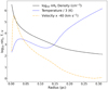 |
Fig. 2 The radial profiles of the Keto et al. (2015) model physical parameters are plotted. The black solid line represents the number density of molecular hydrogen, the blue dashed line the gas temperature, and the orange dash-dotted line the velocity profile of the Keto et al. (2015) physical model. In order to display the various parameters in a single plot, the base 10 logarithm of the number density of molecular hydrogen, the temperature divided by 3, and the velocity scaled by −40 are shown. |
3.3 Chemical Code
The fractional abundance profile of HC17 O+ is simulated using the pseudo-time dependent gas-grain chemical model described in Sipilä et al. (2015). Here we used the same approach to simulate the chemical fractional abundances in L1544 as laid out in Sipilä et al. (2019). Briefly, we adopt the physical model for L1544 of Keto et al. (2015), which is separated into concentric shells; the results of chemical simulations carried out in each shell are combined, yielding time-dependent fractional abundance profiles for the various molecules in the chemical network. The physical structure of the core is thus fixed, while the chemistry evolves in a time-dependent manner. We refer the reader to Sipilä et al. (2015, 2019) for more details on the model, for example the initial fractional abundances. For the present work we extracted several HCO+ fractional abundance profiles in a time interval between 104 and 107 years. The model does not treat oxygen isotope chemistry; to obtain the HC17O+ fractional abundance, we scaled the HCO+ fractional abundance by the isotopic ratio [16O/17O] = 2044 (Penzias 1981; Wilson & Rood 1994). The same procedure was also followed for C17O.
4 Results
4.1 HC17O+
The observed HC17 O+(1−0) can be reproduced by using the prestellar core model and the HC17 O+ fractional abundance profile at 5 × 10⁵ yr with small modifications. The results are shown in the two panels of Fig. 3. The top left panel shows the original model (OM) LOC fit, and the adopted model 1 (AM 1) LOC fit over the observations. The OM histogram is the spectrum LOC produces when using the original pre-stellar core model (from Keto et al. 2015) and the original HC17O+ fractional abundance profile. The AM 1 histogram is the spectrum LOC produces when using the original pre-stellar core model of Keto et al. (2015) and a scaled-up (by a factor of 4) HC17 O+ fractional abundance profile. We use AM 1 to compute the residuals, which can be found in the panel under the spectra. In order to reproduce the intensity of the hyperfine components, we had to scale up the HC17 O+ fractional abundance profile by a factor of 4. However, this model fails to reproduce the double-peak morphology of the lines and for this a further change is needed.
The top right panel of Fig. 3 shows (solid red histogram) a different adopted model 2 (AM 2) LOC fit overlaid on the observations (in black). The AM 2 corresponds to AM 1 with a scaled-up (by 30%, ranging from −0.4 at the velocity peak to −0.01 km s−1 at the edge of the core) velocity profile instead of the velocity profile from the pre-stellar core physical model of Keto et al. (2015). We use the AM 2 to compute the residuals, which can be found in the panel under the spectra. There is a reduction of the residual standard deviation of 0.7 mK compared to the AM 1 in the left panel, which only takes into account the HC17O+ fractional abundance profile scaling. The reasons behind the adjustments of the original pre-stellar core model is discussed in Sect. 5.
Using the HC17O+ fractional abundance profile in the adopted models of Fig. 3 and the physical structure given in input to LOC, we can derive the column density of HC17O+. This is done by integrating the multiplication of the fractional abundance profile (see Fig. 4) by the gas density and convolving to the beam size (28″). The column density derived from the fractional abundance profile used to model the observations in Fig. 3 is  cm−2. The column density uncertainty is derived with the approach used in Redaelli et al. (2018). We compute several models from scaled fractional abundance profiles, from which we derive the corresponding column density values. The χ2 values are derived from the comparison of these models with the observations. We then plot χ2 versus the column density values. The column density uncertainties are derived setting a χ2 upper and lower limits to 15%. The excitation temperature computed by LOC for the three HC17O+(1−0) hyperfine transitions throughout the core is plotted in Fig. 5 in black. We can see that the Tex profiles of the different hyperfine components do not vary significantly. In order to compare this method with the column density calculation from the line fitting with Gaussians in a CTex (constant Tex) approximation (see Caselli et al. 2002), we perform hyperfine structure (HFS) fits in CLASS. Next, assuming an excitation temperature of 5 K, we calculate a HC17 O+ column density of 4.1 ± 0.3 × 1010 cm−2. The choice for Tex comes from N2H+ (1−0), which has a similar critical density to HC17O+(1−0) (1.4 × 10⁵ and 1.5 × 105 cm−3, respectively), observed towards L1544 in Crapsi et al. (2005). For this calculation we use the optically thin approximation as we have confirmed the HC17O+ J =1−0 transition to be optically thin (details of the calculation can be found in Appendix B). The column density derived with the simple CTex method is in agreement within the errors with the value derived with our model. Furthermore, we compare these two column density values with that obtained by scaling the HC18O+ column density derived in Redaelli et al. (2019) by [18O/17O] = 3.67, yielding a HC17O+ column density of 4.6 ± 0.3 × 1010 cm−2.
4.2 C17O
The J = 1−0 transition of C17O has been observed towards L1544 by Chacón-Tanarro et al. (2019). Contrary to HC17O+, C17O presents single-peaked hyperfine components, even though it is also an optically thin transition. The critical densities of HC17O+(1−0) and C17O(1−0) are 1.5 × 105 cm−3 and 2.0 × 103 cm−3, respectively, as calculated from the Einstein and collisional coefficients at 10 K from the Leiden Atomic and Molecular Database (LAMDA)2. To model the hyperfine C17O emission the hyperfine collisional rate coefficients were required, which we approximated from the non-hyperfine collisional rate coefficients available at LAMDA (Yang et al. 2010) with a M j randomisation approach (Appendix D). We note that Dagdigian (2022) has recently also computed hyperfine C17 O collisional rate coefficients using the recoupling technique. As in the case of HC17O+, we are able to reproduce the observed spectrum with the pre-stellar core model detailed in Sect. 3.2, and the fractional abundance profile at 5 × 10⁵ yr described in Sect. 3.3 with a scaling factor of 3. Results are shown in the two panels of Fig. 6. The top left panel shows the OM LOC fit, and the AM 1 LOC fit over the observations. The OM histogram is the spectrum LOC produces with the original pre-stellar core model and original C17O fractional abundance profile. The AM 1 histogram is the spectrum LOC produces with the original pre-stellar core model and an fractional abundance profile of C17O scaled up by a factor of 3, needed to fit the intensity of the observed lines (similar to those found in the case of HC17O+). The AM 1 is the model we use to compute the residuals, which can be found in the panel under the spectra. They show an overall good agreement between the AM 1 and the observations.
The top right panel of Fig. 6 shows the AM 2 LOC spectrum overlaid on the observations. The AM 2 corresponds to the AM 1 with a velocity profile scaled up by 30% (ranging from -0.4 at the velocity peak to −0.01 km s−1 at the edge of the core). We use the AM 2 to compute the residuals, which can be found in the panel under the spectra. The right bottom panel shows the residuals obtained by subtracting the observed spectrum from the AM 2 spectrum. Contrarily to HC17O+, there is an increase in the residual standard deviation of 1.5 mK when a scaled-up velocity profile is adopted. Therefore, the best model for reproducing the C17O observed spectrum is the one that uses the increased (by a factor of 3) C17O fractional abundance profile and the original pre-stellar core velocity profile (AM 1 in the upper left panel of Fig. 6). The reason behind this difference between HC17O+(1−0) and C17O(1−0) observations is discussed in Sect. 5.
We have also computed the C17O column density from the fractional abundance profile used in LOC to fit the observations as done with HC17O+. The excitation temperature computed by LOC for the three C17O(1−0) hyperfine transitions throughout the core is plotted in Fig. 5 in blue. The Tex profiles of the different hyperfine components do not vary significantly from each other. The calculated C17O column density is  cm−2 (the uncertainty is calculated in the same way as for HC17O+). The column density calculated in Chacón-Tanarro et al. (2019) is 6.8 ± 0.6 × 1014 cm−2, 41% higher than the column density extracted from the C17O fractional abundance profile used for the modelling with LOC. This difference in column densities could be due to the Tex used; Chacón-Tanarro et al. (2019) assume a constant Tex of 10 K across the core, while LOC computes the column density using the Tex radial profile (Fig. 5).
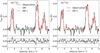 |
Fig. 3 The results of the HC17O+ observed spectrum modelling with LOC are displayed. Left: observed spectrum of the HC17O+ (1−0) (black), the result of a simulation using the original HC17O+ fractional abundance profile at 5 × 10⁵ yr and the original pre-stellar core model (OM; dotted red) and the result of a simulation using the HC17O+ fractional abundance profile at 5 × 10⁵ yr upscaled by a factor of 4 times that of the original pre-stellar core model (AM 1; solid red). Residuals are computed with the adopted model and are shown in the lower panel. The dashed lines represent the 3σ levels. Right: observed spectrum of the HC17O+ (1−0) (black) and the result of a simulation using the HC17O+ fractional abundance profile at 5 × 10⁵ yr upscaled by a factor of 4 and an upscaled velocity profile by 30% (AM 2; solid red). Residuals are computed with the adopted model and are shown in the lower panel. The dashed lines represent the 3σ levels. |
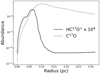 |
Fig. 4 Comparison between the HC17O+ and C17O radial abundance profiles. The dotted curve shows the C17O fractional abundance (abundance with respect to H2) as a function of radius. The solid curve shows the fractional abundance of HC17O+, scaled by 104 computed with the chemical code from Sipilä et al. (2015, 2019) by scaling the CO and HCO+ fractional abundance profiles by the isotope ratio [16O/17O] = 2044 (Penzias 1981; Wilson & Rood 1994). |
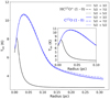 |
Fig. 5 Excitation temperature profile of the three HC17O+(1−0) and C17O(1−0) hyperfine transitions across the core. The HC17O+(1−0) 5/2 → 3/2, 5/2 → 7/2, and 5/2 → 5/2 transitions are plotted as a black solid line, a black dash-dotted line, and a black dotted line, respectively. The profiles for HC17O+ are superimposed. The C17O(1−0) 5/2 → 3/2, 5/2 → 7/2, and 5/2 → 5/2 transitions are plotted as a blue solid line, a blue dash-dotted line, and a blue dotted line, respectively. The inset presents a zoom-in of the radial Tex profile from 0 to 0.1 pc. |
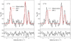 |
Fig. 6 The results of the C17O observed spectrum modelling with LOC are displayed. Left: observed spectrum of the C17O (1−0) (black). This spectrum is the result of a simulation using the original C17O fractional abundance profile at 5 × 10⁵ yr and the original pre-stellar core model (OM; dotted red) and the result of a simulation using the C17O fractional abundance profile at 5 × 10⁵ yr upscaled by a factor of 3 and the original pre-stellar core model (AM 1; solid red). The residuals are computed with the adopted model, and are shown in the lower panel. The dashed lines represent the 3σ levels. Right: observed spectrum of the C17O (1−0) (black) and the result of a simulation using the C17O fractional abundance profile at 5 × 10⁵ yr increased by a factor of 3 and a scaled-up velocity profile by 30% (AM 2; solid red). Residuals are computed with the adopted model and are shown in the lower panel. The dashed lines represent the 3σ levels. |
5 Discussion
In past works two scenarios have been discussed to explain the double-peaked morphology in optically thin transitions observed towards L1544 (Tafalla et al. 1998; Caselli et al. 2002): the presence of two velocity components in the line of sight and the depletion of the molecules towards the centre of the core.
The double-peaked structure of the optically thin C34S (2−1) line is thought to arise from two separate velocity components on the line of sight at 7.10 and 7.25 km s−1 that overlap in the centre (Tafalla et al. 1998). We discard the two velocity component scenario for our case as this would produce double-peaked lines also from C17O(1−0), in disagreement with observations, as shown in Fig. 6. Moreover, we are able to reproduce the HC17O+(1−0) line profile using a simple model of an individual object in contraction, as also found in the past using other molecular lines.
In Caselli et al. (2002) it is suggested that the optically thin double-peaked line profiles of the F1, F = 1,0 → 1,1 line of N2H+ (1−0) and HC18O+ (1−0) towards L1544 arise from the depletion of these molecules towards the centre of the core. To mimic this depletion the fractional abundances of N2H+ and HC18O+ were set to 0 between the centre and 2000 and 1400 au, respectively. The size of these gaps in the fractional abundance profiles are related to the radius from the centre of the core at which these molecules present significant depletion. This artificial depletion reproduced the F1, F = 1,0 → 1,1 line of N2H+ (1−0) and HC18O+ (1−0) line profiles. To test whether an enhanced depletion of HC17O+ towards the core centre would reproduce the observations, we created a ‘hole’ in the fractional abundance profile, similarly to Caselli et al. (2002; more information in Appendix A.1), but the central depletion of HC17O+ does not reproduce the observed line profile (e.g. Fig. A.1). This was expected as the chemical model already naturally predicts the depletion of HCO+ towards the central part of the core.
Self-absorption is not expected to produce double peaks in lines of low abundance species, as their concentration in the low-density foreground layer is not large enough to absorb photons emitted in the dense core. Nevertheless, self-absorption has been considered as a possible contribution to double-peaked line morphologies for some transitions in past works (Caselli et al. 1999, 2002). To make sure that a sufficient concentration of HC17O+ in a foreground layer would not induce self absorption, we modelled the observations by adding an profile from 0.3 to 1.5 pc with a HC17O+ layer corresponding to a visual extinction of Av = 4 mag (more information in the Appendix A.2). This test also did not reproduce the observed spectrum, as shown in Fig. A.2.
One of the parameters that improved the fitting of lines in L1544 in past works is the velocity profile. In Bizzocchi et al. (2013), upscaling the velocity profile by 75% was necessary to reproduce the high-sensitivity observations of N2H+(1−0) towards L1544. Both the observed linewidth and line profiles are well reproduced with LOC using a constant alongside the upscaled velocity profile from the Keto & Caselli (2008) physical structure model (Fig. 5 in Bizzocchi et al. 2013). The upscaling of the velocity profile allows the further splitting in velocity of the two contracting parts of the cloud lying in front and behind the core centre where the density is close to the critical density of the transition (1.5 × 105 cm−3). As in Bizzocchi et al. (2013), in our case this is reflected in the split of the HC17O+(1−0) hyperfine components in agreement with the observed spectrum shown in Fig. 1.
Infall motions were also invoked to explain the double-peaked profiles of HC18O+ 1−0 and N2H+ 1−0 towards the dust peak of L1544 in van der Tak et al. (2005). HC18O+ presents a line split where the two peaks appear with the same intensity, while N2H+ presents the well-known blue asymmetry in the peak intensity indicating that the line is self-absorbed. In this paper they combine the core physical model from Galli et al. (2002) with infall models at the t3 and t5 time steps from Ciolek & Basu (2000), which correspond respectively to 2.660 and 2.684 Myr after the start of the core collapse. Nevertheless, this model was not able to reproduce the H2D+ 110 − 111 spectral line profile. In our work we used a physical core model (Keto & Caselli 2010) which was tailored specifically for L1544, and includes infall dynamics which are consistent with the physical structure, as well as a state-of-the-art chemical model (Sipilä et al. 2015). Our model reproduced a great number of molecular lines (see Sect. 3.2) including HC18O+ (1−0) and N2H+ (1−0) in Redaelli et al. (2019). Moreover, the higher spectral resolution (by 0.02 km s−1) of our HC17O+ (1−0) spectrum and the hyperfine splitting allows us to refine the physical model by fitting the line profile, compared to previous HC18O+ (1−0) observations. The velocity profiles used in van der Tak et al. (2005) range for t3 and t5 are respectively from −0.01 to −0.14 and −0.01 to −0.19 km s−1 (see Fig. 2 in Ciolek & Basu 2000). These velocity profiles differ from the one we used to model HC17O+, where the velocity peak has an average of 2.5 times higher velocity than the maximum velocity in the profiles used for the modelling in van der Tak et al. (2005).
The different line profiles of HC17O+(1−0) and C17O(1−0) arise from their different critical densities and spatial distributions in the core. HC17O+ and C17O have different critical densities (1.5 × 105 cm−3 and 2.0 × 103 cm−3, respectively). The profile and critical density combination causes the HC17O+ line to emit preferentially closer to the core centre (see its excitation temperature profile in Fig. 5, in black), while C17O has a more extended emission (see its excitation temperature profile in Fig. 5, in blue). As HC17O+ emits in a small region close to the centre, where the contraction velocity also has a peak, the spectrum results in a double peak, where the local contraction velocity is 30% higher than in the original model of Keto et al. (2015). Unlike HC17O+, the C17O emission arises from lower density gas further away from the core centre where the contraction velocity is lower (see Fig. 2), resulting in a single peak. The fact that an upscaled velocity profile fits the HC17O+(1−0) line profile but not C17O simply tells us that the infall velocity is higher towards the inner part of the core, as expected in a contracting Bonnor–Ebert sphere (Keto & Rybicki 2010) at a more evolved stage compared to the one adopted by Keto et al. (2015). We estimate that it would take an additional 1 × 10⁴ yr for the infall velocity peak to increase by 30%. We also note that L1544 is not spherically symmetric, as assumed so far, but has an elongated structure (Caselli et al. 2002). More complex simulations have been done taking into account a flattened structure for L1544, which more closely resembles reality (Caselli et al. 2019). Nevertheless, Caselli et al. (2022) show that the density and velocity profiles along the major and minor axes of the 3D simulation are very close to the same profiles in the spherically symmetric model of Keto et al. (2014), reinforcing the accuracy of the Keto et al. (2015) model, despite its simplicity. The need to take into account the physical structure and kinematics of a source when interpreting its spectra is made evident in this work. Using a slab model that does not take into account the physical or the kinematic structure of the core can lead to the derivation of non-accurate parameters and, in this case, does not allow us to reach any conclusions about the nature of the physical process behind the double-peaked profiles. As we show in Sect. 4, the HC17O+ and C17O models both required an upscaling of the fractional abundance profile used to fit the observations. The necessary HC17O+ fractional abundance adjustment required to fit the observations is done by adjusting the HCO+ profile predicted by our chemical code (see Sect. 3.3). We note that the HCO+ fractional abundance profile resulting from a static model, where the physical structure is kept fixed while the chemistry is evolving, differs from the profile computed with a dynamic model, as can be seen in the central upper panel in Fig. 12 in Sipilä & Caselli (2018). The fractional abundance profile of HCO+ in the static model appears approximately three times higher than the profile obtained with the dynamic model at the very centre of the core (until 2.0 × 10⁴ au) and about four times lower from 2.0 104 to 2.5 × 10⁴ au. However, the physical model discussed in Sipilä & Caselli (2018) refers to a dense core with a mass of 7.2 M⊙ which is significantly lower than that of L1544 described by Keto & Caselli (2010) (10 M⊙), so the dynamic model results cannot be used here. We are currently preparing a new dynamical model for L1544 that will help to constrain the issue of static versus dynamic models (Sipilä et al. 2022). Finally, the fact that the fractional abundances of HC17O+ and C17O needed to be upscaled by a similar factor can be the consequence of too large CO depletion compared to the observations, also suggesting that dynamics could help in better reproducing our data (as less CO-depleted material keeps moving towards the central regions, unlike in the static model).
6 Conclusions
In this article we have presented new high-sensitivity and highresolution HC17O+ J = 1−0 observations towards the dust peak of L1544, which has revealed the double-peaked nature of its hyperfine components. By carrying out a full non-LTE radiative transfer modelling of HC17O+(1−0) with new hyperfine collisional rate coefficients, we have explored what is causing the double-peaked profile observed in optically thin transitions of high-density tracers. The power of fully taking into account radiative transfer is made evident in this work where a modelling of the entire source is needed to reproduce the observed line profile. Moreover, we have tested the model by reproducing previous observations of the C17O(1−0) line, which presents a single-peaked line morphology. Our main conclusions are as follows:
The HC17O+(1−0) line profile can be reproduced with a model of a contracting pre-stellar core; there is no evidence for separate velocity components along the line of sight. This indicates that a double-peaked profile towards a centrally condensed core can be solely an effect of radiative transfer in a contracting centrally concentrated dense core. In the present work the reason for the double peak lies in the infall velocity and the critical density of the line. This makes the line sensitive to the motions at radii of about 0.01 pc where the volume density is close to the critical density, and the contraction velocity has a peak.
The fact that an upscaled velocity profile was required to reproduce HC17O+ but not C17O suggests that the L1544 pre-stellar core is more dynamically evolved than previously thought (1 × 10⁴ yr), as higher velocities (30% higher than the original physical model) are required towards the core centre to reproduce the splitting. Higher central velocities are in fact expected in contracting BE spheres at later stages of evolution (Keto & Caselli 2010).
Both the HC17O+ and C17O fractional abundances are underproduced by our chemical models by a factor of 4 and 3 respectively. This suggests that predicted CO freeze-out is too large, possibly due to the physical model not evolving dynamically.
Line profiles are shown to be powerful tools to gain insight on the physical, chemical, and kinematic structure of pre-stellar cores. In the future we will build upon the results of this manuscript with the study of complementary transition line profiles towards L1544.
Acknowledgements
J.F.A., S.S., P.C., F.O.A., O.S, E.R. and L.B. gratefully acknowledge the support of the Max Planck Society.
Appendix A Results of the Considered Scenarios
In this section we present complementary results obtained to evaluate the viability of the different possible scenarios for the HC17O+(1−0) double-peaked structure. All the models presented were computed with a HCO+ fractional abundance profile at t = 5 × 10⁵ yr, and thus are comparable with the best-fit results (AM 2 in Figure 3). Fractional abundance profiles at time steps between 104 and 107 yr were also tested, and lead to less accurate fits with larger residual standard deviations.
A.1 Depletion
The chemical model takes into account the CO depletion by freeze-out at the centre of the core. This affects the HCO+ fractional abundance (Figure 4) as this molecule is formed by the reaction of CO with  . Following the idea that the model flat-topped profiles in the OM of Figure 3 could be the result of the enhanced HC17O+ depletion towards the core centre, we tested larger depletions than those taken into account in the chemical model to see whether we could fit the observed line profiles better. To this end, we modelled the radiative transfer of the molecule with a modified fractional abundance profile creating fractional abundance holes with different radii. We tested the effect of a 7000 au radius hole, and show the resulting spectra from a model with HC17O+ depletion from 0 to 7000 au in Figure A.1. We note that in order to distinguish the feature of the lines properly, the HC17O+ fractional abundance had to be increased by a factor of 16 to make the spectrum visible in the figure. We obtain a faint line emission with a double-peaked feature, which is not enhanced from the OM profile in Figure 3. Therefore, the HC17O+ depletion towards the centre of the core alone cannot explain the observed double-peaked structure.
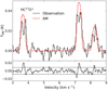 |
Fig. A.1 Spectrum of the HC17O+ (1−0) observation (black) and product of model with the upscaled by a factor of 16 fractional abundance profile at 5 × 10⁵ yrs and modified to have 0 fractional abundance from 0 to 7000 au (red). |
A.2 Self-Absorption
Self-absorption is not expected for an optically thin transition such as HC17O+(1−0). Nevertheless, we tested the effects of an envelope-like extension added to the fractional abundance profile corresponding to a visual extinction of Av = 4 mag, which lengthens the fractional abundance profile from 0.3 to 1.7 pc. In Figure A.2 we present the Av = 4 mag extended model spectrum with a HC17O+ fractional abundance profile scaled up by a factor of 3 to be able to distinguish possible self-absorption features in the line profiles. This trial does not show signs of HC17O+ (1−0) self-absorption nor does it reproduce the observed line profile, which gives evidence that an enhanced HC17O+ molecular fractional abundance in the foreground does not account for the observed line shape.
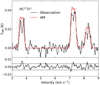 |
Fig. A.2 Spectrum of the HC17O+ (1−0) observation (black) and product of model with an upscaled by a factor of 3 extended fractional abundance profile with Av = 4 at 5 × 10⁵ yrs. |
Appendix B Comparison with Constant Tex (CTex) Approximation
To derive the column density from the observations we first checked that the HC17O+(1−0) transition is optically thin. A first fit with CLASS returns larger optical depth uncertainties than optical depth values. In the optically thin approximation (τv<0.1, where τv represents the total optical depth) τv is not included in the radiative transfer equation, and thus the problem degenerates, resulting in the large optical depth uncertainties observed. As the optical depth derivation for this case with CLASS is not possible, we estimate its value with the following equation, assuming three different Tex values (5, 7 and 9 K):
![Mathematical equation: $ {\tau _v} = - ln\left[ {1 - {{{T_{{\rm{MB}}}}} \over {\left[ {{J_v}\left( {{T_{ex}}} \right) - {J_v}\left( {{T_{bg}}} \right)} \right]}}} \right]. $](/articles/aa/full_html/2022/11/aa43927-22/aa43927-22-eq16.png) (B-1)
(B-1)
The total optical depth is represented by τv, and the line brightness temperature by TMB ; Jv(Tex) and Jv(Tbg) correspond to the Rayleigh-Jeans equivalent temperature at Tex and Tbg, respectively. The optical depth obtained for the line lies between 0.03 and 0.08, which confirms that the J = 1−0 rotational transition of HC17O+ is optically thin.
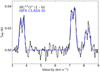 |
Fig. B.1 Spectrum of the HC17O+ J = 1 − 0 at the dust peak of L1544 (black). The HFS fit was done with CLASS (blue). |
Results of the class HFS fit of the observed HC17O+(1−0) rotational transition towards L1544, treating the two peaks of each hyperfine line as separate velocity components.
We then proceed to fit the observations with the hyperfine structure (HFS) tool in class. This tool fits the hyperfine components of a transition using laboratory calculated frequencies, assuming a Gaussian velocity distribution, the same excitation temperature of the hyperfine components, and local standard of rest (LSR) velocity. In our particular case we also fixed the optical depth to the minimum value allowed (0.1) to indicate that the line is optically thin. In order to reproduce the double peak, as kinematic information cannot be included in CLASS, we applied this tool taking into account two separate velocity components. This fit results in a hyperfine component model that follows the statistical intensity ratios. In non-CTex conditions, the relative intensity amongst hyperfine components can differ from the statistical value. In our case, however, the ratio of intensities does not differ significantly from the statistical values.
With the parameters derived from HFS fittings (Table B.1) and the HC17O+ molecular constants extracted from the Cologne Database for Molecular Spectroscopy (CDMS)3, we calculated the column density of the molecule assuming that the transition is optically thin. For this purpose, we use Equation B.2 (Mangum & Shirley 2015),
Derived column densities from HFS fitting.
 (B.2)
(B.2)
where NTOT is the total column density, kB is the Boltzmann constant, ν is the transition frequency, Aul is the Einstein coefficient, h is the Planck constant, c is the light speed, Eu is the upper level energy, and W is the integrated intensity. As seen in Table B.1, the HFS fit returns, for each velocity component, the summed TMB of the three hyperfine lines and the average linewidth Δv. We calculated a global W for each velocity component from the TMB and Δv assuming a Gaussian profile. In Equation B.2, gu represents the combined upper level degeneracy of the hyperfine transitions, which equals 18. Lastly, Qrot represents the partition function. We used three different Qrot values, 16.54, 22.23, and 27.94, for three different Tex values, 5, 7, and 9 K, used for the calculations. The result is six column density values, corresponding to two velocity components and three assumed Tex (Table B.2).
The column density of the two fitted velocity components are then summed for each Tex resulting in the calculated total HC17O+ column density. The derived total column densities are the same for all Tex within the uncertainties. We conclude that the column densities do not strongly depend on the Tex used in the range of values considered here. The derived column density of HC17O+ at Tex = 5K towards L1544 is 4.1±0.3 × 1010 cm−2. On the other hand, the extracted column density from the HC17O+ fractional abundance profile used to fit the observational spectrum with LOC is  cm−2, consistent within the errors with the column density obtained with CLASS. Contrary to a CTex approach where a single excitation temperature is used, the column density derivation from the fractional abundance profile integration takes into account the excitation temperature profile across the core (Figure 5).
Appendix C HC17O+ Hyperfine Collisional Rate Coefficients
In this section we present for the first time the HC17O+ −H2 hyperfine collisional rate coefficients calculated with the method described in Section 3.1. For each transition J, F → J′, F′, where the J′ and F′ quantum numbers refer to the final energy levels and J and F indicate the initial energy levels, collisional coefficient values in units of cm3 s−1 are given for five temperatures: 10, 20, 30, 40, and 50 K (Table C.1).
HC17O+ hyperfine collisonal rate coefficients given in units of cm3 s−1 for 10, 20, 30, 40, and 50 K. Transitions are labelled with the J, F → J′ ,F′ quantum numbers, where the J′ and F′ quantum numbers refer to the final energy levels and J and F indicate initial energy levels.
Appendix D C17O Hyperfine Collisional Rate Coefficients
We approximated the C17O-H2 hyperfine collisional rate coefficients from the non-hyperfine collisional rate coefficients available in LAMDA using the Mj-randomisation method (Franz & Franz 1966). For each transition J, F → J′, F′, where the J′ and F′ quantum numbers refer to the final energy levels and J and F indicate initial energy levels, collisional coefficient values with units of cm3 s−1 are given for seven temperatures: 2, 5, 10, 20, 30, 40, and 50 K (Table D.1).
C17O hyperfine collisonal rate coefficients given in units of cm3 s−1 for 2, 5, 10, 20, 30, 40, and 50 K. Transitions are labelled with the J, F → J′ ,F′ quantum numbers, where the J′ and F′ quantum numbers refer to the final energy levels and J′ and F′ indicate the initial energy levels.
References
- Alexander, M. H. 1985, Chem. Phys., 92, 337 [NASA ADS] [CrossRef] [Google Scholar]
- André, P., Di Francesco, J., Ward-Thompson, D., et al. 2014, in Protostars and Planets VI, eds. H. Beuther, R. S. Klessen, C. P. Dullemond, & T. Henning (Tucson: University of Arizona Press), 27 [Google Scholar]
- Bizzocchi, L., Caselli, P., Leonardo, E., & Dore, L. 2013, A&A, 555, A109 [NASA ADS] [CrossRef] [EDP Sciences] [Google Scholar]
- Caselli, P., Myers, P., & Thaddeus, P. 1995, ApJ, 455, L77 [NASA ADS] [CrossRef] [Google Scholar]
- Caselli, P., Walmsley, C., Tafalla, M., Dore, L., & Myers, P. 1999, ApJ, 523, L165 [NASA ADS] [CrossRef] [Google Scholar]
- Caselli, P., Walmsley, C., Zucconi, A., et al. 2002, ApJ, 565, 331 [NASA ADS] [CrossRef] [Google Scholar]
- Caselli, P., Keto, E., Bergin, E., et al. 2012, ApJ, 759, L37 [NASA ADS] [CrossRef] [Google Scholar]
- Caselli, P., Bizzocchi, L., Keto, E., et al. 2017, A&A, 603, L1 [NASA ADS] [CrossRef] [EDP Sciences] [Google Scholar]
- Caselli, P., Pineda, J., Zhao, B., et al. 2019, ApJ, 874, 89 [NASA ADS] [CrossRef] [Google Scholar]
- Caselli, P., Pineda, J. E., Sipilä, O., et al. 2022, ApJ, 929, 13 [NASA ADS] [CrossRef] [Google Scholar]
- Chacón-Tanarro, A., Caselli, P., Bizzocchi, L., et al. 2019, A&A, 622, A141 [Google Scholar]
- Ciolek, G. E., & Basu, S. 2000, ApJ, 529, 925 [Google Scholar]
- Corey, G. C., & McCourt, F. R. 1983, J. Phys. Chem, 87, 2723 [CrossRef] [Google Scholar]
- Crapsi, A., Caselli, P., Walmsley, C. M., et al. 2005, ApJ, 619, 379 [Google Scholar]
- Crapsi, A., Caselli, P., Malcolm, C., & Tafalla, M. 2007, A&A, 470, 221 [NASA ADS] [CrossRef] [EDP Sciences] [Google Scholar]
- Dagdigian, P. J. 2022, MNRAS, 514, 2214 [NASA ADS] [CrossRef] [Google Scholar]
- Daniel, F., Faure, A., Pagani, L., et al. 2016, A&A, 592, A45 [NASA ADS] [CrossRef] [EDP Sciences] [Google Scholar]
- Dore, L., Cazzoli, G., & Caselli, P. 2001, A&A, 368, 721 [Google Scholar]
- Faure, A., & Lique, F. 2012, MNRAS, 425, 740 [NASA ADS] [CrossRef] [Google Scholar]
- Franz, F. A., & Franz, J. R. 1966, Phys. Rev., 148, 82 [NASA ADS] [CrossRef] [Google Scholar]
- Galli, D., Walmsley, M., & Gonçalves, J. 2002, A&A, 394, 275 [NASA ADS] [CrossRef] [EDP Sciences] [Google Scholar]
- Galli, P. A. B., Loinard, L., Bouy, H., et al. 2019, A&A, 630, A137 [NASA ADS] [CrossRef] [EDP Sciences] [Google Scholar]
- Guélin, M., Cernicharo, J., & Linke, R. 1982, ApJ, 263, L89 [CrossRef] [Google Scholar]
- Jiménez-Serra, I., Vasyunin, A. I., Caselli, P., et al. 2016, ApJ, 830, L6 [Google Scholar]
- Jin, M., & Garrod, R. T. 2020, ApJS, 249, 26 [Google Scholar]
- Juvela, M. 2020, A&A, 644, A151 [NASA ADS] [CrossRef] [EDP Sciences] [Google Scholar]
- Keto, E., & Caselli, P. 2008, ApJ, 683, 238 [Google Scholar]
- Keto, E., & Caselli, P. 2010, MNRAS, 402, 1625 [Google Scholar]
- Keto, E., & Rybicki, G. 2010, ApJ, 716, 1315 [NASA ADS] [CrossRef] [Google Scholar]
- Keto, E., Rawlings, J., & Caselli, P. 2014, MNRAS, 440, 2616 [NASA ADS] [CrossRef] [Google Scholar]
- Keto, E., Caselli, P., & Rawlings, J. 2015, MNRAS, 446, 3713 [Google Scholar]
- Lique, F., Daniel, F., Pagani, L., & Feautrier, N. 2015, MNRAS, 446, 1245 [NASA ADS] [CrossRef] [Google Scholar]
- Mangum, J. G., & Shirley, Y. L. 2015, PASP, 127, 266 [Google Scholar]
- Mullins, A. M., Loughnane, R. M., Redman, M. P., et al. 2016, MNRAS, 459, 2882 [Google Scholar]
- Penzias, A. 1981, ApJ, 249, 518 [NASA ADS] [CrossRef] [Google Scholar]
- Pety, J. 2005, in SF2A-2005: Semaine de l’Astrophysique Francaise, ed. F. Casoli, T. Contini, J. M. Hameury, & L. Pagani, 721 [Google Scholar]
- Redaelli, E., Bizzocchi, L., Caselli, P., et al. 2018, A&A, 617, A7 [NASA ADS] [CrossRef] [EDP Sciences] [Google Scholar]
- Redaelli, E., Bizzocchi, L., Caselli, P., et al. 2019, A&A, 629, A15 [NASA ADS] [CrossRef] [EDP Sciences] [Google Scholar]
- Redaelli, E., Sipilä, O., Padovani, M., et al. 2021, A&A, 656, A109 [NASA ADS] [CrossRef] [EDP Sciences] [Google Scholar]
- Rybicki, G., & Hummer, D. 1991, A&A, 245, 171 [NASA ADS] [Google Scholar]
- Sipilä, O., & Caselli, P. 2018, A&A, 615, A15 [Google Scholar]
- Sipilä, O., Caselli, P., & Harju, J. 2015, A&A, 578, A55 [Google Scholar]
- Sipilä, O., Caselli, P., Redaelli, E., Juvela, M., & Bizzocchi, L. 2019, MNRAS, 487, 1269 [Google Scholar]
- Sipilä, O., Caselli, P., Redaelli, E., & Spezzano, S. 2022, A&A, in press, https://doi.org/10.1051/0004-6361/202243935 [Google Scholar]
- Sohn, J., Lee, C. W., Park, Y.-S., et al. 2007, ApJ, 664, 928 [NASA ADS] [CrossRef] [Google Scholar]
- Spezzano, S., Caselli, P., Bizzocchi, L., Giuliano, B. M., & Lattanzi, V. 2017, A&A, 606, A82 [NASA ADS] [CrossRef] [EDP Sciences] [Google Scholar]
- Tafalla, M., Mardones, D., Myers, P., et al. 1998, ApJ, 504, 900 [NASA ADS] [CrossRef] [Google Scholar]
- van der Tak, F. F. S., Caselli, P., & Ceccarelli, C. 2005, A&A, 439, 195 [NASA ADS] [CrossRef] [EDP Sciences] [Google Scholar]
- Vastel, C., Ceccarelli, C., Lefloch, B., & Bachiller, R. 2014, ApJ, 795, L2 [NASA ADS] [CrossRef] [Google Scholar]
- Ward-Thompson, D., Motte, F., & Andre, P. 1999, MNRAS, 305, 143 [Google Scholar]
- Williams, J., Rohrbacher, A., Seong, J., et al. 1999, J. Chem. Phys., 111, 997 [NASA ADS] [CrossRef] [Google Scholar]
- Wilson, T., & Rood, R. 1994, ARA&A, 32, 191 [CrossRef] [Google Scholar]
- Yang, B., Stancil, P. C., Balakrishnan, N., & Forrey, R. C. 2010, ApJ, 718, 1062 [Google Scholar]
- Yazidi, O., Ben Abdallah, D., & Lique, F. 2014, MNRAS, 441, 664 [NASA ADS] [CrossRef] [Google Scholar]
All Tables
Hyperfine transition frequencies measured in the laboratory (Dore et al. 2001), upper energies of HC17O+ (1−0) and relative intensities.
Results of the class HFS fit of the observed HC17O+(1−0) rotational transition towards L1544, treating the two peaks of each hyperfine line as separate velocity components.
HC17O+ hyperfine collisonal rate coefficients given in units of cm3 s−1 for 10, 20, 30, 40, and 50 K. Transitions are labelled with the J, F → J′ ,F′ quantum numbers, where the J′ and F′ quantum numbers refer to the final energy levels and J and F indicate initial energy levels.
C17O hyperfine collisonal rate coefficients given in units of cm3 s−1 for 2, 5, 10, 20, 30, 40, and 50 K. Transitions are labelled with the J, F → J′ ,F′ quantum numbers, where the J′ and F′ quantum numbers refer to the final energy levels and J′ and F′ indicate the initial energy levels.
All Figures
|
Fig. 1 Spectrum of HC17O+ (1−0) at the dust peak of L1544. The hyper-fine structure is shown by vertical solid lines with heights proportional to their relative intensities (see Table 1). The vertical dotted line represents the LSR velocity of L1544 (7.2 km s−1 ). |
| In the text | |
|
Fig. 2 The radial profiles of the Keto et al. (2015) model physical parameters are plotted. The black solid line represents the number density of molecular hydrogen, the blue dashed line the gas temperature, and the orange dash-dotted line the velocity profile of the Keto et al. (2015) physical model. In order to display the various parameters in a single plot, the base 10 logarithm of the number density of molecular hydrogen, the temperature divided by 3, and the velocity scaled by −40 are shown. |
| In the text | |
|
Fig. 3 The results of the HC17O+ observed spectrum modelling with LOC are displayed. Left: observed spectrum of the HC17O+ (1−0) (black), the result of a simulation using the original HC17O+ fractional abundance profile at 5 × 10⁵ yr and the original pre-stellar core model (OM; dotted red) and the result of a simulation using the HC17O+ fractional abundance profile at 5 × 10⁵ yr upscaled by a factor of 4 times that of the original pre-stellar core model (AM 1; solid red). Residuals are computed with the adopted model and are shown in the lower panel. The dashed lines represent the 3σ levels. Right: observed spectrum of the HC17O+ (1−0) (black) and the result of a simulation using the HC17O+ fractional abundance profile at 5 × 10⁵ yr upscaled by a factor of 4 and an upscaled velocity profile by 30% (AM 2; solid red). Residuals are computed with the adopted model and are shown in the lower panel. The dashed lines represent the 3σ levels. |
| In the text | |
|
Fig. 4 Comparison between the HC17O+ and C17O radial abundance profiles. The dotted curve shows the C17O fractional abundance (abundance with respect to H2) as a function of radius. The solid curve shows the fractional abundance of HC17O+, scaled by 104 computed with the chemical code from Sipilä et al. (2015, 2019) by scaling the CO and HCO+ fractional abundance profiles by the isotope ratio [16O/17O] = 2044 (Penzias 1981; Wilson & Rood 1994). |
| In the text | |
|
Fig. 5 Excitation temperature profile of the three HC17O+(1−0) and C17O(1−0) hyperfine transitions across the core. The HC17O+(1−0) 5/2 → 3/2, 5/2 → 7/2, and 5/2 → 5/2 transitions are plotted as a black solid line, a black dash-dotted line, and a black dotted line, respectively. The profiles for HC17O+ are superimposed. The C17O(1−0) 5/2 → 3/2, 5/2 → 7/2, and 5/2 → 5/2 transitions are plotted as a blue solid line, a blue dash-dotted line, and a blue dotted line, respectively. The inset presents a zoom-in of the radial Tex profile from 0 to 0.1 pc. |
| In the text | |
|
Fig. 6 The results of the C17O observed spectrum modelling with LOC are displayed. Left: observed spectrum of the C17O (1−0) (black). This spectrum is the result of a simulation using the original C17O fractional abundance profile at 5 × 10⁵ yr and the original pre-stellar core model (OM; dotted red) and the result of a simulation using the C17O fractional abundance profile at 5 × 10⁵ yr upscaled by a factor of 3 and the original pre-stellar core model (AM 1; solid red). The residuals are computed with the adopted model, and are shown in the lower panel. The dashed lines represent the 3σ levels. Right: observed spectrum of the C17O (1−0) (black) and the result of a simulation using the C17O fractional abundance profile at 5 × 10⁵ yr increased by a factor of 3 and a scaled-up velocity profile by 30% (AM 2; solid red). Residuals are computed with the adopted model and are shown in the lower panel. The dashed lines represent the 3σ levels. |
| In the text | |
|
Fig. A.1 Spectrum of the HC17O+ (1−0) observation (black) and product of model with the upscaled by a factor of 16 fractional abundance profile at 5 × 10⁵ yrs and modified to have 0 fractional abundance from 0 to 7000 au (red). |
| In the text | |
|
Fig. A.2 Spectrum of the HC17O+ (1−0) observation (black) and product of model with an upscaled by a factor of 3 extended fractional abundance profile with Av = 4 at 5 × 10⁵ yrs. |
| In the text | |
|
Fig. B.1 Spectrum of the HC17O+ J = 1 − 0 at the dust peak of L1544 (black). The HFS fit was done with CLASS (blue). |
| In the text | |
Current usage metrics show cumulative count of Article Views (full-text article views including HTML views, PDF and ePub downloads, according to the available data) and Abstracts Views on Vision4Press platform.
Data correspond to usage on the plateform after 2015. The current usage metrics is available 48-96 hours after online publication and is updated daily on week days.
Initial download of the metrics may take a while.