| Issue |
A&A
Volume 666, October 2022
|
|
|---|---|---|
| Article Number | A172 | |
| Number of page(s) | 17 | |
| Section | Stellar structure and evolution | |
| DOI | https://doi.org/10.1051/0004-6361/202244240 | |
| Published online | 21 October 2022 | |
The spectral-timing analysis of Cygnus X-1 with Insight-HXMT
1
Institut für Astronomie und Astrophysik, Universität Tübingen, Sand 1, 72076 Tübingen, Germany
e-mail: This email address is being protected from spambots. You need JavaScript enabled to view it.
2
European Space Agency (ESA), European Space Research and Technology Centre (ESTEC), Keplerlaan 1, 2201 AZ Noordwijk, The Netherlands
3
Laboratoire de Physique Nucléaire et des Hautes Énergies, Sorbonne Université, 4 Place Jussieu, 75005 Paris, France
4
Dr. Karl Remeis-Sternwarte and ECAP, Friedrich-Alexander-Universität Erlangen-Nürnberg, Sternwartstr. 7, 96049 Bamberg, Germany
5
School of Physics and Astronomy, Sun Yat-Sen University, 519082 Zhuhai, PR China
6
Physics Department, Washington University CB 1105, St Louis, MO 63130, USA
7
CRESST and Astroparticle Physics Laboratory, NASA Goddard Space Flight Center, Greenbelt, MD 20771, USA
8
Department of Physics and Center for Space Sciences and Technology, University of Maryland, Baltimore County, Baltimore, MD 21250, USA
9
Université Paris-Saclay, Université Paris Cité, CEA, CNRS, AIM de Paris-Saclay, 91191 Gif sur Yvette, France
10
Key Laboratory for Particle Astrophysics, Institute of High Energy Physics, Chinese Academy of Sciences, 100049 Beijing, PR China
11
University of Chinese Academy of Sciences, Chinese Academy of Sciences, 100049 Beijing, PR China
Received:
10
June
2022
Accepted:
12
September
2022
Abstract
Cygnus X-1, as the first discovered black hole binary, is a key source for understanding the mechanisms of state transitions and the scenarios of accretion in extreme gravity fields. We present a spectral-timing analysis of observations taken with the Insight–Hard X-ray Modulation Telescope (HXMT) mission, focusing on the spectral-state-dependent timing properties in the broad energy range of 1−150 keV, thus extending previous studies based on Rossi X-ray Timing Explorer (RXTE) to both lower and higher energies. Our main results are the following: (a) We successfully use a simple empirical model to fit all spectra, confirming that the reflection component is stronger in the soft state than in the hard state. (b) The evolution of the total fractional root mean square (rms) depends on the selected energy band and the spectral shape, which is a direct result of the evolution of the power spectral densities (PSDs). (c) In the hard/intermediate state, we see clear short-term variability features and a positive correlation between the central frequencies of the variability components and the soft photon index Γ1, which we also see at energies above 15 keV. In the soft state, the power spectrum is instead dominated by red noise. These behaviors can be traced to at least 90 keV. (d) Finally, the coherence and the phase-lag spectra show different behaviors, depending on the different spectral shapes.
Key words: X-rays: binaries / accretion / accretion disks / X-rays: individuals: Cygnus X-1 / stars: black holes
© M. Zhou et al. 2022
 Open Access article, published by EDP Sciences, under the terms of the Creative Commons Attribution License (https://creativecommons.org/licenses/by/4.0), which permits unrestricted use, distribution, and reproduction in any medium, provided the original work is properly cited.
This article is published in open access under the Subscribe-to-Open model.This email address is being protected from spambots. You need JavaScript enabled to view it. to support open access publication.
1. Introduction
Black hole binaries (BHBs) are systems consisting of a black hole accreting material from a donor star (for a review on BHBs, see e.g., Remillard & McClintock 2006; Done et al. 2007; Dunn et al. 2010). The radiation produced by the accretion process is bright in the X-rays, exhibiting a rich phenomenology in both spectral and timing domains. Most BHBs are transient, and exhibit luminous outburts. Cygnus X-1 is one of the few persistent systems (Bowyer et al. 1965; Bolton 1972; Webster & Murdin 1972). Tananbaum et al. (1972) first reported a global change in the X-ray spectra of Cygnus X-1, with a simultaneous switching-on of the jet emission. It was later realized that this corresponded to a transition from the soft to the hard state.
The X-ray spectrum of the hard state is characterized by a (cut-off) power-law component with a photon index Γ ≲ 2.0 and with weak or undetectable thermal black body emission from the accretion disk (e.g., Tomsick et al. 2008). The power-law emission is presumably produced via Comptonization by a hot (kTe ≈ 100 keV) plasma (Haardt 1993; Dove et al. 1997; Zdziarski et al. 2003; Ibragimov et al. 2005). In contrast, the spectrum in the soft state is dominated by thermal emission with a characteristic temperature of several hundred electron volts (eV) and a steep power law with Γ ≳ 2.7. In between these two states, the intermediate state is defined, which exhibits spectral characteristics that are intermediate to the hard and the soft states but with distinct timing features. BHB transients spend most of their time in the quiescent state, which is extraordinarily faint and hard (1.5 ≲ Γ ≲ 2.1, see e.g., Plotkin et al. 2013). However, they usually trace the so-called q-track in the hardness–intensity diagram (HID) during the outburst, moving from the quiescent state, to the hard state, the intermediate state, and then the soft state (Homan et al. 2001; Fender et al. 2006).
Timing properties of BHBs also show distinct behaviors in different states (Wijnands & van der Klis 1999). In the hard and intermediate states, we see strong intrinsic variability with the central frequencies mostly located in the 0.1−10 Hz range, often referred to as low-frequency quasi-periodic oscillations (LFQPOs) if it is a narrow and prominent feature (see e.g., Done et al. 2007, and for a recent review see Ingram & Motta 2019). The variability is high (∼20% rms) in the hard state (Belloni 2010). The central frequencies of the variability components have been found to show a strong correlation with the spectral state (see Remillard & McClintock 2006, and the references therein). However, in the soft state, the power spectrum is dominated by the red noise with slope f−1 below 10 Hz and a cut-off tail at higher frequencies (e.g., Gilfanov et al. 2000; Axelsson et al. 2005). During the hard-to-intermediate transition, we often observe a continued growth of the averaged hard lags (i.e., the hard photons lag the soft photons) between two coherent energy bands (Cui et al. 1997a; Pottschmidt et al. 2000; Reig et al. 2018). The time-lags reach a maximum just before completing the transition to the soft state, and then drop to ∼0 s in the soft state (Böck et al. 2011; Grinberg et al. 2014; Altamirano & Méndez 2015).
The physics of the state transition is not yet fully understood. A widely used scenario to explain the state transition behaviors is the “truncated disk/hot inner flow model” (Ichimaru 1977; Narayan & Yi 1995; Narayan & McClintock 2008). The outer part of the disk is described by a standard optically thick accretion disk (Shakura & Sunyaev 1973), where the emission produced by the disk is modeled by the thermal black body radiation. The disk is truncated at some radius. The inner part is substituted by an optically thin hot flow, which corresponds to the “corona” that produces the nonthermal power-law emission (for a detailed review, see e.g., Done et al. 2007). The nature of the corona is also an open question, with some theories associating the corona with the base of a jet (Markoff et al. 2005). State transitions from hard to soft happen when the inner edge of the standard disk moves inward and the size of the optically thin hot flow shrinks. This model can partly explain the phenomena we observe during the state transition, but the observations support conflicting scenarios; on the one hand Gierliński & Done (2004), Penna et al. (2010), Steiner et al. (2010), Zhu et al. (2012), and Zdziarski et al. (2022), for example, support this scenario by obtaining large truncated radii in the hard state, with the truncated radii extending to the innermost stable circular orbits (ISCOs) when the transitions to the soft state are completed; on the other hand, this model is contested by other measurements of the inner edge of the disk, either by fitting the broadened iron Kα line (see e.g., García et al. 2015, 2019; Sridhar et al. 2020) or even the disk component itself (Miller et al. 2006; Rykoff et al. 2007; Reis et al. 2009, 2010; Reynolds et al. 2010).
Spectral-timing analysis might help to better understand the physics (and geometry) of state transitions. For instance, Axelsson et al. (2005) showed the evolution of the power spectra in different states of Cygnus X-1 and the correlation between two central frequencies of the variability component; Gierliński & Zdziarski (2005) showed the correlation between the total fractional root mean square (rms) and the photon energy spectra; Cassatella et al. (2012) simultaneously modeled the energy spectra and the frequency-dependent time-lags; and Arévalo & Uttley (2006) instead tried using a numerical implementation to reproduce the spectral-timing behaviors seen in BHBs.
In the present paper, we focus on Cygnus X-1, the first confirmed black hole candidate, with a supergiant O9.7 Iab donor star (HDE 226868). Using VLBA observations, Miller-Jones et al. (2021) recently estimated a black hole mass of M1 = (21.2 ± 2.2) M⊙, a distance  kpc, and the mass of the donor star:
  . The compact object in Cygnus X-1 is a fast-rotating black hole, with a dimensionless spin parameter a* > 0.97 (Fabian et al. 2012; Parker et al. 2015; Zhao et al. 2021, but see also e.g., Walton et al. 2016). Previous spectral-timing analyses on Cygnus X-1 based on the RXTE/PCA data (e.g., Pottschmidt et al. 2003; Shaposhnikov & Titarchuk 2006; Axelsson et al. 2006; Klein-Wolt & van der Klis 2008) studied the energy-independent evolution of the timing properties with different spectral shapes. Böck et al. (2011) and Grinberg et al. (2014) studied the energy-dependent timing behavior based on abundant X-ray data that covered all the states of Cygnus X-1 in the energy range up to ∼15 keV. In the present work, we extend previous studies, using wide-band data provided by the Insight–Hard X-ray Modulation Telescope (Insight–HXMT or HXMT) satellite, and exploring the spectral and temporal behaviors of Cygnus X-1 over a broader energy range, in particular covering energies above 15 keV where the contribution from reflection becomes important.
The remainder of this paper is structured as follows: in Sect. 2, we present the long-term behaviors of the source and an overview of the HXMT data we analyze in this paper. We show the results of the spectral analysis in Sect. 3, and the timing analysis extending to the 1−150 keV range in Sect. 4. We discuss the results of our timing analysis in Sect. 5, and devote particular attention to the accretion scenario in Sect. 6, which is important for understanding BHB systems but remains controversial. A summary and outlook are presented in Sect. 7.
2. Observations and data
Insight–HXMT is China’s first X-ray astronomical satellite launched on June 15, 2017 (Zhang et al. 2014, 2020). It has a broad energy band ranging nominally from 1 to around 250 keV, realized by three collimated telescopes: the Low-Energy (LE) telescope, whose energy range covers the 1−15 keV band (Chen et al. 2020); the Medium Energy (ME) telescope, covering 5−30 keV (Cao et al. 2020); and the High Energy (HE) telescope, covering the 25−250 keV band (Liu et al. 2020). In particular, the fast temporal response and large effective area of HXMT, even at higher energies, allow detailed spectral-timing studies above 15 keV.
We use three series of observations. The proposal IDs and the dates of observations are listed in Table 1. The duration of these observations is shown in Fig. 1, along with the light curves of Cygnus X-1 provided by two current all-sky monitors, MAXI (Matsuoka et al. 2009) and Swift-BAT (Barthelmy et al. 2005). The different states of the source are indicated by different colors determined according to Grinberg et al. (2013). We observe that Cygnus X-1 has been mostly in the soft state since 2018, but often moves between the hard and soft state.
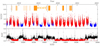 |
Fig. 1. Long-term behavior of Cygnus X-1 measured by all-sky monitors MAXI and Swift-BAT. We follow the same approaches of state definition proposed by Grinberg et al. (2013). Upper panel: the hard, intermediate, and soft states are denoted by blue, purple, and red points, respectively. Lower panel: the unclassified and soft states are plotted with black and red points, respectively. The duration of HXMT observations on Cygnus X-1 is shown in dark orange stripes at the top. |
Start dates and end dates of the HXMT observations.
2.1. Data extraction
We use the pipeline based on Insight–HXMT Data Analysis Software (HXMTDAS) v2.04 along with the latest calibration database v2.05 to process the observational data. The good time intervals (GTIs) are selected according to the following criteria: an elevation angle (ELV) larger than 10°, a geometric cut-off rigidity (COR) larger than 8 GeV, an offset angle from the pointing direction (ANG_DIST) smaller than 0.04°, and at least 300 s before and after the South Atlantic Anomaly (SAA) passage. For the LE telescope, we adopt an additional criterion that the elevation angle for the bright Earth is larger than 30°. The individual detectors of the HXMT instruments have different fields of view (FoVs). Given that Cygnus X-1 is a bright source, we use photon events generated by the detectors with a small FoV for the following analysis.
In our analysis, we consider those GTIs that are covered by all three instruments and that are longer than the individual segment used for timing analysis, that is, longer than 16 s. In our timing analyses, we therefore used a total 145 exposures, for which we have obtained energy spectra. We use ISIS 1.6.2 (Houck & Denicola 2000) – which allows access to the defined models in Xspec (Arnaud 1996) – to perform the spectral fitting. The energy bands for the spectral analyses are 2−10 keV for LE, 10−30 keV for ME, and 28−120 keV for HE. We use the tools LEBKGMAP, MEBKGMAP, and HEBKGMAP provided by the HXMT team to estimate the instrumental background (Liao et al. 2020a,b; Guo et al. 2020).
The light curves for timing analyses are generated by the corresponding event lists from the detectors with a small FoV directly, processed with Stingray (Bachetti et al. 2021; Huppenkothen et al. 2019a,b). The selected energy range is 1−10 keV for LE, 10−30 keV for ME, and 30−150 keV for HE. In order to study the energy-dependent properties, the energy range of LE was divided into four bands: 1−3 keV, 3−5 keV, 5−7 keV, and 7−10 keV; ME was divided into two bands: 10−20 keV and 20−30 keV; HE was divided into three bands: 30−50 keV, 50−90 keV, and 90v150 keV. In the following, whenever hardnesses are discussed, they are calculated using raw photon counts, not fluxes. The time resolution of those light curves is set to 2−9 s ≈2 ms. As we are using the fast Fourier transform for our calculations, we use segments with a length of 213 × Δt = 16 s to calculate timing properties. The dead time of the LE telescope is negligible, and set to zero (Chen et al. 2020); the dead time of ME and HE are set to 200 μs and 2 μs, respectively (Cao et al. 2020; Liu et al. 2020). The power spectral densities (PSDs) are Poisson-noise and dead-time corrected according to Zhang et al. (1995). Thus, the Nyquist frequency for the light curves is fmax = 1/(2Δt) = 256 Hz, and the lowest frequency we can access is fmin = 1/(nbinsΔt) = 0.0625 Hz.
2.2. Long-term source behavior
Different from the majority of the transient BHBs that trace the canonical q-track during the outburst, Cygnus X-1 is one of the only few known persistent BHBs, and is fed by the wind from its companion. It has been bright since its discovery, and often moves between the hard state and the soft state, without tracing any q-track (e.g., Wilms et al. 2006; Fender et al. 2006; Grinberg et al. 2013). Previous studies showed that Cygnus X-1 spends most of the time in the hard state and the soft state, which indicates that these two states are more stable than the intermediate state (see e.g., Grinberg et al. 2013; Meyer-Hofmeister et al. 2020). Prior to ∼2011, the source has spent most of the time in the hard state, with only occasional excursions toward the soft (Grinberg et al. 2013, 2014). Since then and within the life time of MAXI, it has mainly been in the soft state (Cangemi et al. 2021); the reason for this is not yet known.
Pottschmidt et al. (2003) report “failed transitions” frequently observed in Cygnus X-1: the source softens, but never reaches a proper soft state, instead eventually returning to the hard state. Similar failed transitions have also been observed in transient BHBs (e.g., GX 339−4, see Fürst et al. 2015; García et al. 2019; and Swift J1753.5−0127, see Bu et al. 2019). Although enormous amounts of data have been collected over decades, the true mechanism of state transitions and the reason why BHBs maintain their stability particularly in the hard and soft states are still open questions.
Here we use the LE data of the three proposals in Table 1 to produce the HID for Cygnus X-1, as shown in Fig. 2. The data from proposals P0101315 and P0305079 cover the soft state and the intermediate state. However, the proposal P0201012 contains observations in the hard state, enabling us to compare source properties across all states.
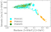 |
Fig. 2. HID of Cygnus X-1 using the data from three proposals: P0101315, P0201012, and P0305079, that are denoted by cyan, orange, and green, respectively. The intensity is defined by the photon count rate of LE ranging from 1 to 10 keV. We define the hardness as the ratio of the raw photon count rate between the 5−10 keV band and the 1−5 keV band. The time resolution is set to 60 s. |
3. Spectral analysis
3.1. Spectral modeling
For a spectral-timing study of numerous observation samples presented here, a reliable but simple characterization of the spectral shape is necessary. Former long-term spectral studies of Cygnus X-1 used a simple phenomenological model consisting of a broken power law modified by a high-energy cut-off and a disk component to fit the energy spectra (Wilms et al. 2006; Böck et al. 2011; Grinberg et al. 2014). We can write the model as:

where tbabs calculates the photons absorbed by the interstellar medium, whose cross-sections are provided by Verner et al. (1996) and the element abundances are given by Wilms et al. (2000).
Bknpower × highecut empirically describes a continuum that dominates the spectrum in the hard X-ray band. Bknpower has three parameters except its normalization: Γ1, the photon index of the soft band; Γ2, the index of the hard band, and the breaking energy Ebreak, in our case around 10 keV. We also included a Gaussian line in the fit in order to characterize the iron Kα line emission located at around 6.4 keV. Finally, we used diskbb, a multi-temperature disk model, to fit the thermal radiation from the accretion disk (Mitsuda et al. 1984; Makishima et al. 1986). Typical spectra for Cygnus X-1 are shown in Fig. 3. In the hard state, the disk component never dominates the spectrum. However, the thermal component plays a significant role at soft X-rays when the source is in the soft state.
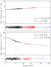 |
Fig. 3. Typical spectra of Cygnus X-1 with HXMT observations. Upper panel: a spectrum in the hard state (obs ID: P0201012171). The spectrum in the lower panel: is in the soft state (obs ID: P0101315057). Data from the LE, ME, and HE telescopes are denoted with black, red, and blue crosses, respectively. The power-law continuum, the thermal component, and the iron line emission are indicated with dashed lines. |
For our study, this simple phenomenological modelization is sufficient to identify the different spectral component, but we note here that using a more sophisticated physical model to fit the spectra, involving more parameters and more complex assumptions, would be a worthwhile alternative (for a recent study using a physical model on Cygnus X-1 with the HXMT data, see e.g., Feng et al. 2022).
The data coming from all instruments are rebinned to a minimum signal-to-noise ratio of 10. Considering the accuracy of the current calibration and that Cygnus X-1 is a bright source, we adopt a systematic error of 0.5%, 0.5%, and 1.0% for LE, ME, and HE, respectively (Li et al. 2020; Kong et al. 2021). The peak energy of gaussian is fixed at 6.4 keV, and the column density NH is fixed at the value of 7.1 × 1021 cm−2, as given by the measurements of the HI4PI survey based on EBHIS and GASS (HI4PI Collaboration 2016). All the other parameters remain free.
While in general we expect NH to be variable in Cygnus X-1, especially during the hard state (e.g., Grinberg et al. 2015; Hirsch et al. 2019; Lai et al. 2022), only a handful of our observations are in the hard state at the orbital phases where they could be affected. In the soft state, the state in which Cygnus X-1 is found in most of our observations, the wind is expected to be highly ionized and thus would contribute little to the observed absorption. The NH measurements obtained from our HXMT data if the absorption column density is left free to vary show trends that we interpret as systematic effects. In particular, in Fig. 4 (in black), we can see a clear increase in NH for higher Γ1, which we interpret as due to the strong contribution of the steep power law at low energy and the degeneracies between the power law, disk, and absorption contributions. This is particularly the case when the power law is steep and the contribution of the disk is strong, because the simple power-law model, which does not have a low-energy cut-off, extends below the energies of the putative seed photon contribution (i.e., the diskbb component) for the Comptonization component it is describing. Similar overestimation of NH can also be seen in Böck et al. (2011) and Grinberg et al. (2015), for example, where the high NH are associated with high uncertainties. We conduct an additional test by extending the lower limit of our spectra to 1.5 keV, taking advantage of the LE instrument response. We obtain better constraints on NH, which are very close to the value suggested by the HI4PI survey (Fig. 4, in red). As this work does not focus on the contribution of the stellar wind but aims to obtain a satisfactory continuum description, we interpret this as confirming our choice to fix the NH value, but caution that detailed disk and wind studies would require a careful consideration of possible calibration effects and model degeneracies.
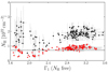 |
Fig. 4. Soft photon index Γ1 of bknpower obtained by free column densities versus the obtained column densities NH during the absorption. The black dots indicate the NH obtained by the spectral fitting down to 2 keV; while the red dots indicate the NH obtained down to 1.5 keV. The dashed line represents the value 7.1 × 1021 cm−2, which is adopted during our spectral fitting. |
Overall, we are able to obtain good fits for all our spectra as shown in Fig. 5, where we also show the quality of fits obtained when the column density is left free.
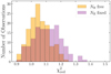 |
Fig. 5. Histogram of the reduced χ2 over the best fits of the 145 spectra. Most of the |


3.2. Discussion of spectral modeling
We first verify the validity of our spectral modeling by checking the correlations between the spectral hardness and soft photon index Γ1, and between the ratio of unabsorbed energy flux directly from the thermal radiation (diskbb-model) over the total unabsorbed energy flux in the 2−5 keV range and Γ1, as shown in the first two panels in Fig. 6. Both show the correlations expected for hard to soft transition.
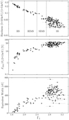 |
Fig. 6. Spectral evolution versus the soft photon index Γ1. Top panel: correlations of the 5−10 keV/1−5 keV hardness versus Γ1. We define the hard state (HS), the hard intermediate state (HIMS), the soft intermediate state (SIMS), and the soft state (SS) with Γ1 values. Middle panel: ratio of unabsorbed energy flux of the disk components over the total energy flux versus Γ1. Bottom panel: intensity of reflection that is denoted by the equivalent widths of the iron Kα lines, and is stronger in the soft state than in the harder state. |
We can now define the state of the source by the corresponding value of Γ1: the hard state for Γ1 ≤ 2.0, the hard intermediate state for 2.0 < Γ1 ≤ 2.4, the soft intermediate state for 2.4 < Γ1 ≤ 2.7, and the soft state if Γ1 > 2.7. Our choice is supported by the sudden change of the PSD shape in the 3−5 keV band and the intrinsic coherence in the 1−3 versus 3−5 keV band; see Sects. 5.2 and 5.3 for more details, as well as Grinberg et al. (2014).
The positive correlation between the intensity of the reflection – shown by the equivalent width of the iron Kα line – and the spectral parameter Γ1 is presented in the bottom panel of Fig. 6. This result is consistent with the findings of Gilfanov et al. (1999), Ibragimov et al. (2005), Shaposhnikov & Titarchuk (2006), and Steiner et al. (2016) for example, all of whom used RXTE data for their analyses.
By studying Cygnus X-1, Shaposhnikov & Titarchuk (2006) propose that the corona may have a compact geometry in the intermediate and soft states. Based on observations of 29 stellar-mass BH candidates, Steiner et al. (2016) offer two interpretations. One agrees with Shaposhnikov & Titarchuk (2006) that the size of the corona shrinks when the state softens, and the other agrees with Petrucci et al. (2001), who discuss the Comptonization effect on the reflection component, stating that in the hard state, the iron line amplitude will be diluted by Compton scattering due to the higher optical depth of the corona.
The intensity of the reflection can be roughly quantified by the difference between the two photon indices as well, as the model combination bknpower × highecut with the breaking energy around 10 keV is capable of characterizing the Compton hump around 20−30 keV (Wilms et al. 2006). We present the correlations of two photon indices and the difference between them, ΔΓ, in Fig. 7, and ΔΓ versus the equivalent widths of the iron lines in Fig. 8. Consistent with the apparent relationship between the equivalent width and Γ1, we see a clear positive trend between ΔΓ and Γ1. In addition, Fig. 8 shows that the two indicators of the reflectional strength are indeed positively correlated even in the soft state. We therefore conclude that in the soft state, the reflection is indeed stronger than in the hard state.
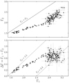 |
Fig. 7. Upper panel: soft photon index Γ1 versus the hard photon index Γ2 in model bknpower. The dashed line indicates that Γ1 = Γ2. Lower panel: the correlations between Γ1 and the difference of two photon indices, defined by ΔΓ = Γ1 − Γ2, are shown. The lines that are parallel to the dotted lines indicate a constant Γ2. |
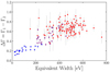 |
Fig. 8. The correlation of ΔΓ versus the equivalent widths of the iron Kα lines. The blue/purple/red points denote that the source is in the hard/intermediate/soft state, respectively. |
However, the correlation we observe between Γ1 and Γ2 shows a “bend” at Γ1 ≈ 2.7 as shown in the upper panel of Fig. 7. This is coincident with the onset of the soft state and fits where the uncertainties on the current steep power-law index are larger. Similar trends were not observed by Wilms et al. (2006), who did not include a disk for their fits in the soft state, resulting in a poor description of the spectra below 6 keV. We check whether our choice to freeze NH may lead to the observed bend in the correlation: We find that for Γ1 (NH fixed)≳2.7, an evident deviation between the Γ1s with fixed and free NH appears (see Fig. 9). Still, the bend in the correlation appears even for free NH, meaning that it is not purely an artifact of the choice of parameter space for our model.
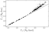 |
Fig. 9. The soft photon index Γ1 of bknpower obtained by fixed NH = 7.1 × 1021 cm−2 and free NH. The dashed line indicates that Γ1 (NH fixed) = Γ1 (NH fixed). |
4. Energy-resolved variability properties
4.1. Power spectra and the fractional rms
Power spectra (also power spectral densities, or PSDs), are the first-order products of the discrete Fourier transform performed on a time series, and their calculations are discussed in detail by Nowak et al. (1999), for example; see their Sect. 2. The power spectra are calculated in units of rms fluctuations scaled to the mean count rate (Belloni & Hasinger 1990a; Miyamoto et al. 1991). This normalization is often employed, as it is convenient to compare the power spectra from different states or even different sources, because the variance that each frequency contributes is independent of the averaged photon count rate. The total fractional rms is the integral of the PSDs over all available frequencies, which in our case is 0.0625 − 256 Hz.
In some of the energy bands considered for our analysis, the background photons contribute significantly. Especially in the soft state, they dominate in the hard X-ray bands and need to be taken into account. We therefore adopt a background correction for the fractional rms (Belloni & Hasinger 1990b; Bu et al. 2015):
 (1)
(1)
where P is the noise-subtracted power normalized according to Miyamoto et al. (1991), and S and B are the averaged photon count rates from the source and the background, respectively. This background correction adds a factor (S + B)/S – the value of which is always greater than 1 – to the raw rms values. This implies the assumption that the background is intrinsically invariant and therefore does not contribute to the total variability. As expected, this assumption is not true when background noise dominates the data, and will lead to the overestimation of the fractional rms, because the background noise has its own intrinsic variability as well.
Figure 10 shows the correlations of different estimates of total rms with spectral shape as represented by Γ1 for all instruments and energy ranges under consideration. To present the effect of the employed background correction, we additionally show the inverse of the correction factor, [(S + B)/S]−1 = S/(S + B). For S/(S + B) close to 1, most of the photons come from the source, and therefore the corrected rms is almost equal to the raw rms. The corrected rms is higher than the raw rms when S/(S + B) < 1. As some of the data with a high Γ1 are very noisy, we use smooth curves calculated through simple interpolation between data points to present the macroscopic trends between the total rms and Γ1.
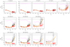 |
Fig. 10. Correlations between the soft photon index Γ1 and the fractional rms from all the instruments on HXMT. The red circles are the raw rms without the correction of Eq. (1), and the black dots are the corrected total rms according to Eq. (1). The magenta dotted lines denote the signal-to-background ratio S/(S + B). The orange solid lines show the trends of the corrected and uncorrected total rms when varying Γ1. |
4.2. Evolution of the power spectral density with spectral shape
We follow the approach of Böck et al. (2011) and Grinberg et al. (2014) to visualize the whole power spectra by color maps in Γ1-fi-space. The values of Γ1 are obtained from the best fits from Sect. 3, where Γ1, min = 1.63 and Γ1, max = 3.27. The grid of Γ1 is defined linearly by constant steps of ΔΓ1 = 0.1 between the two limits. The power spectra from different observations will be averaged if their Γ1 belongs to the same bin of the grid. The frequencies f are rebinned logarithmically between 0.0625 Hz and 256 Hz, with an equally spaced grid in logarithmic scale df/f = 0.15. The evolution of the PSD shape versus Γ1 is shown in Fig. 11.
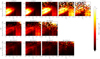 |
Fig. 11. Evolution of PSDs versus the soft photon index Γ1 from different energy bands provided by all instruments on HXMT. The color scale represents the average value of PSD(fi)×fi at individual frequencies fi. Please note that the PSD values in these plots have not been corrected by Eq. (1) in order to avoid the covering effect due to the high signal-to-background ratio. |
The PSDs shown in Fig. 11 have not been corrected by Eq. (1), and therefore the integral over all frequencies corresponds to the uncorrected rms shown in Fig. 10. We can also see that the strength of the variability from HE bands is weaker than that from ME bands. The main reason is that the background photons that significantly contribute to the harder X-ray bands will elevate the detected count rate, which leads to underestimation of the strength of the intrinsic variability of the source. To clearly show the evolution of the variability above 30 keV, we rescale the color map of HE bands; see Fig. 12.
 |
Fig. 12. Same as the last row of Fig. 11, but with a different color scale in order to illustrate the evolution of the variability component more clearly. |
Figures A.1–A.3 show the averaged PSD shapes versus Γ1 for all the three instruments. We note that ME and HE bands are both dominated by background photons when Cygnus X-1 is in the extreme soft state. The flux in those bands is weak, and the uncertainties of the Fourier signals at high frequency bands are large. In this case, those PSDs should not be considered as physical.
4.3. Coherence function and phase-lags
The coherence, as well as the phase-lags, are the products of Fourier transform between two simultaneous light-curve series. Usually we study these quantities between two different energy bands, to identify the lost phase-related information when we compute the moduli of the products of Fourier transform. The intrinsic coherence function, γ2(f), is defined by Vaughan & Nowak (1997), where the auxiliary quantity n2 defined in Eq. (4) by Vaughan & Nowak (1997) is the expectation of the noise contribution.
The coherence function itself is a frequency-dependent measurement of the linear correlation between two simultaneous time series. In principle, the coherence function ranges from 0 to 1, where 0 means no coherence and 1 means perfect linear coherence. But when considering the noise correction, we possibly obtain a coherence of greater than 1 or even negative. A negative coherence can merely emerge if the noise dominates one of the power spectra. In this case, the negative coherence there does not make sense. However, a coherence of greater than 1 may be seen even when the signals at that frequency are well measured. This is due to the fact that the auxiliary quantity n2 cannot be estimated well when there are insufficient segments, or when the signals from two bands correlate extraordinarily strongly. Therefore, a coherence of higher than 1 still means good linear correlation between the two light curves and is not considered problematic in the following parts of the analysis.
We follow the same recipe to present the coherence function in Γ1-fi-space, as shown on the left-hand side of Fig. 13. Similarly to Figs. 11 and 12, we use a thermal color map to visualize the coherence, where brighter colors represent better coherence, and dimmer colors represent poorer coherence. We can see a clear envelope located at ∼10 Hz in each panel on the left-hand side of Fig. 13, and above ∼10 Hz, the noise-subtracted power densities are close to zero and the coherence fluctuates violently.
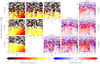 |
Fig. 13. Evolution of the coherence function γ2 and the phase-lags versus the soft photon index Γ1 between different energy bands of the LE telescope. |
The three panels in the first column of Fig. 13 are the coherence functions of the softest band (1−3 keV) versus the other harder bands (3−5 keV, 5−7 keV, and 7−10 keV). In the hard state and the hard intermediate state, where 1.6 ≤ Γ1 ≲ 2.4, the coherence function in the 1−3 keV versus 3−5 keV band is quite close to 1. But in the soft intermediate state and the soft state, where 2.4 ≲ Γ1 ≲ 3.3, the loss of coherence emerges at low frequencies. A similar loss of coherence can also be found in the 1−3 keV versus 5−7 keV band and the 1−3 keV versus 7−10 keV band. The loss of coherence in the soft/intermediate state in these bands is due to the fact that the dominant spectral component in the 1−3 keV band has changed during the state transition. In the hard state, where Γ1 ≤ 2.0, the 1−3 keV band is dominated by the power-law emission. But in the soft state, where Γ1 ≳ 2.7, the thermal emission from the disk becomes dominant. As expected, and as the dominant emission comes from spatially distinct regions, we observe a loss of coherence.
When the two energy bands are both power-law dominated, the loss of coherence in the soft state disappears, which can be seen in the remaining three panels on the left-hand side of Fig. 13. We obtain the best coherence for nearly all Γ1 values in 3−5 keV versus 5−7 keV band.
On the right-hand side of Fig. 13, we show the frequency-dependent phase-lags between different energy bands of LE, but using a different color map. Hard lags are denoted in red, while soft lags are denoted in blue. For ME and HE data, the coherence and the phase-lags are noisier and cannot be visualized using this approach. Instead, we show the averaged coherence function and the averaged phase-lags taken over the frequency band and Γ1 band. Inspired by the coherence evolution in 1−3 keV versus 3−5 keV band, we divide the soft photon index Γ1 into five sub-bands: 1.6−2.0, 2.0−2.4, 2.4−2.7, 2.7−3.0, and 3.0−3.3, consistent with the state definitions in Sect. 3.2. We first rebin the raw coherence and phase-lag spectra to a logarithmically spaced frequency grid with df/f = 0.15, and average the coherence and the phase-lag in the 0.0625−6 Hz frequency range in each Γ1 band. Here, we correct any coherence greater than 1 (mostly seen in the HE data) to simply 1 in order to cancel the effect of strong correlation when averaging. The results are shown in Figs. 14 and 15.
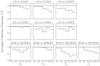 |
Fig. 14. Evolution of the coherence ⟨γ2⟩ averaged over the 0.0625−6 Hz frequency range versus the states (classified by the soft photon index Γ1) between different energy bands. |
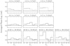 |
Fig. 15. Similar to Fig. 14, but with the evolution of the average phase-lag versus the states (classified by the soft photon index Γ1). In the first three panels, the average phase-lags with Γ1 ≥ 2.4 are denoted by dotted lines, as we know that the loss of coherence is due to the different emission origins. |
5. Discussion of the timing properties
5.1. The total fractional rms
We show both corrected and uncorrected rms in Fig. 10 in order to underline the differences between them. For LE, the signal-to-background ratio is higher than 75%, and the differences between the two rms estimates can be ignored, as clearly seen in the upper row of Fig. 10. However, when a non-negligible fraction of photons comes from the background, they inevitably smear the power spectrum and the rms. In order to obtain the true trends of total rms using the available data, our assumption can be stated as follows: (1) The raw rms is true if the background has the same intrinsic variability as the source; (2) the corrected rms is true if the background rate is intrinsically invariant and does not contribute to the total variability at all; and (3) the true value should lie between the two extreme cases above: the background has its own intrinsic variability, but in all cases, the variability from the source dominates. Therefore, the true total rms should be between the two trends (denoted by the two orange solid lines) in all panels in Fig. 10. Along with the improved quality of the data, the two curves that represent the two extreme cases become closer, and the uncertainty range of the true trend is smaller.
As shown in Fig. 10, the macroscopic positive trends between the total rms and Γ1 in hard X-ray bands in the soft state challenge the well-known statement that, due to the domination of the thermal emission in the soft state, the total rms is much lower than that in the hard state (e.g., Belloni et al. 2005; Heil et al. 2015). We note that this statement is only true when the soft X-ray band – that is dominated by thermal photons in the soft state – is contained (e.g., 1−3 keV band or 1−10 keV band). The exact reason for this is discussed in Sect. 5.2. For other, harder bands, where Comptonized photons dominate even in the soft state, indeed we see a slightly negative trend when Γ1 ≲ 2.7, and a positive trend when Γ1 ≳ 2.7.
The total rms works as an integral of the PSDs over all available frequencies. Different fractional rms values doubtlessly tell us that the properties of the source radiation are different, but even with a flat correlation of rms-Γ1, such as that shown in the 5.0−7.0 keV band in Fig. 10, the timing properties in soft and hard states are still quite different. These properties can be revealed by the PSD evolution with spectral shape, which is presented and discussed in Sects. 4.2 and 5.2.
5.2. Evolution of the PSD
Our work extends the previous RXTE-based analysis, which covered the 2.1−15 keV range (Böck et al. 2011; Grinberg et al. 2014), to both lower and higher energies. Our maps therefore allow us to better trace both the variability of the disk that contributes to the lowest energies and the variability of the high-energy part of the power law.
In Fig. 11, we see a clear boundary at Γ1 ≃ 2.7. Before this boundary, there are at least two pronounced variability components in the 1−10 Hz range. Their frequency increases when the source softens.
The central frequencies are approximately independent of the energy bands (for similar results recently obtained for other BHBs, see e.g., Ma et al. 2021). The power spectra of Cygnus X-1 in the hard and intermediate states are comparatively smooth and without narrow features (see e.g., Axelsson et al. 2005, 2006; Rapisarda et al. 2017). While we acknowledge that there is some confusion in the literature, with the broad variability components having been referred to as quasi-periodic oscillations (QPOs) in past analyses (Gilfanov et al. 1999; Shaposhnikov & Titarchuk 2006), the behavior of the observed variability components does not agree with the established definition of LFQPOs (see e.g., Ingram & Motta 2019).
Following Grinberg et al. (2014), we label the variability component with a lower central frequency as “Component 1” and that with a higher central frequency as “Component 2”. We can see a gradual growth of the strength of Component 2, but Component 1 fades when the X-ray bands become harder. The Component 2 becomes dominant above ∼10 keV. Here, we can, for the first time, trace this behavior above ∼15 keV.
We are able to trace the variability components, especially Component 2, in the hard state and their increasing frequency with an increasing Γ1 to at least the 50−90 keV range. This is especially clearly visible in Fig. 12 where we rescale the map colors to account for the overall low variability detected in the HE instrument.
The maps in the 90−150 keV range do not show a clear pattern. This band is especially interesting since the spectral cutoff in the hard intermediate state is around ∼150 keV (Wilms et al. 2006, and our fits in this analysis), with a polarized hard tail present above these energies (Laurent et al. 2011; Jourdain et al. 2012; Rodriguez et al. 2015; Cangemi et al. 2021). To enhance the signal, we calculate the average PSDs for four states defined by Γ1 values, the hard state (Γ1 ≤ 2.0), the hard intermediate state (2.0 < Γ1 ≤ 2.4), the soft intermediate state (2.4 < Γ1 ≤ 2.7), and the soft state (Γ1 > 2.7) (see Fig. 16). However, the power spectra in the 90−150 keV band are still too noisy to allow firm conclusions to be drawn. Nevertheless, we do see an overall decrease in variability, in agreement with previous results using INTEGRAL/SPI (Cabanac et al. 2011).
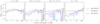 |
Fig. 16. Average power spectra calculated from light curves obtained from the HE instrument in different energy bands in four different Γ1 ranges. The PSDs for the 30−50 keV band, 50−90 keV band, and 90−150 keV band are denoted with black, red, and blue lines, respectively. The PSDs are rebinned to df/f = 0.3. |
In the prior studies of Cygnus X-1, the variability components seen in the hard and intermediate states can be well modeled by usually two Lorentzians with different central frequencies (Nowak 2000). Consistent with for example Cui et al. (1997a), Gilfanov et al. (1999), Pottschmidt et al. (2003), Axelsson et al. (2006), Shaposhnikov & Titarchuk (2006), and Böck et al. (2011), who studied the evolution of the behavior of these components, we find that their central frequencies increase as the source softens. The strength of components in the 1−10 Hz band directly determines the total fractional rms that is shown in Fig. 10. For those bands above 3 keV, the total rms slightly drops during the hard-to-intermediate transition, where 1.6 ≲ Γ1 ≲ 2.7. But the variability in the 1−3 keV band is additionally influenced by the thermal photons from the accretion disk. The thermal photons that present red-noise spectra in the PSDs make the variability of the smooth components fade more quickly than the harder bands. This is the exact reason why we see a continuously decreasing value of the total rms only in the 1−3 keV band or the 1−10 keV band during the softening of the state.
When the source continues its transition to the soft state, crossing the boundary of Γ1 ≃ 2.7, the power spectrum of hard X-ray bands suddenly changes to a red-noise spectrum with a slope of f−1 below 10 Hz. A similar behavior of the PSD evolution was also reported by Grinberg et al. (2014) at energies up to 15 keV and is traced here for the first time at higher energies, where the power law is the dominating spectral component even in the soft state. The sudden change of the PSD shape at Γ1 ≃ 2.7 is the reason why the total rms has a positive tail versus Γ1 in the hard X-ray bands.
In the soft state of Cygnus X-1, with Γ1 ≳ 2.7, the PSD shape shows a red-noise spectrum with a slope of f−1 below 10 Hz (see e.g., Cui et al. 1997a,b; Gilfanov et al. 2000; Churazov et al. 2001; Pottschmidt et al. 2003; Axelsson et al. 2005; Grinberg et al. 2014). Cui et al. (1997a) and Churazov et al. (2001) also state that the red-noise variability becomes stronger when our focused energy range moves to the harder X-ray bands. This is confirmed by the higher total rms shown by the positive tails of the trends of the corrected rms in Fig. 10 and the brightness of the PSD shapes in Fig. 11.
5.3. The coherence function and the phase-lags
Figure 14 shows that, in the soft state where Γ1 ≥ 2.7, the HE data (≥30 keV) and the LE data involving the 1−3 keV band tend to have poorer coherence than those with lower Γ1s. The loss of coherence in LE data is interpreted by the domination of the thermal photons from the disk in the 1−3 keV band. But the loss in HE data is mainly due to the low signal-to-background ratio when Γ1 ≥ 2.7. Here we note that Grinberg et al. (2014) do not find similar loss of coherence due to the thermal photons with RXTE/PCA data, as the lower limit of their softest energy band is 2.1 keV, which in our case is 1.0 keV. In order to check this supposition, we also extract the event lists from LE for photons of 2.1−4.5 keV and compute the coherence involving this new energy band. We do not see evident loss of coherence in the soft state. This fact indicates that the thermal photons may dominate the 1−3 keV band, but cannot dominate the 2.1−4.5 keV band in the soft state of Cygnus X-1.
In addition, in those bands where the coherence can be well measured, we can see a coherence decrease where 2.4 ≲ Γ1 ≲ 2.7. Grinberg et al. (2014) report a similar loss of coherence when 2.35 ≲ Γ1 ≲ 2.65 based on an analysis of the RXTE/PCA data for Cygnus X-1. The origin of the loss of coherence in this soft intermediate state has not been ascertained. Considering that the jet emission in this state becomes weak and unstable or even hardly detectable (e.g., Fender et al. 2004; Böck et al. 2011; Corbel et al. 2013), the loss of coherence is highly possibly connected with the unstable jet base.
As the different origins of the emission in the 1−3 keV band in the hard and the soft state are confirmed by previous spectral and timing analyses, we denote those phase-lags where Γ1 ≥ 2.4 with dotted lines in Fig. 15, and do not discuss them further, because there the quality of the linear coherence between two light curves is poor.
Figure 13 shows that the dominant hard lags contribute from the 1−10 Hz band when Cygnus X-1 is in the intermediate state. In the hard state, hard lags tend to be generated at slightly lower frequencies, in comparison with those in the intermediate state. This consistency of the central frequencies of the variability components and the dominant contribution of the frequency-dependent phase-lags indicates that the lags of the hard photons are likely related to the variability components. However, the phase-lags in the soft state in general stochastically fluctuate around zero, resulting in a sudden drop in the average phase-lags when Γ1 > 2.7, which is shown in Fig. 15.
Most of the average phase-lags in Fig. 15 are positive, which means that in our data, the hard photons usually lag the soft photons. Similar hard lags observed on Cygnus X-1 are also reported; for example, by Cui et al. (1997a), Nowak et al. (1999), Pottschmidt et al. (2003), Böck et al. (2011), and Grinberg et al. (2014).
We are particularly interested in the average phase-lags between the adjacent energy bands (e.g., 3−5 keV vs. 5−7 keV band or 10−20 keV vs. 20−30 keV band), because the phase-lags between the nonadjacent bands can be estimated by summing the phase-lags between the adjacent bands in one 2π period if the coherence remains good. From the 3−5 keV vs. 5−7 keV band, the 5−7 keV vs. 7−10 keV band, and the 10−20 keV vs. 20−30 keV band in Fig. 15, we see that the average phase-lags in the 0.0625−6 Hz band always increase as the state softens, where Γ1 transitions from 1.6 to 2.7. But when Γ1 continues to increase, the average phase-lags will decrease. In our work, the maximum lags are observed in the soft intermediate state, where 2.4 ≲ Γ1 ≲ 2.7. Grinberg et al. (2014) reported the lag evolution with RXTE/PCA data on Cygnus X-1, with their maximum values consistently at Γ ≃ 2.65, but using the form of time-lags, suggesting that the geometry of the corona shows a sudden change, which was indicated by the sudden change of the PSD shape as well.
Intriguingly, this positive correlation between the average phase-lags and Γ1 no longer holds in the 1−3 keV vs. 3−5 keV band, when the source transitions from the hard to hard intermediate state, where 1.6 ≲ Γ1 ≲ 2.4, as shown in Figs. 13 and 15. Figure 13 indicates that the dominant hard lags are contributed from the hard and hard intermediate states, within the frequency band of the variability components. In Fig. 15 we can see that the phase-lags decrease slightly as Γ1 increases. The coherence there is good and the measured phase-lags are accurate. This phenomenon may suggest that in the hard state, although both the 1−3 keV band and the 3−5 keV band are both dominated by power-law photons, the 1−3 keV band is more likely to be dominated by the seed photons, which are possibly produced by the thermal black-body radiation of the accretion disk or the synchrotron radiation in the jet base; while the 3−5 keV band is dominated by the Comptonized photons up-scattered from the seed photons in softer X-ray bands.
6. Variability properties of Cygnus X-1 in a larger context
So far, we have discussed the individual variability properties of Cygnus X-1 (Sects. 5.1–5.3). We now discuss our results in the context of mechanisms of state transition, the disk-corona model, and the plausible scenarios of accretion in BHB systems.
6.1. Comparison with the behaviors of other BHBs
Cygnus X-1 is a persistently luminous BHB fed by the wind of its companion. However, the majority of BHBs are transient. Although we expect similar accretion scenarios for both kinds of system, it is still meaningful to compare the phenomenology observed for Cygnus X-1 with other known BHBs.
The total fractional rms, which is the integral of PSDs over all frequencies, decreases as the state softens (Belloni et al. 2005). This is also observed in transient and other persistent BHBs (e.g., Remillard & McClintock 2006). However, as discussed in Sect. 5.1, we should always outline the chosen energy band when defining the total rms, as different energy bands give different trends.
The evolution of the power spectra during state transitions has been reported in other BHBs, such as GX 339−4 (Zdziarski et al. 2004; Motta et al. 2011; Shui et al. 2021), GRS 1915+105 (Soleri et al. 2008; Ueda et al. 2009), XTE J1550−564 (Sobczak et al. 2000; Rodriguez et al. 2004; Rao et al. 2010), 4U 1630−47 (Tomsick & Kaaret 2000), and Swift J1753.5−0127 (Soleri et al. 2013; Bu et al. 2019). Most of the transient BHBs show narrow features in their power spectra, classified into type A, B, and C LFQPOs by their central frequencies, time-lags, and the quality factor (Casella et al. 2005; Motta et al. 2015). The central frequencies of the LFQPO components rise when the state of the BHB softens, and drop when returning back to the hard state (Vignarca et al. 2003). Sobczak et al. (2000) also reported an exception, GRO J1655−40, which shows a negative correlation of the central frequency of the 14−28 Hz LFQPO versus the power-law index, but a positive correlation with the disk flux, during a transition from very high state to the usual soft state. However, Motta et al. (2012) confirmed that the central frequencies of the LFQPO components still increase during the hard-to-soft transition. We note here that the transition from the very high state to the soft may not follow the regulation we talk about, and GRO J1655−40 is also special, as the HFQPO component and more than two LFQPO components can be observed (Strohmayer 2001; Belloni et al. 2012).
When those sources complete their transition from the hard state to the soft state, their power spectra with narrow or smooth peaks will be substituted by a red-noise power spectra with f−1 slope (see e.g., Miyamoto et al. 1994; Remillard & McClintock 2006; Ueda et al. 2009; Klein-Wolt & van der Klis 2008; Mao & Yu 2021), although Cygnus X-1 generally shows a higher overall variability than transients in the the soft state (e.g., Heil et al. 2015).
Fewer studies have addressed the higher order timing properties (the coherence function and phase/time-lag). Reig et al. (2018) report the growth of the hard lag of eight BHBs when the sources undergo a hard-to-intermediate transition. Altamirano & Méndez (2015) additionally find a sudden decrease in the averaged phase-lag at the transition point between the intermediate state and the soft state in GX 339−4, which is consistent with Grinberg et al. (2014) and our results.
6.2. Current models to describe timing properties
All the timing studies presented and discussed in Sects. 4 and 5 conclude that the variability components are strongly correlated with the mechanism of the transition between the hard and the soft state. Therefore, interpretation of their origin is crucial in order to reveal the accretion scenario.
Böck et al. (2011) reported a fast state transition in Cygnus X-1 within less than 2.5 h, but with their available data, they could only reach the soft intermediate state with Γ1 < 2.7. The sudden change in the PSD from distinct variability components to red-noise spectrum has not been observed.
The variability components seen in the PSDs of Cygnus X-1 are smooth, with a quality factor Q ≲ 1 modeled by two Lorentzian curves (e.g., Böck et al. 2011). Therefore, the models developed for the LFQPOs – for example, the Lense-Thirring precession (Bardeen & Petterson 1975) or the accretion-ejection instability (Tagger & Pellat 1999) – are not suitable in our case. Besides, even for the narrow LFQPOs commonly seen in other transient BHBs, we do not yet have a satisfying physical model that can consistently explain the spectral and timing behaviors (see Ingram & Motta 2019 for a recent review).
Among those models, a large fraction of them assume a truncated disk and hot inner flow geometry. In this scenario, the hard-to-soft transition happens when the truncation radius between the standard disk and the hot accretion flow decreases, which means an increasing characteristic frequency for all variabilities. Fruitful developments have been made by applying this scenario. For instance, Ingram et al. (2009) consider the precession of a hot flow inside a truncated disk, which is able to explain why the observed maximum frequency is almost constant for all BHBs. Ingram & Done (2011) further include the effect of the local fluctuations in the mass accretion rate in the model, which can reproduce the PSD shapes that are commonly seen in real data. Recently, Kawamura et al. (2022) considered propagating mass accretion rate fluctuations to map the NICER data of MAXI J1820−070, and were able in this way to explain the observed two-hump power spectra and the lag-frequency spectrum, supporting the idea that the disk is truncated at a few tens of a gravitational radius.
While, in practice, the inner edge of the accretion disk is usually measured by spectral fitting, some obtained results challenge this truncated-disk scenario in the hard state, both via the iron line method (e.g., García et al. 2015; Buisson et al. 2019; Sridhar et al. 2020; Wang et al. 2021) and the continuum fitting method (e.g., Miller et al. 2006; Reis et al. 2009, 2010), suggesting that even for the hard state, the inner edge of the disk should be close to the ISCO. A recent spectral study of Cygnus X-1 with a physical model set carried out by Feng et al. (2022) uses two fixed spin and inclination values suggested by Zhao et al. (2021), concluding that with these two parameter settings, there is no strong correlation between the state and the inner radius of the disk. If, as indicated by these results, the true mechanism of state transition between the hard and soft states is independent of the inner edge of the disk, then the evolution of the typical frequencies of variability components in the hard and intermediate states as observed here cannot be explained by a change in the inner disk radius or a precession motion of a flow that changes in size. At this stage, we are inclined to consider the variability component as a geometrical effect originating from the corona, but examining each model quantitatively with our data is beyond the scope of this paper.
In the soft state, the power spectrum is dominated by red noise for all energy bands. The shapes of the PSD are similar, except for the normalization of the f−1 power law. A plausible explanation is that the Comptonization process is completely triggered by the thermal photons, indicating that the initial structure of the corona is destroyed; hence the disappearance of characteristic frequencies of the power law emission, which is presented by variability components in the hard and intermediate states. The broadband noise seen in the power spectrum can be well explained by the fluctuation propagation model (e.g., Lyubarskii 1997; Arévalo & Uttley 2006).
6.3. The geometry of the corona during the state transitions
In order to probe the corona geometry, we first need to empirically explain why the intensity of the reflection component is stronger in the soft state than in the hard state. We partly adopt the interpretation of both Petrucci et al. (2001) and Shaposhnikov & Titarchuk (2006): when the state softens from hard to intermediate, the spatial size of the corona shrinks, and the corona may move closer to the accretion center. This geometrical configuration also matches the apparent phenomenon that the disk component gradually dominates the soft X-ray bands during the process of state softening. Based on a different technique, the reverberation lag model, Kara et al. (2019) arrive at similar conclusions (but also see e.g., Wang et al. 2021).
In the hard state, a corona with a higher optical depth can cover the central part of the accretion system, absorbing most of the seed photons and Comptonizing them to produce a power-law emission. According to Petrucci et al. (2001), the reflection component is highly likely to be Comptonized by the large corona as well. Therefore, the reflection feature will be diluted and the measured intensity of the reflection will decrease. When the state softens to an intermediate state, the corona becomes smaller, and then part of the seed photons can escape to infinity without being Comptonized. In the soft state with a red-noise-like PSD shape, the corona may shrink to a relatively small size, allowing most of the thermal photons escape to infinity, while it only captures and Comptonizes a few seed photons to a power-law shape.
The sudden change of the PSD shape and the sudden drop in the phase-lag might even support the idea that the shrinking corona is split into pieces at this stage, then losing its intrinsic frequency (Esin 1997; Done et al. 2007). Instead, the emission from these pieces is sustained by the seed photons, as their PSD shapes become consistent. Rapid fluctuations of the equivalent width of the iron Kα line, or a difference between two photon indices ΔΓ, when Γ1 ≳ 2.7 – which are both compatible with our results, as shown in Figs. 6 and 7 – would support this scenario, although the large uncertainties that we see on ΔΓ prevent us from firmly concluding that such fluctuations exist. A small-sized corona in the soft state, located at slightly different regions around the accreting center, can possibly produce large differences in the reflection strength. But for a larger corona with higher covering fraction in the hard and intermediate states, such evolution is much smoother.
7. Summary and outlook
In this paper, we use a simple phenomenological model to perform a broadband spectral analysis of Cygnus X-1 with 145 available exposures provided by the HXMT mission. With the best fits obtained, we then perform an energy-resolved timing analysis in the range between 1 and 150 keV, covering a larger energy range than most previous analyses. We list the most interesting results of our analysis below:
-
The spectral analysis confirms that the reflection strength becomes higher when the state transitions from hard to soft.
-
We offer an explanation as to the trends between the total rms and the soft photon index Γ1. The trends depend on the spectral shape and the studied energy band, and especially on whether the disk emission dominates the spectrum.
-
During the hard-to-soft transition, we see a clear evolution of the central frequencies of the variability components in the 1−10 Hz range with Γ1. In particular, we are able to trace this behavior up to at least ∼90 keV. When the source has fully transitioned to the soft state, the variability component is substituted by the red noise in the power spectrum.
-
The high-energy photons from the corona are likely associated with the variability component with a higher central frequency, suggesting that they are produced from a region very close to the black hole.
-
The intrinsic coherence can be used to distinguish between the light curves from different states, as the dominant photons are produced via different mechanisms (thermal emission or Comptonization).
-
The averaged phase-lag increases during the hard-to-soft transition, but it quickly drops when the transition finishes.
With quasi-simultaneous radio and X-ray monitoring, we may further answer the question of disk–jet coupling; that is, whether the sudden change of the PSD shape and the recovery of the coherence when Γ ≃ 2.7 is due to the switching off of the jet emission.
Acknowledgments
M.Z. would like to thank the support from China Scholarship Council (CSC 202006100027). This research has made use of NASA’s Astrophysics Data System Bibliographic Services. This research also made use of ISIS functions (isisscripts http://www.sternwarte.uni-erlangen.de/isis/) provided by ECAP/Remeis observatory and MIT. This work made use of data from the Insight-HXMT mission, a project funded by China National Space Administration (CNSA) and the Chinese Academy of Sciences (CAS). J.R. acknowledges partial funding from the French space agency (CNES), and the French programme national des hautes énergies. Z.S. is supported by the National Key R&D Program of China (2021YFA0718500), the National Natural Science Foundation of China under grants U1838201, U1838202. The material is based upon work supported by NASA under award number 80GSFC21M0002 (CRESST II).
References
- Altamirano, D., & Méndez, M. 2015, MNRAS, 449, 4027 [NASA ADS] [CrossRef] [Google Scholar]
- Arévalo, P., & Uttley, P. 2006, MNRAS, 367, 801 [Google Scholar]
- Arnaud, K. A. 1996, in Astronomical Data Analysis Software and Systems V, eds. G. H. Jacoby, & J. Barnes, ASP Conf. Ser., 101, 17 [NASA ADS] [Google Scholar]
- Axelsson, M., Borgonovo, L., & Larsson, S. 2005, A&A, 438, 999 [NASA ADS] [CrossRef] [EDP Sciences] [Google Scholar]
- Axelsson, M., Borgonovo, L., & Larsson, S. 2006, A&A, 452, 975 [NASA ADS] [CrossRef] [EDP Sciences] [Google Scholar]
- Bachetti, M., Huppenkothen, D., Khan, U., et al. 2021, https://doi.org/10.5281/zenodo.4881255 [Google Scholar]
- Bardeen, J. M., & Petterson, J. A. 1975, ApJ, 195, L65 [Google Scholar]
- Barthelmy, S. D., Barbier, L. M., Cummings, J. R., et al. 2005, Space Sci. Rev., 120, 143 [Google Scholar]
- Belloni, T. M. 2010, in Lecture Notes in Physics (Berlin: Springer-Verlag), 794, 53 [NASA ADS] [CrossRef] [Google Scholar]
- Belloni, T., & Hasinger, G. 1990a, A&A, 227, L33 [NASA ADS] [Google Scholar]
- Belloni, T., & Hasinger, G. 1990b, A&A, 230, 103 [NASA ADS] [Google Scholar]
- Belloni, T., Homan, J., Casella, P., et al. 2005, A&A, 440, 207 [NASA ADS] [CrossRef] [EDP Sciences] [Google Scholar]
- Belloni, T. M., Sanna, A., & Méndez, M. 2012, MNRAS, 426, 1701 [NASA ADS] [CrossRef] [Google Scholar]
- Böck, M., Grinberg, V., Pottschmidt, K., et al. 2011, A&A, 533, A8 [NASA ADS] [CrossRef] [EDP Sciences] [Google Scholar]
- Bolton, C. T. 1972, Nature, 235, 271 [NASA ADS] [CrossRef] [Google Scholar]
- Bowyer, S., Byram, E. T., Chubb, T. A., & Friedman, H. 1965, Science, 147, 394 [NASA ADS] [CrossRef] [Google Scholar]
- Bu, Q.-C., Chen, L., Li, Z.-S., et al. 2015, ApJ, 799, 2 [NASA ADS] [CrossRef] [Google Scholar]
- Bu, Q.-C., Tao, L., Lu, Y., et al. 2019, MNRAS, 487, 1439 [NASA ADS] [CrossRef] [Google Scholar]
- Buisson, D. J. K., Fabian, A. C., Barret, D., et al. 2019, MNRAS, 490, 1350 [NASA ADS] [CrossRef] [Google Scholar]
- Cabanac, C., Roques, J.-P., & Jourdain, E. 2011, ApJ, 739, 58 [NASA ADS] [CrossRef] [Google Scholar]
- Cangemi, F., Beuchert, T., Siegert, T., et al. 2021, A&A, 650, A93 [NASA ADS] [CrossRef] [EDP Sciences] [Google Scholar]
- Cao, X., Jiang, W., Meng, B., et al. 2020, Sci. China Phys. Mech. Astron., 63, 249504 [NASA ADS] [CrossRef] [Google Scholar]
- Casella, P., Belloni, T., & Stella, L. 2005, ApJ, 629, 403 [Google Scholar]
- Cassatella, P., Uttley, P., Wilms, J., & Poutanen, J. 2012, MNRAS, 422, 2407 [NASA ADS] [CrossRef] [Google Scholar]
- Chen, Y., Cui, W., Li, W., et al. 2020, Sci. China Phys. Mech. Astron., 63, 249505 [NASA ADS] [CrossRef] [Google Scholar]
- Churazov, E., Gilfanov, M., & Revnivtsev, M. 2001, MNRAS, 321, 759 [NASA ADS] [CrossRef] [Google Scholar]
- Corbel, S., Coriat, M., Brocksopp, C., et al. 2013, MNRAS, 428, 2500 [Google Scholar]
- Cui, W., Zhang, S. N., Focke, W., & Swank, J. H. 1997a, ApJ, 484, 383 [NASA ADS] [CrossRef] [Google Scholar]
- Cui, W., Heindl, W. A., Rothschild, R. E., et al. 1997b, ApJ, 474, L57 [NASA ADS] [CrossRef] [Google Scholar]
- Done, C., Gierliński, M., & Kubota, A. 2007, A&ARv, 15, 1 [Google Scholar]
- Dove, J. B., Wilms, J., Maisack, M., & Begelman, M. C. 1997, ApJ, 487, 759 [NASA ADS] [CrossRef] [Google Scholar]
- Dunn, R. J. H., Fender, R. P., Körding, E. G., Belloni, T., & Cabanac, C. 2010, MNRAS, 403, 61 [Google Scholar]
- Esin, A. A. 1997, ApJ, 482, 400 [NASA ADS] [CrossRef] [Google Scholar]
- Fabian, A. C., Wilkins, D. R., Miller, J. M., et al. 2012, MNRAS, 424, 217 [NASA ADS] [CrossRef] [Google Scholar]
- Fender, R. P., Belloni, T. M., & Gallo, E. 2004, MNRAS, 355, 1105 [NASA ADS] [CrossRef] [Google Scholar]
- Fender, R. P., Stirling, A. M., Spencer, R. E., et al. 2006, MNRAS, 369, 603 [NASA ADS] [CrossRef] [Google Scholar]
- Feng, M. Z., Kong, L. D., Wang, P. J., et al. 2022, ApJ, 934, 47 [NASA ADS] [CrossRef] [Google Scholar]
- Fürst, F., Nowak, M. A., Tomsick, J. A., et al. 2015, ApJ, 808, 122 [Google Scholar]
- García, J. A., Steiner, J. F., McClintock, J. E., et al. 2015, ApJ, 813, 84 [Google Scholar]
- García, J. A., Tomsick, J. A., Sridhar, N., et al. 2019, ApJ, 885, 48 [CrossRef] [Google Scholar]
- Gierliński, M., & Done, C. 2004, MNRAS, 347, 885 [Google Scholar]
- Gierliński, M., & Zdziarski, A. A. 2005, MNRAS, 363, 1349 [Google Scholar]
- Gilfanov, M., Churazov, E., & Revnivtsev, M. 1999, A&A, 352, 182 [NASA ADS] [Google Scholar]
- Gilfanov, M., Churazov, E., & Revnivtsev, M. 2000, MNRAS, 316, 923 [NASA ADS] [CrossRef] [Google Scholar]
- Grinberg, V., Hell, N., Pottschmidt, K., et al. 2013, A&A, 554, A88 [NASA ADS] [CrossRef] [EDP Sciences] [Google Scholar]
- Grinberg, V., Pottschmidt, K., Böck, M., et al. 2014, A&A, 565, A1 [NASA ADS] [CrossRef] [EDP Sciences] [Google Scholar]
- Grinberg, V., Leutenegger, M. A., Hell, N., et al. 2015, A&A, 576, A117 [NASA ADS] [CrossRef] [EDP Sciences] [Google Scholar]
- Guo, C.-C., Liao, J.-Y., Zhang, S., et al. 2020, J. High Energy Astrophys., 27, 44 [NASA ADS] [CrossRef] [Google Scholar]
- Haardt, F. 1993, ApJ, 413, 680 [NASA ADS] [CrossRef] [Google Scholar]
- Heil, L. M., Uttley, P., & Klein-Wolt, M. 2015, MNRAS, 448, 3339 [NASA ADS] [CrossRef] [Google Scholar]
- HI4PI Collaboration (Ben Bekhti, N., et al.) 2016, A&A, 594, A116 [NASA ADS] [CrossRef] [EDP Sciences] [Google Scholar]
- Hirsch, M., Hell, N., Grinberg, V., et al. 2019, A&A, 626, A64 [NASA ADS] [CrossRef] [EDP Sciences] [Google Scholar]
- Homan, J., Wijnands, R., van der Klis, M., et al. 2001, ApJS, 132, 377 [NASA ADS] [CrossRef] [Google Scholar]
- Houck, J. C., & Denicola, L. A. 2000, in Astronomical Data Analysis Software and Systems IX, eds. N. Manset, C. Veillet, & D. Crabtree, ASP Conf. Ser., 216, 591 [Google Scholar]
- Huppenkothen, D., Bachetti, M., Stevens, A., et al. 2019a, J. Open Sour. Softw., 4, 1393 [NASA ADS] [CrossRef] [Google Scholar]
- Huppenkothen, D., Bachetti, M., Stevens, A. L., et al. 2019b, ApJ, 881, 39 [Google Scholar]
- Ibragimov, A., Poutanen, J., Gilfanov, M., Zdziarski, A. A., & Shrader, C. R. 2005, MNRAS, 362, 1435 [NASA ADS] [CrossRef] [Google Scholar]
- Ichimaru, S. 1977, ApJ, 214, 840 [NASA ADS] [CrossRef] [Google Scholar]
- Ingram, A., & Done, C. 2011, MNRAS, 415, 2323 [NASA ADS] [CrossRef] [Google Scholar]
- Ingram, A. R., & Motta, S. E. 2019, New Astron. Rev., 85, 101524 [Google Scholar]
- Ingram, A., Done, C., & Fragile, P. C. 2009, MNRAS, 397, L101 [Google Scholar]
- Jourdain, E., Roques, J. P., Chauvin, M., & Clark, D. J. 2012, ApJ, 761, 27 [NASA ADS] [CrossRef] [Google Scholar]
- Kara, E., Steiner, J. F., Fabian, A. C., et al. 2019, Nature, 565, 198 [Google Scholar]
- Kawamura, T., Axelsson, M., Done, C., & Takahashi, T. 2022, MNRAS, 511, 536 [NASA ADS] [CrossRef] [Google Scholar]
- Klein-Wolt, M., & van der Klis, M. 2008, ApJ, 675, 1407 [NASA ADS] [CrossRef] [Google Scholar]
- Kong, L. D., Zhang, S., Ji, L., et al. 2021, ApJ, 917, L38 [NASA ADS] [CrossRef] [Google Scholar]
- Lai, E. V., De Marco, B., Zdziarski, A. A., et al. 2022, MNRAS, 512, 2671 [NASA ADS] [CrossRef] [Google Scholar]
- Laurent, P., Rodriguez, J., Wilms, J., et al. 2011, Science, 332, 438 [Google Scholar]
- Li, X., Li, X., Tan, Y., et al. 2020, J. High Energy Astrophys., 27, 64 [NASA ADS] [CrossRef] [Google Scholar]
- Liao, J.-Y., Zhang, S., Chen, Y., et al. 2020a, J. High Energy Astrophys., 27, 24 [NASA ADS] [CrossRef] [Google Scholar]
- Liao, J.-Y., Zhang, S., Lu, X.-F., et al. 2020b, J. High Energy Astrophys., 27, 14 [NASA ADS] [CrossRef] [Google Scholar]
- Liu, C., Zhang, Y., Li, X., et al. 2020, Sci. China Phys. Mech. Astron., 63, 249503 [NASA ADS] [CrossRef] [Google Scholar]
- Lyubarskii, Y. E. 1997, MNRAS, 292, 679 [Google Scholar]
- Ma, X., Tao, L., Zhang, S.-N., et al. 2021, Nat. Astron., 5, 94 [NASA ADS] [CrossRef] [Google Scholar]
- Makishima, K., Maejima, Y., Mitsuda, K., et al. 1986, ApJ, 308, 635 [NASA ADS] [CrossRef] [Google Scholar]
- Mao, D.-M., & Yu, W.-F. 2021, Res. Astron. Astrophys., 21, 170 [CrossRef] [Google Scholar]
- Markoff, S., Nowak, M. A., & Wilms, J. 2005, ApJ, 635, 1203 [NASA ADS] [CrossRef] [Google Scholar]
- Matsuoka, M., Kawasaki, K., Ueno, S., et al. 2009, PASJ, 61, 999 [Google Scholar]
- Meyer-Hofmeister, E., Liu, B. F., Qiao, E., & Taam, R. E. 2020, A&A, 637, A66 [EDP Sciences] [Google Scholar]
- Miller, J. M., Homan, J., Steeghs, D., et al. 2006, ApJ, 653, 525 [NASA ADS] [CrossRef] [Google Scholar]
- Miller-Jones, J. C. A., Bahramian, A., Orosz, J. A., et al. 2021, Science, 371, 1046 [Google Scholar]
- Mitsuda, K., Inoue, H., Koyama, K., et al. 1984, PASJ, 36, 741 [NASA ADS] [Google Scholar]
- Miyamoto, S., Kimura, K., Kitamoto, S., Dotani, T., & Ebisawa, K. 1991, ApJ, 383, 784 [NASA ADS] [CrossRef] [Google Scholar]
- Miyamoto, S., Kitamoto, S., Iga, S., Hayashida, K., & Terada, K. 1994, ApJ, 435, 398 [NASA ADS] [CrossRef] [Google Scholar]
- Motta, S., Muñoz-Darias, T., Casella, P., Belloni, T., & Homan, J. 2011, MNRAS, 418, 2292 [NASA ADS] [CrossRef] [Google Scholar]
- Motta, S., Homan, J., Muñoz Darias, T., et al. 2012, MNRAS, 427, 595 [NASA ADS] [CrossRef] [Google Scholar]
- Motta, S. E., Casella, P., Henze, M., et al. 2015, MNRAS, 447, 2059 [NASA ADS] [CrossRef] [Google Scholar]
- Narayan, R., & McClintock, J. E. 2008, New Astron. Rev., 51, 733 [CrossRef] [Google Scholar]
- Narayan, R., & Yi, I. 1995, ApJ, 452, 710 [NASA ADS] [CrossRef] [Google Scholar]
- Nowak, M. A. 2000, MNRAS, 318, 361 [NASA ADS] [CrossRef] [Google Scholar]
- Nowak, M. A., Vaughan, B. A., Wilms, J., Dove, J. B., & Begelman, M. C. 1999, ApJ, 510, 874 [NASA ADS] [CrossRef] [Google Scholar]
- Parker, M. L., Tomsick, J. A., Miller, J. M., et al. 2015, ApJ, 808, 9 [NASA ADS] [CrossRef] [Google Scholar]
- Penna, R. F., McKinney, J. C., Narayan, R., et al. 2010, MNRAS, 408, 752 [NASA ADS] [CrossRef] [Google Scholar]
- Petrucci, P. O., Merloni, A., Fabian, A., Haardt, F., & Gallo, E. 2001, MNRAS, 328, 501 [Google Scholar]
- Plotkin, R. M., Gallo, E., & Jonker, P. G. 2013, ApJ, 773, 59 [NASA ADS] [CrossRef] [Google Scholar]
- Pottschmidt, K., Wilms, J., Nowak, M. A., et al. 2000, A&A, 357, L17 [NASA ADS] [Google Scholar]
- Pottschmidt, K., Wilms, J., Nowak, M. A., et al. 2003, A&A, 407, 1039 [NASA ADS] [CrossRef] [EDP Sciences] [Google Scholar]
- Rao, F., Belloni, T., Stella, L., Zhang, S. N., & Li, T. 2010, ApJ, 714, 1065 [NASA ADS] [CrossRef] [Google Scholar]
- Rapisarda, S., Ingram, A., & van der Klis, M. 2017, MNRAS, 472, 3821 [NASA ADS] [CrossRef] [Google Scholar]
- Reig, P., Kylafis, N. D., Papadakis, I. E., & Costado, M. T. 2018, MNRAS, 473, 4644 [NASA ADS] [CrossRef] [Google Scholar]
- Reis, R. C., Miller, J. M., & Fabian, A. C. 2009, MNRAS, 395, L52 [NASA ADS] [CrossRef] [Google Scholar]
- Reis, R. C., Fabian, A. C., & Miller, J. M. 2010, MNRAS, 402, 836 [NASA ADS] [CrossRef] [Google Scholar]
- Remillard, R. A., & McClintock, J. E. 2006, ARA&A, 44, 49 [Google Scholar]
- Reynolds, M. T., Miller, J. M., Homan, J., & Miniutti, G. 2010, ApJ, 709, 358 [NASA ADS] [CrossRef] [Google Scholar]
- Rodriguez, J., Corbel, S., Kalemci, E., Tomsick, J. A., & Tagger, M. 2004, ApJ, 612, 1018 [NASA ADS] [CrossRef] [Google Scholar]
- Rodriguez, J., Grinberg, V., Laurent, P., et al. 2015, ApJ, 807, 17 [NASA ADS] [CrossRef] [Google Scholar]
- Rykoff, E. S., Miller, J. M., Steeghs, D., & Torres, M. A. P. 2007, ApJ, 666, 1129 [NASA ADS] [CrossRef] [Google Scholar]
- Shakura, N. I., & Sunyaev, R. A. 1973, A&A, 24, 337 [NASA ADS] [Google Scholar]
- Shaposhnikov, N., & Titarchuk, L. 2006, ApJ, 643, 1098 [NASA ADS] [CrossRef] [Google Scholar]
- Shui, Q. C., Yin, H. X., Zhang, S., et al. 2021, MNRAS, 508, 287 [NASA ADS] [CrossRef] [Google Scholar]
- Sobczak, G. J., McClintock, J. E., Remillard, R. A., et al. 2000, ApJ, 531, 537 [NASA ADS] [CrossRef] [Google Scholar]
- Soleri, P., Belloni, T., & Casella, P. 2008, MNRAS, 383, 1089 [Google Scholar]
- Soleri, P., Muñoz-Darias, T., Motta, S., et al. 2013, MNRAS, 429, 1244 [NASA ADS] [CrossRef] [Google Scholar]
- Sridhar, N., García, J. A., Steiner, J. F., et al. 2020, ApJ, 890, 53 [NASA ADS] [CrossRef] [Google Scholar]
- Steiner, J. F., McClintock, J. E., Remillard, R. A., et al. 2010, ApJ, 718, L117 [Google Scholar]
- Steiner, J. F., Remillard, R. A., García, J. A., & McClintock, J. E. 2016, ApJ, 829, L22 [NASA ADS] [CrossRef] [Google Scholar]
- Strohmayer, T. E. 2001, ApJ, 552, L49 [NASA ADS] [CrossRef] [Google Scholar]
- Tagger, M., & Pellat, R. 1999, A&A, 349, 1003 [NASA ADS] [Google Scholar]
- Tananbaum, H., Gursky, H., Kellogg, E., Giacconi, R., & Jones, C. 1972, ApJ, 177, L5 [NASA ADS] [CrossRef] [Google Scholar]
- Tomsick, J. A., & Kaaret, P. 2000, ApJ, 537, 448 [NASA ADS] [CrossRef] [Google Scholar]
- Tomsick, J. A., Kalemci, E., Kaaret, P., et al. 2008, ApJ, 680, 593 [NASA ADS] [CrossRef] [Google Scholar]
- Ueda, Y., Yamaoka, K., & Remillard, R. 2009, ApJ, 695, 888 [NASA ADS] [CrossRef] [Google Scholar]
- Vaughan, B. A., & Nowak, M. A. 1997, ApJ, 474, L43 [CrossRef] [Google Scholar]
- Verner, D. A., Ferland, G. J., Korista, K. T., & Yakovlev, D. G. 1996, ApJ, 465, 487 [Google Scholar]
- Vignarca, F., Migliari, S., Belloni, T., Psaltis, D., & van der Klis, M. 2003, A&A, 397, 729 [NASA ADS] [CrossRef] [EDP Sciences] [Google Scholar]
- Walton, D. J., Tomsick, J. A., Madsen, K. K., et al. 2016, ApJ, 826, 87 [NASA ADS] [CrossRef] [Google Scholar]
- Wang, J., Mastroserio, G., Kara, E., et al. 2021, ApJ, 910, L3 [NASA ADS] [CrossRef] [Google Scholar]
- Webster, B. L., & Murdin, P. 1972, Nature, 235, 37 [Google Scholar]
- Wijnands, R., & van der Klis, M. 1999, ApJ, 514, 939 [NASA ADS] [CrossRef] [Google Scholar]
- Wilms, J., Allen, A., & McCray, R. 2000, ApJ, 542, 914 [Google Scholar]
- Wilms, J., Nowak, M. A., Pottschmidt, K., Pooley, G. G., & Fritz, S. 2006, A&A, 447, 245 [NASA ADS] [CrossRef] [EDP Sciences] [Google Scholar]
- Zdziarski, A. A., Lubiński, P., Gilfanov, M., & Revnivtsev, M. 2003, MNRAS, 342, 355 [NASA ADS] [CrossRef] [Google Scholar]
- Zdziarski, A. A., Gierliński, M., Mikołajewska, J., et al. 2004, MNRAS, 351, 791 [NASA ADS] [CrossRef] [Google Scholar]
- Zdziarski, A. A., You, B., Szanecki, M., Li, X.-B., & Ge, M. 2022, ApJ, 928, 11 [NASA ADS] [CrossRef] [Google Scholar]
- Zhang, W., Jahoda, K., Swank, J. H., Morgan, E. H., & Giles, A. B. 1995, ApJ, 449, 930 [NASA ADS] [CrossRef] [Google Scholar]
- Zhang, S., Lu, F. J., Zhang, S. N., & Li, T. P. 2014, in Space Telescopes and Instrumentation 2014: Ultraviolet to Gamma Ray, eds. T. Takahashi, J. W. A. den Herder, & M. Bautz, SPIE Conf. Ser., 9144, 914421 [NASA ADS] [Google Scholar]
- Zhang, S.-N., Li, T., Lu, F., et al. 2020, Sci. China Phys. Mech. Astron., 63, 249502 [NASA ADS] [CrossRef] [Google Scholar]
- Zhao, X., Gou, L., Dong, Y., et al. 2021, ApJ, 908, 117 [NASA ADS] [CrossRef] [Google Scholar]
- Zhu, Y., Davis, S. W., Narayan, R., et al. 2012, MNRAS, 424, 2504 [NASA ADS] [CrossRef] [Google Scholar]
Appendix A: Overview of the average PSDs at different spectral shapes
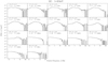 |
Fig. A.1. Average PSDs of 1−10 keV band (LE) in different spectral states. Each PSD is the average of all n PSDs falling within the given Γ1 interval. We also denote the total exposure time T in GTIs for each Γ1 interval. |
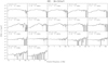
All Tables
All Figures
|
Fig. 1. Long-term behavior of Cygnus X-1 measured by all-sky monitors MAXI and Swift-BAT. We follow the same approaches of state definition proposed by Grinberg et al. (2013). Upper panel: the hard, intermediate, and soft states are denoted by blue, purple, and red points, respectively. Lower panel: the unclassified and soft states are plotted with black and red points, respectively. The duration of HXMT observations on Cygnus X-1 is shown in dark orange stripes at the top. |
| In the text | |
|
Fig. 2. HID of Cygnus X-1 using the data from three proposals: P0101315, P0201012, and P0305079, that are denoted by cyan, orange, and green, respectively. The intensity is defined by the photon count rate of LE ranging from 1 to 10 keV. We define the hardness as the ratio of the raw photon count rate between the 5−10 keV band and the 1−5 keV band. The time resolution is set to 60 s. |
| In the text | |
|
Fig. 3. Typical spectra of Cygnus X-1 with HXMT observations. Upper panel: a spectrum in the hard state (obs ID: P0201012171). The spectrum in the lower panel: is in the soft state (obs ID: P0101315057). Data from the LE, ME, and HE telescopes are denoted with black, red, and blue crosses, respectively. The power-law continuum, the thermal component, and the iron line emission are indicated with dashed lines. |
| In the text | |
|
Fig. 4. Soft photon index Γ1 of bknpower obtained by free column densities versus the obtained column densities NH during the absorption. The black dots indicate the NH obtained by the spectral fitting down to 2 keV; while the red dots indicate the NH obtained down to 1.5 keV. The dashed line represents the value 7.1 × 1021 cm−2, which is adopted during our spectral fitting. |
| In the text | |
|
Fig. 5. Histogram of the reduced χ2 over the best fits of the 145 spectra. Most of the |
| In the text | |
|
Fig. 6. Spectral evolution versus the soft photon index Γ1. Top panel: correlations of the 5−10 keV/1−5 keV hardness versus Γ1. We define the hard state (HS), the hard intermediate state (HIMS), the soft intermediate state (SIMS), and the soft state (SS) with Γ1 values. Middle panel: ratio of unabsorbed energy flux of the disk components over the total energy flux versus Γ1. Bottom panel: intensity of reflection that is denoted by the equivalent widths of the iron Kα lines, and is stronger in the soft state than in the harder state. |
| In the text | |
|
Fig. 7. Upper panel: soft photon index Γ1 versus the hard photon index Γ2 in model bknpower. The dashed line indicates that Γ1 = Γ2. Lower panel: the correlations between Γ1 and the difference of two photon indices, defined by ΔΓ = Γ1 − Γ2, are shown. The lines that are parallel to the dotted lines indicate a constant Γ2. |
| In the text | |
|
Fig. 8. The correlation of ΔΓ versus the equivalent widths of the iron Kα lines. The blue/purple/red points denote that the source is in the hard/intermediate/soft state, respectively. |
| In the text | |
|
Fig. 9. The soft photon index Γ1 of bknpower obtained by fixed NH = 7.1 × 1021 cm−2 and free NH. The dashed line indicates that Γ1 (NH fixed) = Γ1 (NH fixed). |
| In the text | |
|
Fig. 10. Correlations between the soft photon index Γ1 and the fractional rms from all the instruments on HXMT. The red circles are the raw rms without the correction of Eq. (1), and the black dots are the corrected total rms according to Eq. (1). The magenta dotted lines denote the signal-to-background ratio S/(S + B). The orange solid lines show the trends of the corrected and uncorrected total rms when varying Γ1. |
| In the text | |
|
Fig. 11. Evolution of PSDs versus the soft photon index Γ1 from different energy bands provided by all instruments on HXMT. The color scale represents the average value of PSD(fi)×fi at individual frequencies fi. Please note that the PSD values in these plots have not been corrected by Eq. (1) in order to avoid the covering effect due to the high signal-to-background ratio. |
| In the text | |
|
Fig. 12. Same as the last row of Fig. 11, but with a different color scale in order to illustrate the evolution of the variability component more clearly. |
| In the text | |
|
Fig. 13. Evolution of the coherence function γ2 and the phase-lags versus the soft photon index Γ1 between different energy bands of the LE telescope. |
| In the text | |
|
Fig. 14. Evolution of the coherence ⟨γ2⟩ averaged over the 0.0625−6 Hz frequency range versus the states (classified by the soft photon index Γ1) between different energy bands. |
| In the text | |
|
Fig. 15. Similar to Fig. 14, but with the evolution of the average phase-lag versus the states (classified by the soft photon index Γ1). In the first three panels, the average phase-lags with Γ1 ≥ 2.4 are denoted by dotted lines, as we know that the loss of coherence is due to the different emission origins. |
| In the text | |
|
Fig. 16. Average power spectra calculated from light curves obtained from the HE instrument in different energy bands in four different Γ1 ranges. The PSDs for the 30−50 keV band, 50−90 keV band, and 90−150 keV band are denoted with black, red, and blue lines, respectively. The PSDs are rebinned to df/f = 0.3. |
| In the text | |
|
Fig. A.1. Average PSDs of 1−10 keV band (LE) in different spectral states. Each PSD is the average of all n PSDs falling within the given Γ1 interval. We also denote the total exposure time T in GTIs for each Γ1 interval. |
| In the text | |
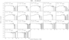 |
Fig. A.2. Similar to Fig. A.1, but for 10−30 keV band (ME). |
| In the text | |
Current usage metrics show cumulative count of Article Views (full-text article views including HTML views, PDF and ePub downloads, according to the available data) and Abstracts Views on Vision4Press platform.
Data correspond to usage on the plateform after 2015. The current usage metrics is available 48-96 hours after online publication and is updated daily on week days.
Initial download of the metrics may take a while.