| Issue |
A&A
Volume 666, October 2022
|
|
|---|---|---|
| Article Number | A123 | |
| Number of page(s) | 14 | |
| Section | Celestial mechanics and astrometry | |
| DOI | https://doi.org/10.1051/0004-6361/202243693 | |
| Published online | 18 October 2022 | |
Latitudinal dynamics of co-orbital charged dust in the heliosphere
1
Department of Astrophysics, University of Vienna,
Türkenschanzstrasse 17,
1180
Vienna, Austria
e-mail: This email address is being protected from spambots. You need JavaScript enabled to view it.
2
Department of Mathematics, University of Rome Tor Vergata,
Via della Ricerca Scientifica 1,
00133
Rome, Italy
e-mail: This email address is being protected from spambots. You need JavaScript enabled to view it.
Received:
1
April
2022
Accepted:
16
July
2022
Abstract
In recent years, observations have found evidence for dust at higher ecliptic latitudes. Different possible explanations for these signatures have been proposed, most commonly assuming that they originate from collisions of young asteroid families. In the present work, we investigate the influence of the interplanetary magnetic field causing strong latitudinal oscillations that may affect the creation and evolution of dust at these latitudes. Using numerical simulations of a charged dust particle affected by the Lorentz force, we analyse the effect of a simplified magnetic field model specifically on the long-term evolution of the orbital plane of the dust grain. Additionally, we demonstrate the significant agreement with the results of the semi-analytical secular-resonant model we have developed for charged particles in co-orbital motion with a planet. We have found that the interplanetary magnetic field determines the three-dimensional distribution of micron-sized dust grains, causing large excursions of the orbital inclination that distribute the particles to high ecliptic latitudes. The strength of these oscillations depends in particular on the particle size and on the distance to the Sun. Farther outwards in the Solar System, the particle amplitudes are larger.
Key words: magnetic fields / methods: analytical / methods: numerical / celestial mechanics / zodiacal dust / meteorites, meteors, meteoroids
© S. Reiter and C. Lhotka 2022
 Open Access article, published by EDP Sciences, under the terms of the Creative Commons Attribution License (https://creativecommons.org/licenses/by/4.0), which permits unrestricted use, distribution, and reproduction in any medium, provided the original work is properly cited.
This article is published in open access under the Subscribe-to-Open model. This email address is being protected from spambots. You need JavaScript enabled to view it. to support open access publication.
1 Introduction
The interplanetary dust cloud (IDC) is formed by interplanetary dust particles (IDPs). These are the source of scattered sunlight that is visible in the night sky and causes an astronomical phenomenon best known as the zodiacal light. IDPs are the remnants from the formation process of the Solar System. Their orbital lifetimes, however, are limited to only some thousands of years. For this reason, IDPs must constantly be produced in physical processes to maintain the IDC. Several sources have been identified. The asteroidal component is assumed to be originating from breakup events of young asteroid families (Low et al. 1984; Dermott et al. 1984; Nicholson et al. 1984), while cometary material quite probably originates from cometary activity (Nesvorný et al. 2010; Pokorný et al. 2014). Other sources may contribute to the IDC as well (e.g. circumplanetary and interstellar dust), but the relative contribution to the IDC is still under debate in the astronomical community. The IDC is known to be concentrated near the ecliptic, but observations in the infrared (COBE and IRAS) indicate the presence of fine structures, that is, dust bands and trails, at specific ecliptic latitudes. The structure of the IDC is a direct consequence of the distribution of IDPs within the Solar System, which in turn stems from the cumulative dynamics of individual dust grain orbits. Because their chaotic motion is determined by several forces that act on different timescales and magnitudes, a loss of information about their origin in space occurs with time. However, dynamical studies still enable us to constrain the possible sources and the distribution of dust grains in the Solar System.
The influence of dynamical effects on the distribution of dust has been demonstrated by the existence of dust bands in the zodiacal cloud (Espy et al. 2009). Some recent observations with star cameras on board the Juno mission (Jorgensen et al. 2021) have been claimed to confirm these dust bands as well, but disagree with existing models for the meteoroid environment in the inner Solar System (Pokorný et al. 2022). Originally, the 25 µm observations of IRAS have been used to reconstruct the density profile within ±30° in ecliptic latitude. The dust bands are found to be related to the peaks in the intensity of light that are found close to about ± 1.4°, ± 10°, and ± 17° ecliptic latitude. On the one hand, the dust bands have originally been linked to collisions of young asteroid families in the main belt (Espy et al. 2009; Sykes & Greenberg 1986; Dermott et al. 2001). On the other hand, the interpretation of some of the signatures in Jorgensen et al. (2021) is based on the combination of non-gravitational forces and the so-called Kozai-Lidov (KL) effect (Kozai 1962; Lidov 1962).
Both explanations rely on specific circumstances for the origin of the dust grains. In the former case, it is necessary to match the location of the dust bands to the asteroid families that likely produce dust via collisions. However, due to the large number of identified asteroid families, it is still an open question why some lead to the production of these dust bands but several others do not. Jorgensen et al. (2021), on the other hand, used the KL effect to explain the dust bands and assumed that the primary distribution has similar orbital parameters as Mars, resulting in agreement with the measured dust bands. This requires the influence of Jupiter as the distant third body to drive the KL effect. However, this does not seem to be the case according to Pokorný et al. (2022) because we lack evidence for a high abundance of dust originating from Mars. The results for the dynamics of these assumed particles are also inconsistent.
The purpose of the present study is to investigate the role of the interplanetary magnetic field (IMF) on the latitudinal distribution of dust grains on secular timescales that may also contribute to the dynamical evolution of dust bands outside the ecliptic. Dust in space becomes positively charged by the photoelectric effect (Lhotka et al. 2020). Orbital motions in the IMF therefore lead to a non-negligible Lorentz force term that affects the orbits of the charged particles in various ways: Lhotka et al. (2016) showed that the normal component of the IMF may affect the radial drift towards the Sun, and the destabilising effect of the IMF on particles trapped in mean motion resonances (MMR) was demonstrated in Lhotka & Gales (2019). Non-gravitational effects may also lead to an asymmetry between the location and size of the resonance locations L4 and L5 as has been shown for charged IDPs in the vicinity of Venus in Zhou et al. (2021) and of Jupiter in Lhotka & Zhou (2022). We note that these latter two studies were motivated by recent findings in Pokorný & Kuchner (2019) (for Venus) and Liu & Schmidt (2018b,a) (for Jupiter).
In the current study, however, we assume that micron-sized particles are already trapped in 1:1 MMR with a planetary perturber (primarily with either Jupiter or Venus). For our purposes of studying the influence of the IMF on the distribution of these particles, this also legitimises the neglect of further non-gravitational effects. These force terms mainly affect a and e of the dust grain. They therefore either reduce (Poynting–Robertson effect, solar wind for larger particles) or increase (solar radiation pressure for smaller particles) the solar distance (for more details on these effects, see e.g. Burns et al. 1979). Previous studies (e.g. Liou & Zook 1995) have found that particles can be trapped in MMRs for several thousand years, during which these non-gravitational forces cause little change in the orbit. In contrast to this, the Lorentz force mainly affects the orbital plane and therefore does influence particles in co-orbital motion with a planet.
The mathematical and physical background of our computations together with the set-up of the simulations and the development of the semi-analytical secular-resonant model are explained in Sect. 2. Our results are summarised in Sects. 3 and 4. In Sect. 3, we study the overall structure of the parameter space of the orbital plane and the dependences of this structure on the particle and environmental properties. In Sect. 4, we translate our results first into proper elements and second into the distribution along the ecliptic longitude and latitude. Lastly, we present discussions on the results and our conclusions in Sect. 5.
2 Mathematical models and tools
2.1 Notation and assumptions
For simplicity, we assume that the planet moves on a circular orbit in the ecliptic plane of the Solar System, which is used as the quasi-inertial system of reference for all computations. To describe the evolution of the particle’s orbital plane, it is therefore necessary to express the orbital system (eX, eY, eZ) in ecliptic coordinates (ex, ey, ez). This is done using the Kepler elements, that is, the semi-major axis a, the eccentricity e, the inclination angle i, the argument of perihelion ω, the longitude of the ascending node Ω, and the mean anomaly M of the dust grain. The object’s position vector is expressed as r = (x,y,z). As we aim to study the dynamics of a charged particle trapped in 1:1 MMR with a planetary perturber, the dust grain is positioned at either the L4 or L5 point on the planetary orbit, that is, the points of gravitational equilibrium.
Additionally, we also need to consider the orientation of the equatorial system (ex, ey, ez) with respect to the ecliptic system, as is demonstrated in Fig. 1. This is required because the IMF is included. For the solar rotation axis, which gives the ez-axis of the equatorial plane, we assume the orientation resulting from the so-called Carrington elements (ic, Ωc), which are named after Carrington (1863). ic is the inclination angle of the equatorial plane with respect to the ecliptic plane, while Ωc gives the angle between the vernal equinox and the intersection line of the two planes. This can also be inferred from Fig. 1. This work uses the values (ic, Ωc) = (7.15°, 73.5°), as found in Beck & Giles (2005).
For the structure of the IMF, we assume a time-independent, three-dimensional Parker spiral model according to Parker (1958) and Webb et al. (2010). This neglects the effect of the solar cycle but takes the dipole structure and the coiled-up field lines in the Solar System into account (see Fig. 2). The magnetic field is carried outwards in the Solar System by the solar wind (with velocity uSW). The spiral structure develops as a result of the solar rotation (with rotation rate Ωs). For simplicity, we also assume that the dipole axis of the IMF coincides with the z-axis of the equatorial plane (Fig. 1), that is, the tilt angle between these two axes equals zero; compare Lhotka & Narita (2019). Strictly speaking, this is only approximately accurate during solar minimum (Smith et al. 1978; Jokipii & Thomas 1981). However, for the aim of studying the mean effects of the IMF on the orbital planes of charged IDPs, this simplified model suffices. For the equation of the magnetic field vector B, we therefore assume
 (1)
(1)
where B0 is the constant background magnetic field at a reference distance of r0 = 1 AU and the tanh-term, parametrised by α, models the sign change of the IMF at the equatorial plane. For more details, see Lhotka & Galeş (2019). This transition region between the magnetic north and the magnetic south is referred to as the heliospheric current sheet. The Lorentz force per particle mass m caused by the interaction of the IMF with the charged dust grains can be expressed as
 (2)
(2)
where q/m is the charge-to-mass ratio. Because we assume spherical geometry of the dust grain, we can also write
 (3)
(3)
where є0 is the dielectric constant in vacuum, ρ is the particle density (here assumed to be constant, see Table 1), U is the particle’s surface electric potential, and R is its radius.
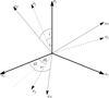 |
Fig. 1 Overview of the reference systems: ecliptic plane (thick lines), equatorial plane (dashed), and orbital frame of the particle. The dotted line represents the node line that points in the direction of the ascending node of the orbital plane. |
Parameters and symbols for the computations.
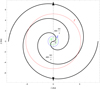 |
Fig. 2 Sketch of the coiled-up structure of the IMF. This simplified shape is shown here in the equatorial |

2.2 Simulation set-up
Two kinds of computations were made to study the effects of the IMF on charged dust grains in co-orbital motion with a planetary perturber. On the one hand, the Newton equations of motion were used for numerical simulations of the full dynamics. For this, we used the equation of motion as
 (4)
(4)
where F here represents an arbitrary external force term per particle mass and µ = GM⊙, with M⊙ as the solar mass. On the other hand, we used the Gauss equations of motion1 (using the orbital elements instead of the Cartesian coordinates) to derive the long-term evolution of i and Ω according to
 (5)
(5)
 (6)
(6)
For the influence of the perturber, we assumed a gravitational potential U1 as in Lhotka & Celletti (2015) of the form of
 (7)
(7)
where m1 is the mass of the planet and r1 = (x1, y1, z1) = (a1 cos M1, a1 sin M1, 0) is its position vector. The additional term of 1/r was included for frequency correction specifically for the case where a = a1 (i.e. n = n1), see Brown & Shook (1964).
The force on the dust grain caused by the planet can then be derived from the gradient of the potential of Eq. (7), that is, F1 = −∇U1/m, which yields
 (8)
(8)
The Lorentz force was implemented in the form of
 (9)
(9)
using Eqs. (1) in (2), as in Lhotka & Galeş (2019).
To numerically solve the Newton equations of motion, we plugged Eqs. (8) and (9) into Eq. (4) in the form of F = F1 + FL. In addition to these terms, we also need the initial conditions of the position and the velocity vector, r and  . After integration, the results were converted into the orbital elements. For the integration process itself, we used NDSolve in Wolfram Mathematica, using an explicit Runge–Kutta method of order 8 with a flexible time step. For integrations over several thousand years, we applied a constant step size instead.
2.3 Development of the secular-resonant model
While Eq. (8) can be used in Eq. (4) for the Newton solution of the gravitational influence on the particle motion, it has proven to be advantageous to start from the potential term in Eq. (7) in order to implement it into the Gauss equations. Series expansions of the terms l/||r − r1|| and  for the case of r ~ r1 in small parameters approximate the potential. In doing this, we write ρ = r/r1 − 1 and cosψ = rr1/(rr1). For more details, see also Lhotka & Celletti (2015). When the gradient of this expanded expression is implemented into the Gauss equations, a large number of terms is obtained. However, it is possible to reduce these terms to those containing only the information for the long-term evolution of the orbital elements. This was done by isolating the terms containing multiples of the so-called resonant angle Φ = ω + Ω + M − M1 from the full solution. The resulting equations for each of the Kepler elements take the form of a Fourier series, as was found in Reiter (2021). For i and Ω, we find
 (10)
(10)
 (11)
(11)
where the three orders of expansion (k, l, m) are due to the series expansions of U1, and cklm represents polynomials in e. A comparison between the full Newton solution and the Gaussian approximation is given in Fig. 3. In the simulations, we included all six equations to compute the effect of the planet on particle motion. As the expression for a, e, ω, and M are similar to Eqs. (10) and (11), we only show these two as an example.
Equations (10) and (11) now contain only the terms responsible for the secular behaviour of the orbital plane under the influence of the gravity of the perturbing planet. Similar expressions are necessary to analyse the long-term effects of the Lorentz force. Lhotka & Galeş (2019) implemented Eq. (9) into the Gauss Eqs. (5) and (6). They derived the secular equations as
 (12)
(12)
 (13)
(13)
where ez = (x0, y0, z0). In these equations, there is also a dependence on the mean motion n. Figure 4 demonstrates the agreement between the Newton solution derived from Eqs. (8) and (9) in Eq. (4) for i and Ω and the results of the combination of Eqs. (12) and (13) with Eqs. (10) and (11). As in Fig. 3, the secular-resonant model only shows the secular oscillations without the superposed higher-order harmonics. We note that the inclusion of the Lorentz force modifies the oscillations in both i and Ω significantly in comparison to what we have seen in Fig. 3, causing much greater excursions in the latitude. The preliminary results of this section indicate that the influence of the IMF acting on charged particles significantly affects their three-dimensional distribution.
2.4 Linear stability analysis
The Gauss Eqs. (12) and (13) can further be used to derive conditions for an equilibrium and to determine its stability indices (in absence of the perturbing planet). The condition is obtained by adding the second order terms in x0, y0, 1 − z0 to Eqs. (12) and (13) (taken from Lhotka & Galeş 2019) and setting both equations equal to zero. At given distance a and for fixed parameters α,  , and q/m, via division by the common factors on the left and right of the respective equations, we obtain the system of equations:
![Mathematical equation: $ \matrix{ {\left[ {{x_0}\cos {\rm{\Omega }} + {y_0}\sin {\rm{\Omega }}} \right] \times C\left( {{\rm{\Omega }},i;n,{{\rm{\Omega }}_{\rm{s}}}} \right) = 0,} \hfill \cr {\left[ {\cos i\left( {{y_0}\cos {\rm{\Omega }} - {x_0}\sin {\rm{\Omega }}} \right) + {z_0}\sin i} \right] \times C\left( {{\rm{\Omega }},i;n,{{\rm{\Omega }}_{\rm{s}}}} \right) = 0,} \hfill \cr {C\left( {{\rm{\Omega }},i;n,{{\rm{\Omega }}_{\rm{s}}}} \right) = n + {{\rm{\Omega }}_{\rm{s}}}\left[ {\sin i\left( {{y_0}\cos {\rm{\Omega }} - {x_0}{\rm{sin\Omega }}} \right) - {z_0}\cos i} \right].} \hfill \cr } $](/articles/aa/full_html/2022/10/aa43693-22/aa43693-22-eq18.png) (14)
(14)
Setting both equations to zero and solving for i and Ω allows us to locate the equilibrium positions. Setting x0 cos(Ω) + y0 sin(Ω) = 0, we have x0/y0 = − tan Ω and the corresponding system
 (15)
(15)
Using the definitions x0 = sin ic sin Ωc, y0 = − cos Ωcsin ic, z0 = cosic that locate the magnetic pole in terms of Ωc, ic in the inertial frame of reference, we find from Eq. (15)
 (16)
(16)
with the solution Ω* = Ωc, i* = ic. Thus, the equilibrium of Eq. (14) is given when the poles of angular momentum are (anti-) aligned with the magnetic poles of the Sun, that is, Ω* = 73.15°, i* = 7.15° with the choice of the parameters in Table 1. We note that this equilibrium only depends on the geometry of the problem, that is, the choice (Ωc, ic). The Jacobian matrix of the vector field defined by Eqs. (12) and (13) expanded around (Ω, i) = (Ωc, ic) becomes
 (17)
(17)
with eigenvalues  . As a conclusion, the equilibrium Ω* = Ωc, i* = ic is a neutral centre for all parameter ranges.
In addition, the condition (14) is fulfilled for any choice of (Ω(0), i(0)) such that C(Ω0, i0; n, Ωs) = 0. For vanishing x0 and y0, the condition is fulfilled for i close to 90°. To first order in i expanded around i = π/2, we find the approximate solution
 (18)
(18)
No closed-form solution of the eigenvalues of the Jacobian for initial conditions (Ω0, i0) that satisfy C(Ω0, i0, n, Ωs) = 0 could be found. However, substitution of numerical values for the parameters indicates zero eigenvalues of the Jacobian in all cases. From a numerical point of view, equilibria that satisfy C(Ω0, i0, n, Ωs) = 0 turn out to be unstable. We call the equilibrium that satisfies Eq. (15) the (pure) geometric, and pairs (Ω0, i0) that fulfill C(Ω0, i0, n, Ωs) = 0 unstable steady-state solutions from now on. We note that the latter, in addition to the geometry of the basic reference frames, also depend on the ratio n/Ωs, and stable configurations in the parameter space might exist. However, in the following, we restrict our analysis to the neutral equilibrium, while the other equilibria will be investigated in a separate study.
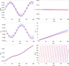 |
Fig. 3 Results of the numerical simulations using the Newton equations (blue) and the resonant Gauss equations (red). This comparison shows the evolution of the orbital elements of uncharged dust grains in co-orbital motion with Jupiter. |
2.5 Basic periods and computations
It is necessary to differentiate between several terms referring to a period when we discuss the variations in i. For the long-term oscillations resulting from our model (see Fig. 4), we use the term secular period (typically on timescales of a few hundred years). The higher-order harmonics (which are only found in the full dynamical solution) superposed on this mean oscillation yield variations on shorter timescales of a few dozen years. These are hence also referred to as the short-period oscillations. Additionally, we further also use the term orbital period to describe the particle as it moves on its orbit in Sect. 3.3.
In order to discuss the results of different simulation runs, we primarily compare the secular periods and amplitudes of the i-oscillations in the following sections. This is done to evaluate the induced latitudinal variations for different particle properties and initial conditions. We use the two different methods for the different approaches (Newton and Gauss) and compare different data sets to validate the results. In the case of the Newton equations, we use a function to derive the position of the maxima by computing the time step at which Ω ~ Ωc (at which we find an extremum in i, compare Sect. 2.4). This was done twice to be able to calculate one full oscillation period by subtracting the time step of the first maximum t1 from the second t2. The uncertainty in this method of period computation was estimated using
 (19)
(19)
where tmin is the time step corresponding to the minimum. This value was found by simply locating the minimum value of i in the computed interval. For each result, σ was used to estimate the variation in the derived period length.
As the Gauss equations compute only the secular parts of the oscillation, the resulting function is much smoother without the higher-order harmonics. We therefore used the function FindPeaks implemented in Wolfram Mathematica to locate the first two maxima in the oscillation of i. This again allowed us to compute the period length. The minimum was found in the same way as in the Newton case, and the uncertainty was similarly computed by Eq. (19).
The amplitudes were derived in the same way in both approaches: by subtracting the minimum from the maximum value in i in the integrated interval. Due to the additional higher-order harmonics in the full dynamical solution, the amplitudes of the Newton computations are slightly larger (typically by up to roughly 1°).
To derive the period lengths and amplitudes of the higher order harmonics, we also used the FindPeaks function, which now located the local maxima of the smaller variations. Similarly, the minima were located by applying this function after inverting the results of the latitudinal variations. The period length of the higher-order harmonics was taken as the mean of the difference of consecutive maxima. As these oscillations are stretched and compressed over the course of the secular evolution, we also took the mean of the subtracted values of consecutive minima and maxima to derive the mean amplitude value.
In the comparison of the Newton and Gauss results in Fig. 4, an adjustment of the α-parameter was required. Equations (12) and (13) display a direct proportionality to α, but the Lorentz force in Eq. (9) does not. This is due to the expression of the tanh-term in the two Gauss equations, as it was written in the form of Lambert’s continued fraction (Lhotka & Galeş 2019). It is therefore not possible to use the same value of a in these two sets of equations.
As the tanh-term in Eq. (9) represents the sign change at the heliospheric current sheet, we used α = 100 in the Newton runs. This was also done in Lhotka & Galeş (2019), as higher values of a more accurately model an instantaneous change, that is, a thinner current sheet. This is demonstrated in Fig. 5. Due to the direct proportionality in the Gauss equations, however, the same a-value cannot be used here. It was therefore necessary to adjust the parameter in Eqs. (12) and (13) to find conformity with the Newton results. As α in the Gauss expression (αG) changes the period length of the oscillation, it is possible to do this adjustment by eye. However, the process can be automated as well. Firstly, we performed one simulation run with the Newton equations of motion with αN = 100. Then, the same set of initial conditions were used in the Gauss equations, using an arbitrary αG-value, for example 8, as was done here. The period lengths Pres and Pnewt of these results were then compared and the ratio was multiplied with αG as in
 (20)
(20)
to compute the adjusted value αG,new.
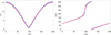 |
Fig. 4 Comparison of the oscillations in i (left) and Ω (right) between the Newton solution (blue) and the secular-resonant model (red) for the combined effect of Jupiter and the IMF. |
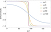 |
Fig. 5 Sketch of the function of the tanh-term in Eq. (9) in modelling the transition region between the magnetic north and south. a models the broadness of the heliospheric current sheet. |
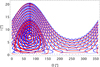 |
Fig. 6 Dynamics in the i-Ω-parameter space. We compare the results of the Newton equations (blue) and the secular-resonant model (red). |
3 Structure of the i-Ω-space
3.1 Combined effect of the IMF and the planet
In order to study the dynamics of the orbital motion, it is beneficial to analyse the results in the i-Ω-parameter space. Figure 6 shows the results of 20 simulation runs for the full Newton solution and the Gaussian model on the example of Jupiter as the perturbing planet. The initial inclination i0 was varied in the range of [1, 20]°, while Ω0 = 73.5°. The Ω-condition of the geometric equilibrium solution (of the Lorentz force) was therefore fulfilled, according to Sect. 2.4. We note that this can be identified in Fig. 6 at i ~ 7°. Rather than an exact equilibrium, the orbital plane displays a minimum amplitude oscillation due to the influence of the planet. These oscillations are very small in the case of the Gaussian results.
As Fig. 4 also showed, the Gauss equations yield only the secular oscillations in i and Ω, while the Newton solution results in the full dynamics including the higher-order harmonics. These higher-frequency variations are faster oscillations caused by the particle’s orbit around the Sun. This is studied further in Sect. 3.3 for the isolated effect of the IMF, where we place the dust grain at different solar distances, altering its orbital period in turn.
Generally, Fig. 6 demonstrates that the behaviour of the orbital planes is separated into two regimes of motion, namely a librational and a rotational regime. The orbits with initially lower inclinations up to i0 = 14° display librational behaviour, as Ω only oscillates between lower values in the range of [10, 120]°. For particles on initially more highly inclined orbits (i0 ≥ 15°), we find rotational motion, that is, Ω passes through all possible values. Additionally, Fig. 6 also shows that the maximum inclination is always reached when Ω = 73.5°. More generally speaking, this means that the orbital plane of the dust grain reaches the largest excursion in its inclination when the ascending node is aligned with the node of the intersection line of the current sheet and the ecliptic plane.
Placing the initial condition of Ω at Ωc allowed us to study the different types of orbits resulting from a range of initial inclinations. However, upon analysing the phase-space of Fig. 6, we can infer that not all values for Ω result in both librational and rotational motion. Figure 7 demonstrates this for a range in Ω of [0, 75]° in intervals of 15°. Similar to the results in Fig. 6, the initial inclinations range between 1° to 20°.
The left panel of Fig. 7 shows the change in the secular period length of the i-oscillation (as defined in Sect. 2.5), indicating that the inclination varies faster when the ascending node is more closely aligned with the heliospheric current sheet. Additionally, it is apparent that the period lengths in dependence of the initial inclination display a V-like shape for Ω0 ≥ 15°. For lower Ω0 values, the periods increase continuously for higher i0. This is connected with the changes in the inclination amplitudes for different Ω0, shown in the right panel of Fig. 7. Here, the type of motion in the i-Ω-space changes, a transition from librational to rotational motion. This is seen most clearly for Ω0 ≥ 45°. The transition occurs at around 14° for Ω0 = 75°, as is also inferred from Fig. 6 for Ω0 = Ωc.
Upon comparing the results for the two Lagrange regions L4 and L5 (Φ = 60° and Φ = 300°, respectively), we note that there does not appear to be any difference in the results between the two regions (not shown here, but can be seen in Reiter 2021) for Jupiter and Venus. This indicates that the placement of the dust particle relative to the planet does not seem to cause significant differences in i-Ω-space. We would therefore expect dust grains of both regions to display a similar vertical distribution. In parallel, the results for simulations of a tadpole and a horseshoe orbit (not pictured here) yield comparable results. The similarity between the different types of orbits further supports the assumption that the IMF is the dominant factor influencing the particle motion in the i-Ω-space.
3.2 Effect of the charge-to-mass ratio
A change in the surface electric potential U and the radius R of the particle in Eq. (3) leads to a variation in the strength of the Lorentz force. These simulations help to constrain possible limitations for our simplified secular-resonant model. Much like in the variation in Ω0 in Fig. 7, we cover the i0 range of [1, 20]°. For the comparability with the parameter space of Fig. 6, however, we assumed that Ω0 of each particle orbit was located at the intersection line of the equatorial and the ecliptic plane (i.e. in the heliospheric current sheet, Ω0 = Ωc).
First, U takes values from 0.5–5V at a fixed particle radius of R = 2 µm. These results are shown in Fig. 8. The values for the secular frequency and the amplitudes both indicate higher inclinations when U = 5 V, which corresponds to the strongest influence of the Lorentz force. This means that the latitudinal variations of IDPs occur faster on average for higher charge-to-mass ratios, also leading to slightly higher (of about 1°) ecliptic latitudes than for 0.5 V.
The same general effect is seen for the results of the variation in particle size that is provided in Fig. 9. The dust grain radius was varied in the range of [1, 10] µm at a fixed surface potential of U = 5 V. As the particle size appears with a factor of R−2 in (3), it influences the charge-to-mass ratio more strongly than U, which is also evident from comparing the results in Figs. 8 and 9. We again note the increasing frequency and amplitudes for higher q/m values (that is, smaller particle sizes) but there is also a strong change in the trend in both results. The right panel of Fig. 9 demonstrates that for particle sizes of about 1 µm, the common V-shape found on the right of Fig. 8 and in the Ω0 = 75° case on the right of Fig. 7 in the results of the amplitude disappears, indicating a loss of the structure in the i-Ω-space consisting of the librational and the rotational regime. Similarly, the results for the period function (left panel of Fig. 9) show the largest variation for R = 1 µm. This indicates that the oscillation of i is no longer regular in this case and even less so for smaller dust grains. It is important to note that the other non-gravitational forces, in addition to the Lorentz force, become increasingly more important for sub-micron particles (see e.g. Kimura & Mann 1999). This is especially the case for the solar radiation pressure, which effectively removes the particle from the resonance early on, as it destabilises the resonance (compare e.g. Liu & Schmidt 2018b). Hence our results would no longer be directly applicable in these cases. Out of academic interest, however, we also studied the resulting i-Ω space for dust grain sizes of 0.5 µm and 0.7 µm, as we wished to analyse the destruction of the phase space solely due to the interaction of the charged submicron sized particles with the IMF. This destruction is already suggested in the threshold case (i.e. 1 µm) in Fig. 9. The results for the two sub-micron cases (not pictured here) again highlight the loss of structure evidenced by the lack of distinction between librational and rotational orbits. This is especially the case for the 0.5 µm particle, where evidence for librational motion is no longer found. Incidentally, the i0 = 7° simulation run shows the largest amplitude, meaning that we no longer find a minimum amplitude solution close to the geometric equilibrium due to the strong effect of the IMF. While in reality, dust grains with sizes smaller than about 2 µm (Liou & Zook 1995) would be displaced from the resonance early on due to the solar radiation pressure, we find that even the stronger effect of the IMF alone would also lead to irregularities in the variation of the inclination, as shown in Fig. 9 by the 1 µm case. In a more realistic set-up, dust grains of this size would not remain trapped in resonance for long because of the destabilising effect of the solar radiation pressure. In a direct follow-up paper to our current study, we are working on incorporating solar radiation pressure and the Poynting–Robertson and solar wind effect into the model.
We set the applicability of the secular-resonant model to particles of sizes R ≥ 2 µm. The motion of particles with radii smaller than this value cannot be computed accurately with the Gaussian model. This is due to the loss of periodicity for the i oscillation of smaller particles due to the increased strength of the IMF influence. The Gauss equations were derived from the assumption of particles moving on perturbed Keplerian orbits due to the dominant influence of the solar gravity. The forces causing these perturbations, however, were assumed to be less significant than the gravitational force exerted by the Sun. This is apparently no longer the case for the particles of sizes <2 µm in our simulation set-up. In these cases, the dominant force term is the Lorentz force (and the other non-gravitational forces). This also agrees with the results in Fig. 1 of Lhotka & Galeş (2019). The effect of this force can no longer be reproduced with the Gauss equations. Hence, the model can only be applied for particles ≥2 µm in the case of U = 5 V. An upper limit for the dominance of the IMF cannot be set as easily using the osculating elements. Transforming the results into proper element space allows us to analyse the proper frequencies in i and to study the changes as the influence of the IMF decreases with larger R, as we discuss in Sect. 4.1.
The results in i-Ω space (Fig. 6) and the derivation of the extrema from the secular equations (see Sect. 2.4) of the Lorentz force, indicate that the maximum excursion in latitude occurs when the ascending node of the orbital plane coincides with the intersection line of the heliospheric current sheet and the ecliptic. From the results of this parameter study in R, it appears that the maximum amplitude reaches approximately 15° for particle sizes of R > 1 µm (compare the right panel of Fig. 9).
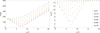 |
Fig. 7 Changes in the secular period (left) and amplitude (right) in the latitudinal variations for different Ω0 and i0 values. |
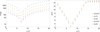 |
Fig. 8 Secular period (left) and amplitude (right) of the oscillation in i for different surface electric potentials U at a fixed dust grain size of R = 2 µm. |
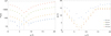 |
Fig. 9 Results for latitudinal variations for different particle sizes R at a fixed surface potential of U = 5 V. The 1 µm example marks a threshold case (see text). |
3.3 Effect of the solar distance
The results discussed so far have all been shown for the system of a dust grain in co-orbital motion with Jupiter. The parameter study was made in the same manner for a particle near Venus, and the results agree from a qualitative point of view. The main differences between the two cases are found in the shorter secular period lengths in the case of Venus and in smaller differences in the amplitudes between different values of q/m (in comparison to the variations of up to 2° we found e.g. in Fig. 8). Additionally, while we find a loss of structure in the i-Ω space for Jupiter already for particles of R ≤ 1 µm, this value shifts to slightly lower values for Venus. This results in smaller amplitudes in i for the R = 1 µm simulation as compared to the right panel of Fig. 9 and hence in a slight shift of the applicability of the secular-resonant model to 1 µm for particles near Venus. In order to investigate whether these effects are due to the different planetary influence or to the shorter solar distance, we studied the effects separately. For this purpose, it is informative to study the isolated effect of the IMF on charged particles to analyse how it affects the particle motion at different distances a0. Figure 10 shows the results for both the secular and the short-period oscillations for the variation of i in the case of a particle with i0 = 20°. The oscillation frequencies of both decrease further outwards in the Solar System, while the amplitudes increase.
This initially seems contradictory, as the strength of the IMF decreases with solar distance (the induced variations from the initial value should be smaller, i.e. result in smaller amplitudes). However, as the bottom left panel of Fig. 10 demonstrates, the mean period lengths of the higher-order harmonics coincide with the orbital period of the particle at the given solar distance. This indicates that these oscillations arise because the polarity reversal occurs twice for each orbit. When the particle crosses the heliospheric current sheet, the IMF acts on it with equal strength, but in the opposite direction, likely causing the short-period oscillations. Because the orbital period is longer for a higher semi-major axis value, this means that the dust grain is affected by the Lorentz force for a prolonged period of time in one direction before the sign change occurs. Hence, despite the overall weaker effect of the Lorentz force, the particle reaches higher ecliptic latitudes during this time before its motion is reversed.
This also results in high amplitudes overall, as shown in the upper right panel of Fig. 10. Additionally, the two panels on the right of Fig. 10 also show the result for a line resulting from the best fit from the data points using the Fit-function in Wolfram Mathematica. Interestingly, the slope of the evolution along the semi-major axis is similar for the latitudinal amplitudes for the secular oscillation and the higher-order harmonics, with a value of about 0.15 deg/AU.
4 Proper frequencies and ecliptic latitudes
4.1 Proper elements
As we focus on the evolution of the orbital planes, we used the p–q-parameter space (e.g. Morbidelli 2002) formed by i and Ω with
 (21)
(21)
We note that it is also possible to study the dynamics in h–k proper element space, which consists of the eccentricity and the longitude of perihelion. However, simulations showed that no significant change is found in h-k space with varying IMF strength outside of stronger higher-order harmonics at small R. This was expected, as the Lorentz force dominates in the orbital plane of charged dust grains, while the other orbital parameters remain largely unaffected. Both e and ω are mostly affected by the gravitational influence of the planetary perturber, which is still comparatively small for micron-sized dust grains.
The difference between the osculating and the proper element representation of the results is shown in Fig. 11. Strictly speaking, the approximation of the proper elements we used was the proper radius ip and the angle Ωp resulting from
 (22)
(22)
 (23)
(23)
While i shows larger variations, ip is a quasi-constant of motion. Additionally, Ωp passes through all possible values of [0, 360]°, while Ω only oscillates between lower values in the example of Fig. 11. This also shows the difference of librational motion in the two parameter spaces. Libration in the osculating elements translates into rotational motion in the proper element space (see also Beaugé & Roig 2001). The proper frequency Ωp,f can then be derived from one full cycle in proper element space or it can be approximated from the integration by subtracting two adjacent Ωp values and dividing them by the size of the time interval between them. This was done especially for the cases without a fully computed cycle and resulted in an estimate for the instantaneous frequency during the start of the oscillation, rather than the full secular frequency, as is the case for the complete orbits in the p–q space. Figure 11 also shows a displacement of the dynamics in p-q space from the origin. This is due to the influence of the IMF or, more specifically, to the orientation of the dipole structure. In cases of a strong influence of the Lorentz force, the origin is displaced by the angles ic and Ωc.
Studying the proper element space for differently sized particles at various positions in the Solar System allows analysing the dominance of the IMF on particle motion in more detail. As mentioned in Sect. 3.2, we aim to place an upper limit on the particle size at which the influence of the IMF and of the perturbing planet become comparable in size. The left panel of Fig. 12 indicates that the influence of Jupiter becomes dominant at a particle size of about 400 µm for i0 = 5°. However, the right panel of Fig. 12 shows that the value for the proper frequency also depends on the initial inclination. For larger i0 (here i0 = 10° as an example), the proper frequency due to Jupiter is higher, while the effect of the IMF seems to be comparable. Hence, we note that the upper limit is rather set at R = 200 µm. This roughly corresponds to the particle size at which the trend in the slope of the proper frequency changes and starts to converge with the proper frequency of Jupiter in simulated i0 cases in the right panel of Fig. 12. We note that this is not an upper limit for the applicability of the secular-resonant model itself (as opposed to the lower limit we found for R in Sect. 3.2) because it does include the gravitational influence of the planetary perturber and can hence reproduce the dominant influence of the planet for larger particles as well (not pictured here).
From the upper left panel of Fig. 10, we expected the period length of the oscillation in i (and hence also in Ω) to be shorter in the case of a particle near Venus, also suggesting a higher proper frequency in comparison to the results of the Jupiter-orbit simulations due to the closer proximity to the Sun. Computations of Ωp,f for the particles along Venus’ orbit agreed with this assumption. Hence, a change in the solar distance seems to result in a vertical shift of the proper frequency. We note that the results of Ωp,f in Fig. 12 yield the result of the instantaneous proper frequencies for larger R, as in these cases, the cycle in the proper element space is not completed within the set integration time of 5000 yr. In order to determine a more exact evaluation of the mean Ωp,f value over one complete orbit in this parameter space, we also performed a few simulation runs computing a full orbit in all cases. For the first set of simulations, we focused on the isolated effect of the Lorentz force on objects in a size range of [1, 5000] µm. Additionally, the dust grains were placed at the locations of the two planets for the individual simulation runs. In agreement with the preliminary results for the comparison of the Jupiter and Venus run, Fig. 13 shows a shift in proper frequency to lower values at greater distances. The slope, on the other hand, is the same in all cases.
In order to validate the results, we moreover used analytical means to compute the proper frequency Ωp,f. The frequency of the oscillation caused by the IMF as the parameter Γ is given in Lhotka & Galeş (2019) in the form of
 (24)
(24)
Again, the α-parameter works as a multiplicative factor, but it is possible to recreate the slope of the change in Ωp,f with the particle radius R. The results of Eq. (24) also reproduce the shift of Ωp,f at a given R at different distances a0, which we have already found in the simulation runs (compare the dashed lines in Fig. 13). From the figure, we infer that the intersection between the shaded area and the dashed lines coincides with the change in the dominant force term evident from the numerical simulations, placing the upper limit in R for the dominance of the Lorentz force at about 1000 µm in the case of Jupiter and at a slightly higher value in the case of Venus.
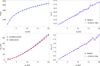 |
Fig. 10 Results for the secular oscillations of i with respect to a0 (upper panel), and results for the higher-order harmonics (lower panel; subscript “hoh”). The initial conditions are always set to i0 = 20° and Ω0 = 73.5°, and U and R from Table 1. All results are derived from the Newton set of equations. |
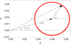 |
Fig. 11 Relation of osculating and proper elements (i and Ω vs. ip and Ωp). |
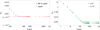 |
Fig. 12 Approximated mean proper frequencies (°/yr) for a range of particle radii R (left: for i0 = 5°). We also compare the results for two i0 values (i0 = 5° and i0 = 10°) for possible dependences on i (right). |
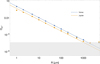 |
Fig. 13 Proper frequency Ωp,f [°/yr] resulting from the isolated influence of the IMF at different solar distances of the particle (dashed lines). The dots correspond to the estimates derived from numerical simulations including the Lorentz force and the perturbing planet. |
4.2 Ecliptic longitude and latitude
We also converted the osculating elements into ecliptic longitude l and latitude b values. For this, we used the results of the Newton equations in Cartesian coordinates with equations

resulting in
 (25)
(25)
Figure 14 shows the results of this conversion for five different particle sizes with i0 = 5° as an example (for an integration time of 300 000 yr). The smaller particles reach higher ecliptic latitudes, which is what we had already expected from the results of Fig. 9. The 400 µm and 600 µm particles behave similarly to each other. Again, this fits with our expectations, in this case from Fig. 13, as the evolution of their orbital plane is increasingly determined by the influence of Jupiter rather than by that of the Lorentz force. In these cases, the dust grain does not reach ecliptic latitudes exceeding the initial inclination value. Similarly, for a dust grain with an initial inclination of 1° (not pictured here), the ecliptic latitudes of the particles of larger R only oscillate between ±1°. Nevertheless, the smaller particles between 1 µm to 10 µm do again reach latitudes of 13° and more. As in Fig. 9, the smallest case of 1 µm would likely not be found in reality, as the solar radiation pressure removes dust grains of this size and smaller very early on. We note that these particles also quickly reach their maximum excursion in the inclination. However, these high-latitude signatures would not be located within the resonance for more than a few years.
Additionally, Fig. 14 models the results for a cloud of particles for which the longitude of the ascending node precesses with time. This process in combination with the latitudinal variations might contribute to the formation of dust bands. We are currently working on investigating this hypothesis in more detail. At the current state of our investigations, the values for the ecliptic latitude vary due to the motion of the particle along its orbit rather than due to the influence of the IMF for larger particles (here represented by the 600 µm dust grain for the Venus and the Jupiter case). As a result of the smaller oscillations (and longer oscillation periods, compare e.g. Fig. 9), we find a significant difference in the ecliptic latitude values that are reached by particles of some microns and several hundred µm after short integration times. For longer integration times, moderately sized dust grains, here ranging between 10 µm to 200 µm, also result in signatures at high ecliptic latitudes. From Fig. 14, we infer that these values are more similar to the smaller particles in the case of Venus, while the difference between the 10 µm and 200 µm case is noticeable for the particle starting near Jupiter. A thorough analysis of these effects (the dependence on integration time, particle size, planet mass, and solar distance) are subject to the follow-up study of this work.
From the results of this simplified case of a charged particle trapped in co-orbital motion with a planet, we infer that while the predominant accumulation of dust in the vertical direction (especially of particles larger than some hundred µm) seems to be due to the initial inclination value of the grain, electromagnetic effects cause the particle to reach higher ecliptic latitudes. This makes it probable that we would also find (likely fainter) signatures of dust at higher latitudes as well. From our results, we would expect another accumulation of dust to occur at around 10 deg ± some degrees depending on the initial inclinations of the particles (these values seem to be reached for Venus and Jupiter), with eventually decreasing latitudinal values for larger objects. Alternatively speaking, if strong dust signatures are found at about 5° for example, as in Fig. 14, we would expect that the smallest particles of this dust population also reach higher ecliptic latitudes due to the interaction with the IMF. We would therefore not need to understand structures at higher ecliptic latitudes as new dust populations of different origins or due to external effects driven by the gravitational influence of another planet farther away, but rather as a natural byproduct caused by the Lorentz force in the Solar System.
Transformation of the results of the secular-resonant model into the values for the ecliptic longitude and latitude using Eq. (25) after conversion of the Kepler elements into Cartesian coordinates results in a good approximation of the real distribution (not pictured here), as was to be expected from the significant agreement in the i-Ω parameter space (i.e. Fig. 6). Interestingly, this is also the case without an adjustment of α in the Gauss equations. It is therefore possible to use the secular-resonant model by itself to estimate the vertical distribution of dust grains (larger than ~1 µm for reasons discussed in Sect. 3.2).
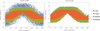 |
Fig. 14 Distribution along the ecliptic longitude l and latitude b for particles of different sizes for the case of co-orbital motion with Jupiter and Venus. l is randomly shifted to display the effect of particles at different longitudes. The 1 µm example again marks a threshold case; see text. |
5 Discussions and conclusions
We have studied the evolution of the orbital plane of spherically symmetric, charged, micron-sized dust grains trapped in co-orbital motion with a planet (specifically, the cases of Venus and Jupiter). For simplicity, we have assumed that the planet moves on a circular orbit within the ecliptic plane of the Sun, while the dipole axis of the time-independent magnetic field model is co-aligned with the rotation axis of the Sun. This assumption allowed the use of the equatorial coordinate system to describe the orientation of the IMF, placing the heliospheric current sheet within the equatorial plane. This transition region was assumed to be flat, leading to an instantaneous passage from the magnetic north into the magnetic south. Because the particle is trapped inside 1:1 MMR with the planet (and may remain this way for several thousand years), we only included the perturber’s gravitational influence and the Lorentz force.
We have found that the interaction between the charged dust grain and the IMF dominates the long-term behaviour of the particle’s orbital plane, which in turn determines its three-dimensional distribution. The Lorentz force acting on these charged particles causes large latitudinal variations, especially for objects with sizes of some µm (Figs. 9 and 14). Depending on the initial values of both i and Ω, we find two separate regimes of motion in the parameter space of the orbital plane: Low initial inclinations up to 14° and an ascending node initially located between 10° to 120° result in librational behaviour. Higher values yield rotational motion in i-Ω space (Fig. 6). For particle orbits that initially were aligned with the heliospheric current sheet, we find a minimum amplitude libration.
Figure 14 has shown that the Lorentz force can distribute the dust grains to higher ecliptic latitude values than their initial inclination value suggests, making electromagnetic transport a potential candidate that contributes to the vertical structure of dust in the Solar System. The results from this figure have indicated a particle size-dependence on the latitudinal distribution of co-orbital dust grains. Additionally, as the period length of the variation of the orbital inclination is longer for larger particles (as is indicated in Fig. 9) and they hence reach their maximum inclination value later, we also expect a dependence on the time since the dust grains were created (i.e. different amounts of dust at high latitudes depending on whether it was produced a few hundred or a few thousand years ago). Based on the differences in Fig. 14 between the Jupiter and Venus cases, we further expect a dependence of the distribution on planet mass and solar distance. These effects are subject to a more detailed follow-up study. We found these promising results from our simplified study of a single charged particle in co-orbital motion with Jupiter and Venus. The effects can also be recreated using our secular-resonant model without adjusting the a-parameter to estimate the maximum ecliptic latitudes reached for the different particle sizes. For an evaluation of the contribution of electromagnetic transport to the vertical structures found in observations, further detailed investigations into the effect are required that also incorporate the other non-gravitational forces, as well as a study of the strength of this effect on particles outside of resonance. We are currently working on implementing these points into our follow-up study. We also plan on further expanding these simulations to resemble a more realistic system by implementing an initial dust population and a more realistic magnetic field model in the future.
The main role of the resonance is to lock the particle into place, causing it to be trapped at a specific distance to the Sun. This allows the IMF to alter the particle’s orbital plane over a prolonged period of time, resulting in higher ecliptic latitudes. For an initially evenly distributed IDC, we would therefore expect an eventually more widely spread distribution of the dust grains in the vertical direction at the location of the resonances. Outside of resonance, both a and e of the particle continuously change due to the additional forces. Depending on its size, the dust grain may either be carried outwards of the planetary system or dragged inwards towards the Sun. This inwards drag can take between some hundred and thousand years depending on R, see e.g. Koschny et al. (2019). Hence, the variation in particle inclination would therefore likely not show the same amplitude at all times, but its period length and amplitude would instead evolve along the trend shown in Fig. 10. For a dust grain wandering inwards in the Solar System, this likely means that its ecliptic latitude may diminish over time. In this study, we assumed that the particle is already locked in place because capture into the 1:1 MMR is still an open question due to the inefficiency of resonant trapping in these regions (compare e.g. Liou & Zook 1995). Possible sources for such particles injected into the resonance are the Trojan asteroids on the Jupiter orbit (see e.g. Liu & Schmidt 2018a). For the case of Venus, Pokorný & Kuchner (2019) proposed that an undetected population of asteroids may be locked in 1:1 MMR with the planet that supply the area around Venus with dust.
We used the simplified version of the IMF in the shape of a dipole field, rather than its more complex structure. As we further assumed that the dipole axis of the IMF is aligned with the rotation axis of the Sun, the tilt angle in our case was zero. According to Jokipii & Thomas (1981), this is only the case at solar minimum, and even then only approximately. As we used a time-independent magnetic field model, this is a valid assumption. In reality, however, the tilt angle varies due to the solar activity. The combination of this effect with the solar rotation results in a wavy heliospheric current sheet and not in a flat transition region. This means that we do not necessarily find a cohesive structure above and below the solar equator, but rather different ‘sectors’ between which the sign of the IMF varies (see e.g. Lhotka & Narita 2019). This suggests that we likely would not find orbital planes in an equilibrium position because the shape of the heliospheric current sheet would no longer be flat, as there would no longer be a pure geometric steady-state solution.
In order to discuss the validity of our results, we considered what we would expect for the results if we were to include the alternating sign change due to the solar cycle. As the bottom left panel in Fig. 10 has shown, the periods of the higher-order harmonics correspond to the particle’s orbital period at a given distance to the Sun. During one full period, the particle therefore crosses the magnetic equator twice, which means that the shape of these oscillations is superimposed on the secular variation. Out to around 5 AU, this oscillation period is shorter than (or comparable to) the length of the solar cycle. For dust grains at greater distances than this, the magnetic field B would change its sign before one full orbital period would be completed. Test simulations using a negative B0 value result (not pictured here, but shown in Fig. 5.1 in Reiter 2021) in a reversed motion in i–Ω space. This is noticeable in the orientation because it changes from clockwise (as in Fig. 6) to counterclockwise. This means that the initial change in Ω changes from ascending to descending. Additionally, we note that the maxima and minima are interchanged. The overall shape of the secular oscillation in the parameter space does not change, however. Similar tests with the Gauss set of equations, Eqs. (12) and (13), have shown this. We therefore assume that it would be possible to recreate the effect of the solar cycle with these equations as well if the term for the Lorentz force, Eq. (9), were adapted accordingly, as was done in Lhotka et al. (2016), for example. We showed here that periodic variations in the background magnetic field strength lead to additional variations of the orbital elements of charged dust, as expected. In addition, non-zero normal force components of the IMF may trigger secular variations in orbital distance, that is, in the evolution in time of the semi-major axis. Hamilton et al. (1996) showed that effects dependent on the solar cycle may also lead to escape of dust from the Solar System. Different more sophisticated IMF models have also been evaluated in Lhotka & Narita (2019), including a strong latitudinal dependence of the field, a non-zero poleward component (not aligned with the rotation axis of the Sun), or a non-zero tilt angle of the magnetic axes, leading to a ballerina skirt shape of the zero current sheet. The inclusion of additional harmonics in addition to the dipole structure of the magnetic field of the Sun would result in additional sectors in which a sign reversal of the background magnetic field strength takes place. While all these models are able to reproduce specific features of the IMF, their usage for qualitative studies is rather limited because these are second-order effects, that is, they are small in magnitude in comparison with the standard Parker spiral model of the IMF. It is difficult to predict how strongly the inclusion of additional effects will alter the motion of particles in space. Most probably, second-order and time-dependent effects will lead to shifts and to a distortion of the structures in i-Ω space. This is an interesting topic for future studies in the field and is also important to better understand space weather in interplanetary space.
For the inclusion of the Poynting–Robertson and solar wind effect, and the solar radiation pressure, we would expect that the structure found in i-Ω space would remain similar to our results. The strength of the latitudinal oscillations would likely vary, however. As Fig. 10 shows, the period lengths and amplitudes change with distance to the Sun. Therefore, we would assume that the latitudinal variations would be modified, while the overall structure of i-Ω space would remain similar when the other non-gravitational forces were included in these computations. This remains to be confirmed in future work. While we argue for the likelihood of the Lorentz force as a driving mechanism for distributing micron-sized dust grains to higher ecliptic latitudes, we are therefore only at the starting point of the investigation into the effect of the IMF. We discussed our expectations of a change in the results when solar cycle effects and the other non-gravitational forces were included. These hypotheses remain to be confirmed or refuted in the future. We plan on including the time-dependency of the IMF, which will result in a more complex structure of the heliospheric current sheet. In a direct follow-up paper to this work, we will primarily focus on studying the distribution along the ecliptic plane of charged IDPs in co-orbital motion with a planetary perturber in more detail.
Acknowledgements
This work is fully supported by the Austrian Science Fund FWF with project number P-30542. C.L. acknowledges support from EU H2020 MSCA ETN Stardust-R Grant Agreement 813644 and MIUR Excellence Department Project awarded to the Department of Mathematics, University of Rome Tor Vergata, CUP E83C18000100006.
References
- Beaugé, C., & Roig, F. 2001, Icarus, 153, 391 [CrossRef] [Google Scholar]
- Beck, J. G., & Giles, P. 2005, ApJ, 621, L153 [NASA ADS] [CrossRef] [Google Scholar]
- Brown, E. W., & Shook, C. A. 1964, Planetary Theory, Dover, S1133 (Dover Publications) [Google Scholar]
- Burns, J. A., Lamy, P. L., & Soter, S. 1979, Icarus, 40, 1 [Google Scholar]
- Carrington, R. C. 1863, Observations of the spots on the sun from November 9, 1853, to March 24, 1861, made at Redhill [Google Scholar]
- Dermott, S. F., Nicholson, P. D., Burns, J. A., & Houck, J. R. 1984, Nature, 312, 505 [NASA ADS] [CrossRef] [Google Scholar]
- Dermott, S. F., Kehoe, T. J. J., Grogan, K., et al. 2001, Orbital Evolution of Interplanetary Dust (Berlin, Heidelberg: Springer Berlin Heidelberg), 569 [CrossRef] [Google Scholar]
- Espy, A. J., Dermott, S. F., Kehoe, T. J. J., & Jayaraman, S. 2009, Planet. Space Sci., 57, 235 [NASA ADS] [CrossRef] [Google Scholar]
- Fitzpatrick, R. 2012, An Introduction to Celestial Mechanics (New York: Cambridge University Press) [CrossRef] [Google Scholar]
- Fitzpatrick, R. 2016, https://farside.ph.utexas.edu/teaching/celestial/Celestial/node164.html [Google Scholar]
- Hamilton, D. P., Grun, E., & Baguhl, M. 1996, in Astronomical Society of the Pacific Conference Series, 104, IAU Colloq. 150: Physics, Chemistry, and Dynamics of Interplanetary Dust, eds. B. A. S. Gustafson, & M. S. Hanner, 31 [Google Scholar]
- Jokipii, J. R., & Thomas, B. 1981, ApJ, 243, 1115 [NASA ADS] [CrossRef] [Google Scholar]
- Jorgensen, J. L., Benn, M., Connerney, J. E. P., et al. 2021, J. Geophys. Res. (Planets), 126, e06509 [NASA ADS] [Google Scholar]
- Kimura, H., & Mann, I. 1999, in Meteroids 1998, eds. W. J. Baggaley, & V. Porubcan, 283 [Google Scholar]
- Koschny, D., Soja, R. H., Engrand, C., et al. 2019, SSR, 215, 34 [NASA ADS] [Google Scholar]
- Kozai, Y. 1962, AJ, 67, 591 [Google Scholar]
- Lhotka, C., & Celletti, A. 2015, Icarus, 250, 249 [NASA ADS] [CrossRef] [Google Scholar]
- Lhotka, C., & Gales, C. 2019, Celest. Mech. Dyn. Astron., 131, 49 [NASA ADS] [CrossRef] [Google Scholar]
- Lhotka, C., & Narita, Y. 2019, Ann. Geophys., 37, 299 [NASA ADS] [CrossRef] [Google Scholar]
- Lhotka, C., & Zhou, L. 2022, Commun. Nonlinear Sci. Numer. Simul., 104, 106024 [NASA ADS] [CrossRef] [Google Scholar]
- Lhotka, C., Bourdin, P., & Narita, Y. 2016, ApJ, 828, 10 [NASA ADS] [CrossRef] [Google Scholar]
- Lhotka, C., Rubab, N., Roberts, O. W., et al. 2020, Phys. Plasmas, 27, 103704 [CrossRef] [Google Scholar]
- Lidov, M. L. 1962, Planet. Space Sci., 9, 719 [Google Scholar]
- Liou, J. C., & Zook, H. A. 1995, Icarus, 113, 403 [NASA ADS] [CrossRef] [Google Scholar]
- Liu, X., & Schmidt, J. 2018a, A&A, 614, A97 [NASA ADS] [CrossRef] [EDP Sciences] [Google Scholar]
- Liu, X., & Schmidt, J. 2018b, A&A, 609, A57 [NASA ADS] [CrossRef] [EDP Sciences] [Google Scholar]
- Low, F. J., Beintema, D. A., Gautier, T. N., et al. 1984, ApJ, 278, L19 [NASA ADS] [CrossRef] [Google Scholar]
- Morbidelli, A. 2002, Modern celestial mechanics: aspects of solar system dynamics (London: Taylor & Francis) [Google Scholar]
- Nesvorný, D., Jenniskens, P., Levison, H. F., et al. 2010, ApJ, 713, 816 [CrossRef] [Google Scholar]
- Nicholson, P. D., Dermott, S. F., & Burns, J. A. 1984, in BAAS, 16, 689 [NASA ADS] [Google Scholar]
- Parker, E. N. 1958, ApJ, 128, 664 [Google Scholar]
- Pokorný, P., & Kuchner, M. 2019, ApJ, 873, L16 [CrossRef] [Google Scholar]
- Pokorný, P., Vokrouhlický, D., Nesvorný, D., Campbell-Brown, M., & Brown, P. 2014, ApJ, 789, 25 [CrossRef] [Google Scholar]
- Pokorný, P., Szalay, J. R., Horányi, M., & Kuchner, M. J. 2022, Planet. Sci. J., 3, 14 [CrossRef] [Google Scholar]
- Reiter, S. 2021, MA thesis, University of Vienna [Google Scholar]
- Smith, E. J., Tsurutani, B. T., & Rosenberg, R. L. 1978, JGR, 83, 717 [NASA ADS] [CrossRef] [Google Scholar]
- Sykes, M. V., & Greenberg, R. 1986, Icarus, 65, 51 [NASA ADS] [CrossRef] [Google Scholar]
- Webb, G. M., Hu, Q., Dasgupta, B., & Zank, G. P. 2010, J. Geophys. Res. (Space Phys.), 115, A10112 [Google Scholar]
- Zhou, L., Lhotka, C., Gales, C., Narita, Y., & Zhou, L. Y. 2021, A&A, 645, A63 [NASA ADS] [CrossRef] [EDP Sciences] [Google Scholar]
See Fitzpatrick (2012, 2016), https://farside.ph.utexas.edu/teaching/celestial/Celestial/node164.html for the full set of equations.
All Tables
All Figures
|
Fig. 1 Overview of the reference systems: ecliptic plane (thick lines), equatorial plane (dashed), and orbital frame of the particle. The dotted line represents the node line that points in the direction of the ascending node of the orbital plane. |
| In the text | |
|
Fig. 2 Sketch of the coiled-up structure of the IMF. This simplified shape is shown here in the equatorial |
| In the text | |
|
Fig. 3 Results of the numerical simulations using the Newton equations (blue) and the resonant Gauss equations (red). This comparison shows the evolution of the orbital elements of uncharged dust grains in co-orbital motion with Jupiter. |
| In the text | |
|
Fig. 4 Comparison of the oscillations in i (left) and Ω (right) between the Newton solution (blue) and the secular-resonant model (red) for the combined effect of Jupiter and the IMF. |
| In the text | |
|
Fig. 5 Sketch of the function of the tanh-term in Eq. (9) in modelling the transition region between the magnetic north and south. a models the broadness of the heliospheric current sheet. |
| In the text | |
|
Fig. 6 Dynamics in the i-Ω-parameter space. We compare the results of the Newton equations (blue) and the secular-resonant model (red). |
| In the text | |
|
Fig. 7 Changes in the secular period (left) and amplitude (right) in the latitudinal variations for different Ω0 and i0 values. |
| In the text | |
|
Fig. 8 Secular period (left) and amplitude (right) of the oscillation in i for different surface electric potentials U at a fixed dust grain size of R = 2 µm. |
| In the text | |
|
Fig. 9 Results for latitudinal variations for different particle sizes R at a fixed surface potential of U = 5 V. The 1 µm example marks a threshold case (see text). |
| In the text | |
|
Fig. 10 Results for the secular oscillations of i with respect to a0 (upper panel), and results for the higher-order harmonics (lower panel; subscript “hoh”). The initial conditions are always set to i0 = 20° and Ω0 = 73.5°, and U and R from Table 1. All results are derived from the Newton set of equations. |
| In the text | |
|
Fig. 11 Relation of osculating and proper elements (i and Ω vs. ip and Ωp). |
| In the text | |
|
Fig. 12 Approximated mean proper frequencies (°/yr) for a range of particle radii R (left: for i0 = 5°). We also compare the results for two i0 values (i0 = 5° and i0 = 10°) for possible dependences on i (right). |
| In the text | |
|
Fig. 13 Proper frequency Ωp,f [°/yr] resulting from the isolated influence of the IMF at different solar distances of the particle (dashed lines). The dots correspond to the estimates derived from numerical simulations including the Lorentz force and the perturbing planet. |
| In the text | |
|
Fig. 14 Distribution along the ecliptic longitude l and latitude b for particles of different sizes for the case of co-orbital motion with Jupiter and Venus. l is randomly shifted to display the effect of particles at different longitudes. The 1 µm example again marks a threshold case; see text. |
| In the text | |
Current usage metrics show cumulative count of Article Views (full-text article views including HTML views, PDF and ePub downloads, according to the available data) and Abstracts Views on Vision4Press platform.
Data correspond to usage on the plateform after 2015. The current usage metrics is available 48-96 hours after online publication and is updated daily on week days.
Initial download of the metrics may take a while.