| Issue |
A&A
Volume 672, April 2023
|
|
|---|---|---|
| Article Number | A39 | |
| Number of page(s) | 11 | |
| Section | Celestial mechanics and astrometry | |
| DOI | https://doi.org/10.1051/0004-6361/202245546 | |
| Published online | 28 March 2023 | |
Maps of secular resonances in the NEO region
1
Department of Astronomy, Faculty of Mathematics, University of Belgrade,
Studentski trg 16,
11000
Belgrade, Serbia
2
ESA NEO Coordination Centre,
Largo Galileo Galilei, 1,
00044
Frascati, Italy
e-mail: This email address is being protected from spambots. You need JavaScript enabled to view it.
3
Elecnor Deimos,
Via Giuseppe Verdi, 6,
28060
San Pietro Mosezzo, Italy
4
Dipartimento di Matematica, Università di Pisa,
Largo B. Pontecorvo 5,
56127
Pisa, Italy
Received:
24
November
2022
Accepted:
15
February
2023
Abstract
Context. From numerical simulations, it is known that some secular resonances may affect the motion of near-Earth objects (NEOs). However, the specific location of the secular resonance inside the NEO region is not fully known because the methods previously used to predict their location cannot be applied to highly eccentric orbits or the time when the NEOs cross the orbits of the planets.
Aims. In this paper, we aim to map the secular resonances with the planets from Venus to Saturn in the NEO region, while including high eccentricity values as well.
Methods. We used an averaged semi-analytical model that can deal with orbit-crossing singularities for the computation of the secular dynamics of NEOs, from which we were able to obtain suitable proper elements and proper frequencies. Then, we computed the proper frequencies over a uniform grid in the proper elements space. Secular resonances can thus be located by the level curves corresponding to the proper frequencies of the planets.
Results. We determined the location of the secular resonances with the planets from Venus to Saturn, showing that they appear well within the NEO region. By using full numerical N-body simulations, we also showed that the location predicted by our method is fairly accurate. Finally, we provided some indications about possible dynamical paths inside the NEO region due to the presence of secular resonances.
Key words: celestial mechanics / minor planets, asteroids: general
© The Authors 2023
 Open Access article, published by EDP Sciences, under the terms of the Creative Commons Attribution License (https://creativecommons.org/licenses/by/4.0), which permits unrestricted use, distribution, and reproduction in any medium, provided the original work is properly cited.
This article is published in open access under the Subscribe to Open model. This email address is being protected from spambots. You need JavaScript enabled to view it. to support open access publication.
1 Introduction
In the dynamics of the N-body problem, with N > 2, the geometry of the orbits of the bodies changes over time due to their mutual gravitational interactions. In particular, the angles that specify the orientation of the osculating ellipse precess at a secular rate. In the context of our Solar System, the precession frequencies of the longitude of the perihelion, ϖ, and of the longitude of the ascending node, Ω, of the orbits of the planets are typically denoted with ɡj and Sj, respectively, where the index j = 1,…,8 provides labels for the planets from Mercury to Neptune. Accurate values of planetary secular frequencies were previously computed, for instance, by Nobili et al. (1989) and Laskar et al. (2004, 2011).
The presence of the planets also cause both short and long-term perturbations on the motion of small Solar System bodies, such as asteroids. The amplitude of the secular perturbations increases near a secular resonance, that occurs when the precession frequency, g, of the longitude of the perihelion, or the frequency S of the longitude of the node, of the asteroid is nearly equal to that of a planet. Linear secular resonances involve only one asteroid's frequency and one planet's frequency, and resonances of type ɡ ≃ ɡj are typically denoted with Vj, while those of type s ≃ Sj are denoted with  .
.
The problem of locating the secular resonances in the main belt has gone through a series of improvements and it now stands as a well-known topic in asteroid dynamics. The first attempt to produce maps of secular resonances in the main belt was done by Williams (1969), who used a semi-analytical method to derive the asteroids' proper elements and proper frequencies. The method was later refined by Williams & Faulkner (1981) to better locate the three strongest secular resonances, namely ν5, ν6, and ν16. Later on, a simple analytical model was used by Yoshikawa (1987) to locate the ν6 secular resonance more precisely. More accurate analytical theories, where the perturbing function is expanded in Fourier series of cosines of combinations of the angular variables and the amplitudes are expressed as polynomials in eccentricity and sine of inclination, were developed by Milani & Knežević (1990, Milani & Knežević 1994). The authors were able to produce maps of both linear and non-linear secular resonances in the main belt, for small proper eccentricity and proper inclination. The same method was used by Knežević et al. (1991) to map the location of all linear secular resonances with the outer planets, for heliocentric distances between 2 and 50 au. A semi-analytical theory that avoids the expansion in eccentricity and inclination has been developed by Morbidelli & Henrard (1991a,b), and it permitted the authors to locate the linear secular resonances at higher values of eccentricity and inclination. More recently, the introduction of a synthetic theory for the computation of proper elements and frequencies (see Knežević & Milani 2000, 2003) led to attempts to locate secular resonances based on purely numerical techniques. A first empirical method was used by Tsirvoulis & Novaković (2016), who identified a large population of synthetic asteroids in a secular resonance with (1) Ceres and (4) Vesta by matching their secular frequencies up to a certain threshold. A new, completely synthetic method was recently developed by Knežević & Milani (2019). This method was used by Knežević (2020) to significantly improve the location of the ν5 resonance, and by Knežević (2022) to review the location of the linear and several non-linear secular resonances in the main belt.
On the contrary, little attention has been paid to the location of secular resonances in the region of near-Earth objects (NEOs), which are asteroids with a perihelion distance q smaller than 1.3 au. So far, the first and only attempt was undertaken by Michel & Froeschlé (1997), who used a semi-analytic model similar to that of Kozai (1962) to locate the linear secular resonances at semi-major axis a between 0.5 and 2 au, only for a value of proper eccentricity equal to 0.1. However, NEOs can reach much higher eccentricities, and they may cross the orbit of one or more planets. Orbit crossings were indeed the reason for which Michel & Froeschlé (1997) were not able to compute maps at higher proper eccentricities. In turn, locating the secular resonances inside the NEO region may help improve our understanding of the global dynamics of NEOs. From purely numerical simulations, it is now known that secular resonances play a fundamental role in the delivery of objects from the main belt to the NEO region (see, e.g., Scholl & Froeschle 1986; Froeschle & Scholl 1986, 1989; Granvik et al. 2017). In particular, the ν6 secular resonance is the most important mechanism for the production of NEOs and it provides the largest fraction of Earth's impactor (Bottke et al. 2002; Granvik et al. 2018). Although planetary close encounters are one of the main perturbations in the motion of NEOs, secular resonances may still play a significant role in their dynamics (Foschini et al. 2000; Gladman et al. 2000).
In this work, we located the linear secular resonances with the planets from Venus to Saturn inside the NEO region, for a semi-major axis between 0.5 and 3 au. For this purpose, we used the semi-analytic method by Gronchi & Milani (2001) to propagate the secular dynamics of NEOs, from which the proper frequencies ɡ and s are extracted. Proper frequencies are then computed on a grid of points in the phase spaces of (a, e0) or (a, i0), where e0 are i0 are the proper eccentricity and proper inclination. Maps of the secular resonances with planets from Venus to Saturn were then determined by computing the level curves corresponding to planets' proper frequencies. The method by Gronchi & Milani (2001) permits us to compute the secular evolution even beyond an orbit crossing, thus enabling us to produce secular resonance maps even at high eccentricity.
The paper is structured as follows. In Sect. 2, we introduce the semi-analytical Hamiltonian model for the computation of the secular evolution of NEOs and we describe the method to locate the secular resonances. In Sect. 3, we show the location of the secular resonances obtained with our method and show some comparisons with full numerical simulations. In Sect. 4, we report on the implications of our results with respect to the global dynamics of NEOs and we discussed the effects of mean-motion resonances. Finally, in Sect. 5, we provide our conclusions.
2 Methods
2.1 Hamiltonian secular model
We used the averaged model by Gronchi & Milani (2001) to compute the secular evolution of an asteroid. The planets from Venus to Saturn are included in the model and they are placed on circular co-planar orbits. We denoted the Gauss constant as  , where 𝒢 is the universal gravitational constant, and m0 is the mass of the Sun. We also set μj = mj/m0, j = 2,…, 6, where mj is the mass of the jth planet. The canonical Delaunay variables are defined as
 (1)
(1)
where a is the semi-major axis, e is the eccentricity, i is the inclination, M is the mean anomaly, ω is the argument of the pericenter1, and Ω is the longitude of the ascending node. The Hamiltonian describing the motion of the asteroid is:
 (2)
(2)
where ℋ0 is the unperturbed Keplerian part, and ℋ1 accounts for the perturbations of the planets:
 (3)
(3)
In Eq. (3), r and rj denote the heliocentric position of the asteroid and the jth planet, respectively.
Assuming that there are no mean-motion resonances between the asteroid and any of the planets, the mean anomalies ℓ and ℓj of the asteroid and the j-th planet evolve much faster than the other orbital elements. The secular evolution at first order in the planetary masses is then obtained by the double average of the Hamiltonian of Eq. (2) over the fast angles, namely,
 (4)
(4)
With the assumptions of zero eccentricity and inclination for the orbits of the planets, this model can be seen as the dominant term of an expansion in powers of the planetary eccentricities and inclinations of the double-averaged Hamiltonian in the case of eccentric and inclined orbits of the planets (Thomas & Morbidelli 1996). We note that the indirect perturbation is not present in the averaged Hamiltonian,  , since its double integral vanishes. In this model, L is a first integral, hence, the semimajor axis, a, remains constant. Moreover, Ω does not appear in the Hamiltonian of Eq. (4) because the planets are placed on circular and co-planar orbits, and the conjugate momentum, Z, is also a first integral. The system defined by
  has therefore only one degree of freedom and it is integrable. Delaunay elements are classically used to study this problem (see e.g., Kozai 1962; Thomas & Morbidelli 1996; Gallardo et al. 2012; Saillenfest et al. 2016), and this is because the Hamiltonian in these coordinates can be naturally reduced to a Hamiltonian of one degree of freedom, depending only on (G, ɡ).
The averaged Hamiltonian  has a first order polar singularity when the orbit of the asteroid crosses that of a planet (Gronchi & Milani 1998). By denoting with y ∈ {G, Z, ɡ, z} one of the Delaunay elements, the derivatives
  can be computed numerically simply by exchanging the derivative and the integral signs when there are no orbit crossings. On the other hand, at orbit crossings the double integral of the derivatives of ℋ1 is divergent, and therefore the theorem of differentiation under the integral sign does not apply. Gronchi & Milani (1998), Gronchi & Tardioli (2013) showed that, in a neighborhood of an orbit-crossing configuration, the vector field defined by the averaged Hamiltonian has a two-fold definition that can be computed analytically. By using this property, Gronchi & Milani (2001) set up a numerically stable algorithm that allows us to compute a solution for Hamilton's equations for
  beyond an orbit-crossing configuration. In this work, we use this algorithm to propagate the secular evolution of an asteroid beyond an orbit-crossing singularity. Details about the method and the practical numerical implementation can be found in Gronchi & Milani (1998, 2001), Gronchi & Tardioli (2013), Fenucci et al. (2022).
2.2 Locating the secular resonances
Proper frequencies can be computed as in Gronchi & Milani (2001). A solution of the Hamiltonian secular system defined by  is computed numerically and, if ω circulates, we can find the times, t0 and tπ/2, such that ω(t0) = 0, ω(tπ/2) = π/2. We also set Ω0 = Ω(t0), Ωπ/2 = Ω(tπ/2). The Hamiltonian, H, is even and π-periodic in ω, therefore the frequency, ɡ − s, of the argument of perihelion, ω, is given by:
 (5)
(5)
while the frequency, s, of the longitude of the node, Ω, is given by:
 (6)
(6)
The dynamical state in which ω librates is also called Kozai resonance. In this work, we assume that ω librates around 0°, therefore, we take t0 such that ω(t0) = 0 and  . Then, we compute the time, Δt, after which ω vanishes again and we denote by ΔΩ the change in Ω during this timespan. The frequency, ɡ − s, of ω vanishes, but we can still define a libration frequency, lf, and the frequency, s, for Ω, as follows:
 (7)
(7)
The formula for the libration frequency, lf, is justified by the symmetry properties of  . Besides the proper frequencies, the proper eccentricity and the proper inclination can be defined as e0 = e(t0) and i0 = i(t0), respectively. This is a slightly different definition from that adopted by Gronchi & Milani (2001), who used the minimum eccentricity, emin, and the corresponding maximum inclination, imax, attained alongside a solution. However, the two definitions coincide in the case that the solution does not cross any planet's orbit (Michel & Froeschlé 1997). We note that ω may also librate around other values and, therefore, it may never vanish during a libration period (see, e.g., Michel & Froeschlé 1997; Gronchi & Milani 1998, 2001). While these regions certainly exist, they do not appear in our results, because they would need another special definition of the proper elements based on the center of their libration island.
The method to identify the secular resonances is similar to that of Michel & Froeschlé (1997). The initial longitude of the node Ω is set to 0, but any other value would not change the result since Ω does not appear in the Hamiltonian  . The initial argument of pericenter ω is also set to 0, so that the initial eccentricity and inclination also correspond to the proper values. Then, we go on to fix the initial value of the proper eccentricity e0 (or the initial proper inclination i0), and choose a grid in the (a, i0)-plane (or in the (a, e0)-plane). The proper frequencies g and s are computed for each point of the grid. The location of the secular resonances vj,
  , j = 2,…,6, in the (a, i0)-plane or in the (a, e0)-plane, is then given by the contour lines corresponding to the levels ɡ = ɡj and s = sj, j = 2,…, 6, respectively. In this work, we used the values of the secular frequencies of the planets determined by Laskar et al. (2011), reported in our Table 1.
Secular frequencies of the planets from Venus to Saturn, as determined by Laskar et al. (2011).
3 Results
3.1 Secular resonance maps at fixed inclination
We discretized the (a, e0)-plane with a step of 0.01 au for the semi-major axis and 0.008 for the proper eccentricity. We took into account the region defined by 0.5 au < a < 3 au and 0.01 < e0 < 0.8. The proper inclination was fixed and we computed the maps for i0 = 2°, 5°, 10°, 20°, 30°, and 40°.
The left column of Fig. 1 shows the location of the vj, j = 2,…,6 secular resonances, while the right column shows that of  , j = 2, 3, 4, 6, for values of proper inclination i0 equal to 40°, 30°, 20°, and 10°. Figure 2 shows the location of the vj, j = 2,…,6 resonances at lower inclination, namely for i0 = 5°, 2°. Figures 1 and 2 also show the curves q = a2, a3, a4 and Q = a2, a3, a4, where q = a(1 − e) and Q = a(1 + e) are the perihelion and the aphelion distance of the asteroid, respectively, and aj denote the semi-major axis of the planets.
From the left column of Fig. 1 we can see that vj, j = 2, 3, 4, 5 (i.e., resonances with the inner planets, and with Jupiter) always appear inside the NEO region, while the v6 secular resonance with Saturn appears to a large extent at proper inclinations i0 smaller than 30°. The resonances, V3 with the Earth and v4 with Mars, are always close to each other because the precession rates of the longitude of the perihelion of these two planets are similar (see Table 1). At i0 = 40°, all the secular resonances are confined at values of eccentricity e0 larger than 0.2, and at semi-major axis a larger than about 1.3 au. As the proper inclination i0 decreases, the secular resonances move towards smaller values of semi-major axis and they span an increasing interval of eccentricity. It is worth noting that when passing from i0 = 30° to i0 = 20°, there is a significant change in the location of the v2 and v5 resonances. For inclinations larger than 30°, these two resonances are present in the region q < a4 and they are confined at rather low eccentricity, while for q > a4, they extend towards larger eccentricity values, up to the limit of 0.8 we considered. For inclinations smaller than 30°, they disappear from the region q < a4 and they remain confined at semi-major axis smaller than 1.5 au, where they assume values of eccentricity from near 0 up to 0.8. The remaining resonances do not show this change in inclination between 10° and 40°. Additionally, the V5 resonance shows a second branch at a < 1 au for i0 = 20°; the same happens to v3 and v4 for i0 = 10°.
The secular resonance maps for i0 = 2° and 5° (see Fig. 2) become more complex. At i0 = 5°, the V3 and V4 disappear from the region of q < a4, while a new almost-circular branch appears in the region of a3 < q < a4. In the region of q > a3, these two resonances are close to the curve q = a3 for semi-major axis smaller than about 1.7 au, at which point they start extending towards larger values of eccentricity. A similar feature is seen for v2 and v5, which tend to follow the curves q = a3 and q = a2 for certain intervals of semi-major axis values. On the contrary, the v6 resonance does not change much with respect to the one obtained at i0 = 10°. We also note that more branches of all the resonances appear at semi-major axis smaller than about 1.2 au and most of them follow the curves of constant, Q. The global picture for i0 = 2° is similar to the previous case, with the difference that the alignment along the curves q = a2 and q = a3 is more definite and it also appears for the ν6 secular resonance. These results show that when the orbital elements get closer to the curves of perihelion distance (or, to a minor extent, aphelion distance) equal to that of a planet, the value of the proper frequency ɡ is significantly affected. Moreover, this effect increases as the proper inclination decreases.
The right column of Fig. 1 shows the location of the resonances  , j = 2, 3, 4, 6, involving the longitude of the node. The v12 resonance basically never appears in the region 0.5 au < a < 3 au for inclination i0 up to 40°. This was already noticed by Michel & Froeschlé (1997), who found that ν12 appears only at semi-major axis smaller than 0.5 au, at least for proper eccentricity of 0.1. Our results confirm this feature even at larger eccentricity values, hence, this resonance is not expected to play any major role in the dynamics of NEOs. The resonances ν13 and ν14 involving the Earth and Mars are again close to each other, since the node of their orbits also precesses at a similar rate (see Table 1).
At an inclination, i0 = 40°, we can see that v13 and v14 appear at a < 2 au, while ν16 is present in the region a < 2.5 au. These three resonances all span a large interval of eccentricities, up to e0 ≈ 0.7. Moreover, ν13 and ν16 extend towards the limit of e0 = 0.8 that we used in our computations. As the proper inclination decreases, the secular resonance curves shrink, and they move towards smaller values of semi-major axis and proper eccentricity. At i0 = 30°, the qualitative picture is the same as that obtained at i0 = 40°. At i0 = 20°, the ν16 resonance does not change its qualitative shape. On the other hand, v13 and ν14 are composed by four different separated curves, confined at eccentricity smaller than about 0.5. Similarly to the case of the vj resonances, the curves of constant q, Q equal to the semimajor axis of a planet play a role in determining the proper frequencies s, and the location of the secular resonances. At i0 = 10°, v16 has a different qualitative structure. It shows a closed curve in the region a2 < q < a3, and another branch appears at q < a3. This is the only resonance appearing to a large extent, while all the other ones either disappeared or are confined to a very small region of the phase space. At lower values of proper inclination, i0, we found that all the secular resonances involving the nodal longitude disappear.
The Kozai resonance does not involve the motion of the planets and it occurs when ɡ − s = 0 or, equivalently, when the argument of the perihelion ω librates. In Figs. 1 and 2, the Kozai resonance region is identified in gray. At i0 = 40° Kozai librators are rare and, indeed, the gray area is small. At i0 = 30° and 20°, the Kozai resonance appears to a large extent in three different regions: near a = a2 and a = a3 at small eccentricity and at the intersection between q = a2 and Q = a3. At inclinations i0 ≤ 10°, it is only the Kozai librators near the semi-major axes of Venus and the Earth that are left, while a small gray area appears near a = a4. We also note that the extent of the gray area decreases as the proper inclination value decreases.
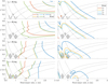 |
Fig. 1 Map of secular resonances in the (a, e0)-plane for a between 0.5 and 3 au, for different values of proper inclination, i0. The left column shows the locations of vj, j = 2,3,4,5,6, while the right column shows the locations of |

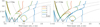 |
Fig. 2 Map of the vj, j = 2,3,4,5,6 secular resonances in the (a, e0)-plane for a between 0.5 and 3 au, at i0 = 5° (left panel), and at i0 = 2° (right panel). Dashed curves correspond to q = a2, a3, a4 and Q = a2, a3, a4 We also reported the location of the Kozai librators in grey, identified by ɡ − s = 0. |
3.2 Secular resonance maps at fixed eccentricity
We discretized the (a, i0)-plane with a step of 0.01 au for the semi-major axis, and 0.5° for the inclination. We took into account the region defined by 0.5 au < a < 3 au and 0° < i0 < 50°. The proper eccentricity was fixed, and we computed the maps for values e0 = 0.1 · h, h = 1,…,7, and for low eccentricity e0 = 0.02, 0.05. The left column of Fig. 3 shows the location of the vj,j = 2,…,6 secular resonances, while the right column shows the location of  , j = 2, 3, 4, 6, for values of proper eccentricity, e0, equal to 0.1, 0.2, 0.4, and 0.6. We note that the first row of Fig. 3 is the same case considered by Michel & Froeschlé (1997). The results we obtained are in really good agreement with those presented by Michel & Froeschlé (1997) (see Fig. 2 and 3 therein), with the difference that we are able to extend the maps to the planet-crossing regions. Figure 4 shows the same maps obtained for e0 = 0.05, 0.02.
From the left column of Fig. 3, we can see that all the resonances vj, j = 2,…, 6 appear in the region of 0.5 au < a < 3 au. As expected, V3 and V4 are always close to each other. At a proper eccentricity of e0 = 0.1, the v3, v4, and v6 resonances all have four different branches, each one appearing in the regions a > a4, a3 < a < a4, a2 < a < a3, and in a < a2. The v6 resonance with Saturn is confined at inclination smaller than about 20°. The resonances v2 and v5 have three different branches, each one appearing for a > a3, a2 < a < a3, and in a < a2. We can also notice the presence of Kozai librators around a = a2 and a = a3, which fill this area of the phase space up to i ≈ 35°.
At a proper eccentricity e0 = 0.2, the branches in the region a2 < a < a3 have almost disappeared, while those that were appearing at a < a2 are shifted to smaller values of semi-major axis, if compared with the previous case. For a > a3, the map is qualitatively similar to the case e0 = 0.1. The Kozai librators still appear near a2 and a3, but they fill a smaller area of the phase space, which is also moved towards larger inclinations. Moreover, another region filled by Kozai librators appears between Venus and the Earth, that corresponds to that seen in Fig. 1 for a proper inclination of 30°, and 40°. We found that the location of the secular resonances for e0 = 0.3 is qualitatively similar to e0 = 0.2 overall and, therefore, it is not shown.
The maps for e0 = 0.4 and e0 = 0.6 are also qualitatively similar to each other. The region at a ≲ 1.3 au is almost cleared out from all the secular resonances, which appear to a large extent at larger semi-major axis values, where they only have one branch. Moreover, they cover a larger interval of inclination values than in the previous cases. It is also worth noting that Kozai librators have disappeared, which is consistent with the results presented in Figs. 1 and 2.
The left column of Fig. 4 shows the maps obtained for e0 = 0.05 and 0.02. We can see they are qualitatively similar to what we obtained for e0 = 0.1. We can see that the Kozai resonance region is smaller than for the case e0 = 0.1, and the secular resonances extend closer to the semi-major axes of Venus, of the Earth, and of Mars.
The right column of Fig. 3 shows the location of the  , j= 2, 3, 4, 6 secular resonances. As seen in Sect. 3.1, the resonance ν12 with Venus is negligible. At an eccentricity of e0 = 0.1, we can see that ν16 has three different branches, while v13 and ν14 have only one. These three resonances are confined at semimajor axis smaller than 2.3 au and they span a large interval of inclination values. We note that ν13, ν14, and ν16 appear also in the Kozai resonance region. For a higher value of proper eccentricity, we can see that ν16 also have a single branch. Moreover, as e0 increases, their location moves towards smaller values of the semi-major axis and they span a smaller interval of inclinations. Finally, the right column of Fig. 4 shows the location of the
  resonances for e0 = 0.02 and 0.05. The maps are qualitatively similar to the case e0 = 0.1, with the difference that the three resonances involving the Earth, Mars, and Saturn all extend towards larger semi-major axis values.
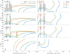 |
Fig. 3 Map of secular resonances in the (a, i0)-plane for a between 0.5 and 3 au, for different values of proper eccentricity, e0. The left column shows the locations of vj, j = 2, 3, 4, 5, 6, while the right column shows the locations of |

3.3 Frequencies near perihelion equal to planets' semi-major axes
Figures 1 and 2 show that the secular resonances tend to follow the perihelion curves a(1 − e) = aj, j = 2, 3, 4, and the trend is more prominent when the proper inclination, i0, decreases toward 0. To better understand the reason behind this effect, we computed the proper frequencies on a grid in eccentricity by fixing both the values of the semi-major axis and of the proper inclination. To gain a better picture of the behavior of the frequency, we also used a step in eccentricity of 5 × 10⁻⁴, which is smaller than that used to produce Figs. 1 and 2. Figure 5 shows the frequency ɡ computed for a = 1.2 au and i0 = 2°, as a function of the proper eccentricity, e0. When e0 approaches the critical values  , j = 2, 3 for which
  , the frequency ɡ sharply increases. Moreover, the magnitude of the increase is larger and larger as the inclination tends to 0°. This feature is caused by the model itself, and it is due to the orbit-crossing singularity.
Figure 5 shows also an interesting feature: between  and
and  , the frequency, ɡ, has a minimum that is smaller than ɡ5, which is the smallest planetary frequency. As e0 tends to
  from the right, the frequency, ɡ, increases sharply, and it crosses all the planetary frequencies ɡj, j = 2,…, 6 within a small interval of proper eccentricities, e0. The same happens as e0 tends to
  from the right, with the difference that only ɡ2 and ɡ5 are attained near the critical value. This effect causes the secular resonances to follow the Earth perihelion curve and to be close to each other. In addition, the fact that ɡ grows so fast in such a small interval of eccentricity will make the resonance width very small, so that objects following the perihelion curves by effect of the secular resonances will be extremely rare to find, because they would be pushed outside of the resonance by other small perturbations. In fact, we did not find any object following a planet's perihelion curve in our purely numerical integrations (see Sect. 3.4).
The sharp increase of the frequency ɡ near planets' perihelion curves also causes some small numerical errors in the global plot of the maps presented in Figs. 1 and 2. Because we use a discrete grid in the (a, e0)-plane, it may happen that a value larger than one of the planets' frequency, ɡj, is not achieved in the neighborhood of one of such perihelion curves. As a consequence, the corresponding secular frequency vj would not appear in the plot. This can be seen, for instance, in the maps at i0 = 2°, presented in Fig. 2. Figure 5 shows that all the five resonances vj, j = 2,…, 6 are crossed in a neighborhood of a = 1.2 au and e0 ≈ 0.17, while it is not clear that this would happen in the left panel shown in Fig. 2. This is caused by the fact that the grid is not dense enough in this tiny neighborhood. So, to prove this assumption, we recomputed the secular frequencies in the portion (a, e0) ∈ [1.15 au, 1.3 au] × [0.1, 0.3], using a step of 0.004 au in semi-major axis and of 5 × 10⁻⁴ in proper eccentricity. Figure 6 shows the location of the secular resonances in this portion of the phase space. Here, we can see that all the five secular resonances, vj, appear close to q = a3, even though v3,,v4, and v6 are barely distinguishable since they are very close to each other. Overall, we found these numerical effects to happen at low proper inclination, i0, and only near q = aj, j = 2, 3, 4, where the width of the resonance is very small in any case. Therefore, using a denser grid would not change the global picture of the secular resonances shown in Sect. 3.1, which was obtained using a less dense grid.
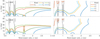 |
Fig. 4 Map of secular resonances in the (a, i0)-plane for a between 0.5 and 3 au, for different values of proper eccentricity, e0. The left column shows the locations of vj, j = 2, 3, 4, 5, 6, while the right column shows the locations of |

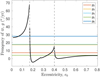 |
Fig. 5 Frequency, ɡ, (black solid curve) computed on a grid in proper eccentricity, e0, for a fixed value of semi-major axis of a = 1.2 au and proper inclination of i0 = 2°. The horizontal straight lines correspond to the values ɡj, j = 2, 3, 4, 5 of the proper frequencies of the planets. The vertical dashed lines correspond to the values of eccentricity, such that a(1 − e0) = aj, j = 2, 3. |
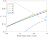 |
Fig. 6 Zoom on the map of the secular resonances vj, j = 2, 3, 4, 5, 6 at i0 = 2°, near a = 1.2au and e0 = 0.17. |
3.4 Comparison with numerical integrations
We performed purely numerical integrations to confirm the secular resonance locations predicted by the theory in Sects. 3.1 and 3.2. To account for the fact that the maps were computed in the proper elements space, we took initial orbital elements along the curves ɡ = ɡj (or S = Sj) and ɡ = ɡj ± 1" yr−1 (or S = Sj ± 1" yr−1), for a selected planet j ∈ {2, 3, 4, 5, 6}. The initial argument of pericenter, ω, and the initial argument of the node, Ω, were both set to 0°, while the initial mean anomaly, ℓ, was chosen randomly between 0° and 360°. Numerical integrations were performed by using a hybrid symplectic scheme (Chambers 1999) that is able to handle close encounters with planets, that is included in the MERCURY2 package (see also Fenucci & Novakovic 2022). The gravitational attraction of the Sun and of all the planets from Mercury to Neptune were included in the model and the initial conditions for planets at epoch 58800 MJD were taken from the JPL Horizons3 ephemeris system. We note that here we take into account a complete model of the Solar System to show that the simplified model presented in Sect. 2 is actually able to predict the location of secular resonances in a qualitative picture. We propagated the evolution of the asteroids and the planets for a total time of 2 Myr by using a timestep of one day.
We present here the results obtained by choosing an initial inclination of 20°. Figure 7 shows the evolution of a test asteroid selected with the method described above, which is affected by the ν6 secular resonance. The critical angle, ϖ − ϖS librates around 0°, while the eccentricity decreases down to values of about 0.4 during the first 0.2 Myr of evolution, and then suddenly increases up to values close to 1, causing this object to impact with the Sun in less than 0.5 Myr of dynamical evolution. This is a well-known effect of the ν6 resonance, found for the first time by Farinella et al. (1994), which is able to deliver Sun impactors even starting from the main belt at a very low eccentricity. This simulation shows that, as expected, this behavior still occurs well inside the NEO region, even at higher values of the initial eccentricity.
Figure 8 shows a test asteroid affected by the ν5 secular resonance. The critical angle ϖ − ϖJ librates around 0° during the 2 Myr of evolution and the eccentricity passes from an initial value of about 0.2 to values close to 0.6. The semi-major axis assumes values between 1.2 and 1.5 au, and it undergoes a random walk evolution, caused by close encounters with the inner planets. Despite the changes in the semi-major axis, the critical angle still librates and it is not removed from the secular resonance. Although this object did not end the evolution on a collision with the Sun, ν5 was able to push it to large eccentricity values, showing a behavior similar to that of ν6. By using numerical simulations, Gladman et al. (2000) showed that a combination of planetary close encounters and the ν5 secular resonance is a route to Sun-grazing orbits at semi-major axis a < 2 au. Therefore, ν5 could provide another significant mechanism for the delivery of asteroids impacting the Sun and the inner planets that acts well within the NEO region.
Figure 9 shows two test asteroids located near ν2 and ν3. These objects both show the corresponding critical argument librating around 0° but, in contrast to the previous examples, these resonances do not increase the eccentricity in the 2 My integration time-span. On the other hand, the test asteroid affected by ν3 shows an initial increasing of the inclination up to 30° caused by the effect of the resonance.
Here, we present only few examples corresponding to one of the maps of Fig. 1, however, all the numerical results obtained are in agreement with the locations computed for i0 = 20°. Therefore, we think that the maps obtained in Sects. 3.1 and 3.2 provide a reasonable estimation for the location of the secular resonances in the NEO region.
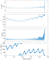 |
Fig. 7 Evolution of a test particle inside the ν6 secular resonance. The first three panels show the evolution of semi-major axis, eccentricity, and inclination, while the last panel shows the evolution of the critical angle ϖ − ϖS. |
4 Discussion
4.1 Possible dynamical paths inside the NEO region
Farinella et al. (1994) showed that the ν6 secular resonance is very efficient in increasing the eccentricity of asteroids initially located in the main belt, causing e to pass from values near to 0 to values near to 1 in just ~0.5 Myr. Foschini et al. (2000), Gladman et al. (2000) showed some numerical example in which the ν5 secular resonance increases the eccentricity of NEOs located at a < 2 au, causing asteroids to end up in a collision with the Sun. However, the location of the ν5 resonance inside the NEO region was not determined. In Sect. 3.4, we also showed an example where ν5 is able to pump up the eccentricity to values near to 1. Thus, some secular resonances are responsible for the delivery of asteroids impacting the planets or the Sun, even well inside the NEO region.
To search for possible dynamical paths, we took the population of known NEOs and identified those that are near the secular resonances. The nominal orbital elements were downloaded from the Near-Earth Objects Coordination Centre4 (NEOCC) on August 24, 2022. Then, we computed their proper frequencies ɡ, s, and their proper elements e0, i0, as we defined in Sect. 2. We plotted all the NEOs in the (a, e0) and in the (a, i0) planes and highlighted the objects near the vj, j = 2, 3, 5, 6 and v16 secular resonances, as well as Kozai librators. NEOs near v4 were not plotted because they almost overlap with v3. Since we did not attempt to compute the width of the resonances, we set an arbitrary threshold of 1" yr−1 for the identification of resonant objects that we believe to be a reasonable choice (see also Gronchi & Milani 2001). Figure 10 shows the result of the plot. We note that secular resonances appear as a swarm of points in this figure, differently to what described in Sect. 3. This is because here we show the projections of the whole three-dimensional space of the proper elements on a two-dimensional plane, and also because we assumed a non-zero resonance width. From the plot in the (a, e0)-plane, we can notice that objects near to v6 cross the curve q = a3, confirming again that this resonance is able to move objects onto Earth-crossing orbits (Bottke et al. 2002; Granvik et al. 2018). Moreover, NEOs near νj,·j = 2,…,6 extend to high eccentricity values, even surpassing 0.8. The fact that known NEOs are currently near these resonances and are placed at high eccentricity is an indication that all the vj resonances may be able to pump up the eccentricity and deliver objects impacting the Sun. It is worth also noting that there are NEOs near v16 between 1.5 au and 2 au that extend from the border of the NEO region at q = 1.3 au to q = a3. Therefore, this resonance might also be able to move asteroids onto Earth-crossing orbits. We note that v16 is near to the Hungaria region (see e.g. Froeschle & Scholl 1986), that is now recognized to be an important source region of NEOs (Granvik et al. 2018) producing a non-negligible fraction of Earth impactors.
Wetherill (1988) suggested that the v16 secular resonance could be responsible for the production of NEOs with inclinations larger than 30°. Later, Gladman et al. (2000) showed with numerical simulations that this mechanism is actually possible. In the right panel of Fig. 10, we can see objects at high inclinations near v2, v5, and v16, suggesting that they all could be capable of increasing the inclination. Indeed, the maps of Fig. 3 show that v2 and v5 extend towards values of the inclination larger than 50° for proper eccentricity of 0.6. Additionally, v12, v13, and v16 all extend towards high inclination values, regardless of the value of the proper eccentricity. Therefore, even if not reported in Fig. 10, also v12 and v13 could be responsible for increasing the inclination to values higher than 30°.
In this work, we only gave an indication of possible dynamical paths inside the NEO region that are based on the secular motion and on the current position of known NEOs. Additional extensive numerical simulations with a full N-body model need to be performed to better investigate and establish these hypotheses.
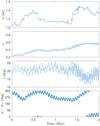 |
Fig. 8 Evolution of a test particle inside the v5 secular resonance. The last panel shows the evolution of the critical argument, ϖ − ϖ. |
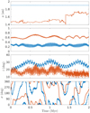 |
Fig. 9 Evolution of a test particle in the v2 (red curve), and another one in the v3 (blue curve) secular resonances. The last panel shows the evolution of the corresponding critical argument σ: ϖ − ϖV (red curve) for v2, and ϖ − ϖE (blue curve) for v3. |
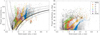 |
Fig. 10 Known NEOs close to some secular resonances, in the phase space (a,e0) (left panel) and (a, i0) (right panel). Gray dots represent the background population of NEOs, while red, yellow, green, blue, and violet correspond to the v2, v3, v5, v6 and v16, respectively. Black dots denote objects in the Kozai resonance. |
4.2 Effects of mean-motion resonances
The interaction between secular resonances and mean-motion resonances (MMRs) with Jupiter has been studied by Morbidelli & Moons (1993), Moons & Morbidelli (1995) in the main belt. The results presented in this paper were obtained with a semi-analytical model that does not take into account the effect of MMRs between the asteroid and a planet. One method for the computation of proper elements and frequencies of resonant NEOs, which extends that of Gronchi & Milani (2001), was recently developed by Fenucci et al. (2022). These authors showed that the secular evolution of asteroids that are placed well inside the strongest MMRs with Jupiter is significantly different from the non-resonant secular evolution, and that the frequencies, ɡ and s, are generally affected by these resonances. The same happens for some MMRs with the Earth, and Venus. On the contrary, MMRs with Mars have generally little effect on the long-term dynamics.
Some of the strongest MMRs with Jupiter, such as the 5:2, 7:3, and 2:1, are located beyond 2.5 au. The 3:1 MMR, that is the strongest one with Jupiter, is located at about 2.5 au. Therefore, they should not modify the results obtained for the nodal resonances  , since they always appear at a < 2.5 au, while they may somewhat affect the location of v3, v4, and v6 at inclinations, i0, larger than about 20°. On the other hand, the 7:2, 4:1, and 5:1 MMRs with Jupiter occur at smaller semi-major axis values, that is, at about 2.25 au, 2.06 au, and 1.78 au, respectively. Additionally, low-order resonances with Venus and the Earth mostly appear at a < 2.5 au (see e.g., Gallardo 2006), hence, they could all somewhat affect the secular resonances location.
Recently, Zhou et al. (2019), Xu et al. (2022) determined maps of secular resonances near the 1:1 MMR with the Earth and with Venus, computing the proper frequencies by using pure numerical integrations and frequency analysis (Laskar 1988, 1990, 2005). The maps obtained in these works do show some differences with respect to those presented in this paper. However, the effects of MMRs is only local and the secular resonances are affected only in a strip in semi-major axis of ~0.02 au width for the 1:1 MMR with the Earth and of ~0.008 au width for the 1:1 MMR with Venus.
To give a bigger picture of the strongest MMRs appearing at a < 2.5 au, we show their widths in Fig. 11. The width was computed with a simplified analytical method taken from Morbidelli (2002), for a fixed value of inclination of 15°. MMRs generally occupy a small volume of this part of the phase space and those with Venus and the Earth are especially narrow. This observation, coupled with the fact that MMRs significantly change the secular dynamics only when the asteroid is well inside the resonance (Fenucci et al. 2022), should limit the effect of MMRs on the results presented in this paper, that are aimed to give the general picture of the whole NEO region.
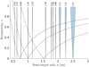 |
Fig. 11 Strongest mean-motion resonances at semi-major axis a < 2.5 au. The filled light-blue area represents the resonance width, computed with an analytic method (see Morbidelli 2002) for a fixed value of inclination of 15°. |
5 Conclusions
In this paper, we determined the location of the secular resonances with the planets from Venus to Neptune inside the NEO region. Proper elements and proper frequencies of NEOs were computed by using a semi-analytical secular model that allow for the propagation of the secular evolution of objects beyond orbit-crossing singularities. Maps of the secular resonances were then obtained by keeping the proper inclination, i0, (or the proper eccentricity, e0) at a fixed value, and we showed how the locations change by varying the value of the fixed proper element.
The vj, j = 2,…,6 secular resonances all appear well inside the NEO region, especially at inclinations smaller than about 30°. On the other hand, the  secular resonances with the node of the planets mainly appear solely for j = 3, 4, 6, and they tend to be negligible at small inclinations. To confirm the computed locations, we performed full numerical N-body simulations that included all the planets of the Solar System. The results obtained showed that the maps computed with the semi-analytical approach provide a good estimate of the secular resonance locations. The current distribution of NEOs close to secular resonances suggests that some of these resonances could be able to produce Sun-grazing asteroids and Earth impactors -or they may increase the inclination to values bigger than 30°.
Acknowledgements
The authors have been supported by the MSCA-ITN Stardust-R, Grant Agreement no. 813644 under the European Union H2020 research and innovation program. GFG also acknowledges the project MIUR-PRIN 20178CJA2B "New frontiers of Celestial Mechanics: theory and applications" and the GNFM-INdAM (Gruppo Nazionale per la Fisica Matematica).
References
- Bottke, W.F., Morbidelli, A., Jedicke, R., et al. 2002, Icarus, 156, 399 [NASA ADS] [CrossRef] [Google Scholar]
- Chambers, J.E. 1999, MNRAS, 304, 793 [NASA ADS] [CrossRef] [Google Scholar]
- Farinella, P., Froeschle, C., Froeschle, C., et al. 1994, Nature, 371, 315 [Google Scholar]
- Fenucci, M., & Novakovic, B. 2022, Serb. Astron. J., 204, 51 [NASA ADS] [CrossRef] [Google Scholar]
- Fenucci, M., Gronchi, G.F., & Saillenfest, M. 2022, Celest. Mech. Dyn. Astron., 134, 23 [NASA ADS] [CrossRef] [Google Scholar]
- Foschini, L., Farinella, P., Froeschlé, C., et al. 2000, A&A, 353, 797 [NASA ADS] [Google Scholar]
- Froeschle, C., & Scholl, H. 1986, A&A, 166, 326 [NASA ADS] [Google Scholar]
- Froeschle, C., & Scholl, H. 1989, Celest. Mech. Dyn. Astron., 46, 231 [NASA ADS] [CrossRef] [Google Scholar]
- Gallardo, T. 2006, Icarus, 184, 29 [Google Scholar]
- Gallardo, T., Hugo, G., & Pais, P. 2012, Icarus, 220, 392 [NASA ADS] [CrossRef] [Google Scholar]
- Gladman, B., Michel, P., & Froeschlé, C. 2000, Icarus, 146, 176 [NASA ADS] [CrossRef] [Google Scholar]
- Granvik, M., Morbidelli, A., Vokrouhlickÿ, D., et al. 2017, A&A, 598, A52 [NASA ADS] [CrossRef] [EDP Sciences] [Google Scholar]
- Granvik, M., Morbidelli, A., Jedicke, R., et al. 2018, Icarus, 312, 181 [CrossRef] [Google Scholar]
- Gronchi, G.F., & Milani, A. 1998, Celest. Mech. Dyn. Astron., 71, 109 [NASA ADS] [CrossRef] [Google Scholar]
- Gronchi, G.F., & Milani, A. 2001, Icarus, 152, 58 [NASA ADS] [CrossRef] [Google Scholar]
- Gronchi, G.F., & Tardioli, C. 2013, Discrete Continuous Dyn. Syst. B, 18, 1323 [CrossRef] [Google Scholar]
- Knezevic, Z. 2020, MNRAS, 497, 4921 [NASA ADS] [CrossRef] [Google Scholar]
- Knezevic, Z. 2022, Serb. Astron. J., 204, 1 [NASA ADS] [CrossRef] [Google Scholar]
- Knezevic, Z., & Milani, A. 2000, Celest. Mech. Dyn. Astron., 78, 17 [NASA ADS] [CrossRef] [Google Scholar]
- Knezevic, Z., & Milani, A. 2003, A&A, 403, 1165 [NASA ADS] [CrossRef] [EDP Sciences] [Google Scholar]
- Knezevic, Z., & Milani, A. 2019, Celest. Mech. Dyn. Astron., 131, 27 [NASA ADS] [CrossRef] [Google Scholar]
- Knezevic, Z., Milani, A., Farinella, P., Froeschle, C., & Froeschle, C. 1991, Icarus, 93, 316 [NASA ADS] [CrossRef] [Google Scholar]
- Kozai, Y. 1962, AJ, 67, 591 [Google Scholar]
- Laskar, J. 1988, A&A, 198, 341 [NASA ADS] [Google Scholar]
- Laskar, J. 1990, Icarus, 88, 266 [NASA ADS] [CrossRef] [Google Scholar]
- Laskar, J. 2005, Frequency Map Analysis and Quasiperiodic Decompositions (Cambridge Scientific Pub.), 99 [Google Scholar]
- Laskar, J., Robutel, P., Joutel, F., et al. 2004, A&A, 428, 261 [NASA ADS] [CrossRef] [EDP Sciences] [Google Scholar]
- Laskar, J., Fienga, A., Gastineau, M., & Manche, H. 2011, A&A, 532, A89 [NASA ADS] [CrossRef] [EDP Sciences] [Google Scholar]
- Michel, P., & Froeschlé, C. 1997, Icarus, 128, 230 [NASA ADS] [CrossRef] [Google Scholar]
- Milani, A., & Knezevic, Z. 1990, Celest. Mech. Dyn. Astron., 49, 347 [NASA ADS] [CrossRef] [Google Scholar]
- Milani, A., & Knezevic, Z. 1994, Icarus, 107, 219 [NASA ADS] [CrossRef] [Google Scholar]
- Moons, M., & Morbidelli, A. 1995, Icarus, 114, 33 [NASA ADS] [CrossRef] [Google Scholar]
- Morbidelli, A. 2002, Modern Celestial Mechanics: Aspects of Solar System Dynamics (Taylor and Francis) [Google Scholar]
- Morbidelli, A., & Henrard, J. 1991a, Celest. Mech. Dyn. Astron., 51, 131 [NASA ADS] [CrossRef] [Google Scholar]
- Morbidelli, A., & Henrard, J. 1991b, Celest. Mech. Dyn. Astron., 51, 169 [NASA ADS] [CrossRef] [Google Scholar]
- Morbidelli, A., & Moons, M. 1993, Icarus, 102, 316 [NASA ADS] [CrossRef] [Google Scholar]
- Nobili, A.M., Milani, A., & Carpino, M. 1989, A&A, 210, 313 [NASA ADS] [Google Scholar]
- Saillenfest, M., Fouchard, M., Tommei, G., & Valsecchi, G.B. 2016, Celest. Mech. Dyn. Astron., 126, 369 [NASA ADS] [CrossRef] [Google Scholar]
- Scholl, H. & Froeschle, C. 1986, A&A, 170, 138 [NASA ADS] [Google Scholar]
- Thomas, F., & Morbidelli, A. 1996, Celest. Mech. Dyn. Astron., 64, 209 [NASA ADS] [CrossRef] [Google Scholar]
- Tsirvoulis, G., & Novakovic, B. 2016, Icarus, 280, 300 [NASA ADS] [CrossRef] [Google Scholar]
- Wetherill, G.W. 1988, Icarus, 76, 1 [NASA ADS] [CrossRef] [Google Scholar]
- Williams, J.G. 1969, PhD thesis, University Of California, Los Angeles, USA [Google Scholar]
- Williams, J.G., & Faulkner, J. 1981, Icarus, 46, 390 [NASA ADS] [CrossRef] [Google Scholar]
- Xu, Y.-B., Zhou, L., Lhotka, C., Zhou, L.-Y., & Ip, W.-H. 2022, A&A, 666, A88 [NASA ADS] [CrossRef] [EDP Sciences] [Google Scholar]
- Yoshikawa, M. 1987, Celest. Mech., 40, 233 [NASA ADS] [CrossRef] [Google Scholar]
- Zhou, L., Xu, Y.-B., Zhou, L.-Y., Dvorak, R., & Li, J. 2019, A&A, 622, A97 [NASA ADS] [CrossRef] [EDP Sciences] [Google Scholar]
The symbol ɡ is also used to denote the secular frequency of the longitude of perihelion ϖ, as mentioned in the introduction. However, it is clear from the context when we use ɡ to refer to the argument of the pericenter, ω, or to refer to the frequency of ϖ.
All Tables
Secular frequencies of the planets from Venus to Saturn, as determined by Laskar et al. (2011).
All Figures
|
Fig. 1 Map of secular resonances in the (a, e0)-plane for a between 0.5 and 3 au, for different values of proper inclination, i0. The left column shows the locations of vj, j = 2,3,4,5,6, while the right column shows the locations of |
| In the text | |
|
Fig. 2 Map of the vj, j = 2,3,4,5,6 secular resonances in the (a, e0)-plane for a between 0.5 and 3 au, at i0 = 5° (left panel), and at i0 = 2° (right panel). Dashed curves correspond to q = a2, a3, a4 and Q = a2, a3, a4 We also reported the location of the Kozai librators in grey, identified by ɡ − s = 0. |
| In the text | |
|
Fig. 3 Map of secular resonances in the (a, i0)-plane for a between 0.5 and 3 au, for different values of proper eccentricity, e0. The left column shows the locations of vj, j = 2, 3, 4, 5, 6, while the right column shows the locations of |
| In the text | |
|
Fig. 4 Map of secular resonances in the (a, i0)-plane for a between 0.5 and 3 au, for different values of proper eccentricity, e0. The left column shows the locations of vj, j = 2, 3, 4, 5, 6, while the right column shows the locations of |
| In the text | |
|
Fig. 5 Frequency, ɡ, (black solid curve) computed on a grid in proper eccentricity, e0, for a fixed value of semi-major axis of a = 1.2 au and proper inclination of i0 = 2°. The horizontal straight lines correspond to the values ɡj, j = 2, 3, 4, 5 of the proper frequencies of the planets. The vertical dashed lines correspond to the values of eccentricity, such that a(1 − e0) = aj, j = 2, 3. |
| In the text | |
|
Fig. 6 Zoom on the map of the secular resonances vj, j = 2, 3, 4, 5, 6 at i0 = 2°, near a = 1.2au and e0 = 0.17. |
| In the text | |
|
Fig. 7 Evolution of a test particle inside the ν6 secular resonance. The first three panels show the evolution of semi-major axis, eccentricity, and inclination, while the last panel shows the evolution of the critical angle ϖ − ϖS. |
| In the text | |
|
Fig. 8 Evolution of a test particle inside the v5 secular resonance. The last panel shows the evolution of the critical argument, ϖ − ϖ. |
| In the text | |
|
Fig. 9 Evolution of a test particle in the v2 (red curve), and another one in the v3 (blue curve) secular resonances. The last panel shows the evolution of the corresponding critical argument σ: ϖ − ϖV (red curve) for v2, and ϖ − ϖE (blue curve) for v3. |
| In the text | |
|
Fig. 10 Known NEOs close to some secular resonances, in the phase space (a,e0) (left panel) and (a, i0) (right panel). Gray dots represent the background population of NEOs, while red, yellow, green, blue, and violet correspond to the v2, v3, v5, v6 and v16, respectively. Black dots denote objects in the Kozai resonance. |
| In the text | |
|
Fig. 11 Strongest mean-motion resonances at semi-major axis a < 2.5 au. The filled light-blue area represents the resonance width, computed with an analytic method (see Morbidelli 2002) for a fixed value of inclination of 15°. |
| In the text | |
Current usage metrics show cumulative count of Article Views (full-text article views including HTML views, PDF and ePub downloads, according to the available data) and Abstracts Views on Vision4Press platform.
Data correspond to usage on the plateform after 2015. The current usage metrics is available 48-96 hours after online publication and is updated daily on week days.
Initial download of the metrics may take a while.