| Issue |
A&A
Volume 666, October 2022
|
|
|---|---|---|
| Article Number | A46 | |
| Number of page(s) | 17 | |
| Section | Planets and planetary systems | |
| DOI | https://doi.org/10.1051/0004-6361/202243583 | |
| Published online | 04 October 2022 | |
Two long-period transiting exoplanets on eccentric orbits: NGTS-20 b (TOI-5152 b) and TOI-5153 b★
1
Observatoire de Genève, Université de Genève,
Chemin Pegasi, 51,
1290
Versoix, Switzerland
e-mail: This email address is being protected from spambots. You need JavaScript enabled to view it.
2
Department of Physics, University of Warwick,
Gibbet Hill Road,
Coventry
CV4 7AL, UK
3
Centre for Exoplanets and Habitability, University of Warwick,
Gibbet Hill Road,
Coventry
CV4 7AL, UK
4
Department of Physics and Kavli Institute for Astrophysics and Space Research, Massachusetts Institute of Technology,
Cambridge, MA
02139, USA
5
Max-Planck-Institut für Astronomie,
Königstuhl 17,
69117
Heidelberg, Germany
6
Facultad de Ingeniería y Ciencias, Universidad Adolfo Ibáñez,
Av. Diagonal las Torres
2640,
Peñalolén, Santiago, Chile
7
Millennium Institute for Astrophysics,
Chile
8
Department of Physics and Astronomy, University of New Mexico,
1919 Lomas Blvd NE
Albuquerque, NM
87131, USA
9
Physikalisches Institut, University of Bern,
Gesellschaftsstrasse 6,
3012
Bern, Switzerland
10
School of Physics and Astronomy, University of Leicester,
Leicester
LE1 7RH, UK
11
Center for Astrophysics, Harvard & Smithsonian,
60 Garden Street,
Cambridge, MA
02138, USA
12
Institute of Planetary Research, German Aerospace Center,
Ruther-fordstrasse 2,
12489
Berlin, Germany
13
Fisk University,
Nashville, TN, USA
14
Vanderbilt University,
Nashville, TN, USA
15
Department of Astronomy, Ohio State University,
140 W. 18th Ave.,
Columbus, OH
43210, USA
16
Astronomy Unit, Queen Mary University of London,
Mile End Road,
London
E1 4NS, UK
17
Astrophysics Group, Cavendish Laboratory,
J.J. Thomson Avenue,
Cambridge
CB3 0HE, UK
18
Department of Astronomy & Astrophysics, 525 Davey Laboratory, The Pennsylvania State University,
University Park, PA
16802, USA
19
Center for Exoplanets and Habitable Worlds, 525 Davey Laboratory, The Pennsylvania State University,
University Park, PA
16802, USA
20
European Space Agency (ESA), European Space Research and Technology Centre (ESTEC),
Keplerlaan 1,
2201 AZ
Noordwijk, The Netherlands
21
Núcleo de Astronomía, Facultad de Ingeniería y Ciencias, Universidad Diego Portales,
Av. Ejército 441,
Santiago, Chile
22
Centro de Astrofísica y Tecnologías Afines (CATA),
Casilla 36-D,
Santiago, Chile
23
European Southern Observatory,
Alonso de Córdova 3107, Vitacura, Casilla
19001,
Santiago, Chile
24
Department of Physics and Astronomy, University of New Mexico,
210 Yale Blvd NE
Albuquerque, NM
87106, USA
25
Instituto de Astronomía, Universidad Católica del Norte,
Angamos 0610,
1270709,
Antofagasta, Chile
26
Center for Space and Habitability, University of Bern,
Gesellschaftsstrasse 6,
3012,
Bern, Switzerland
27
Department of Physics, Lehigh University,
16 Memorial Drive East,
Bethlehem, PA
18015, USA
28
ETH Zurich, Department of Physics,
Wolfgang-Pauli-Strasse 27,
8093
Zurich, Switzerland
29
Center for Astrophysics, Harvard & Smithsonian,
60 Garden Street,
Cambridge, MA
02138, USA
30
Instituto de Astrofísica, Pontificia Universidad Católica de Chile,
Avda. Vicuña Mackenna
4860,
Macul, Santiago, Chile
31
Millennium Institute of Astrophysics,
Nuncio Monsenor Sotero Sanz 100, Of. 104,
Providencia, Santiago, Chile
32
Department of Astronomy/Steward Observatory, The University of Arizona,
933 North Cherry Avenue,
Tucson, AZ
85721, USA
33
Department of Astronomy, Sofia University “St Kliment Ohridski”,
5 James Bourchier Blvd,
BG-1164
Sofia, Bulgaria
34
Departamento de Astronomía, Universidad de Chile,
Casilla 36-D,
Santiago, Chile
35
Shanghai Astronomical Observatory, Chinese Academy of Sciences,
80 Nandan Road,
Shanghai
200030, PR China
36
Centre for Astrophysics, University of Southern Queensland,
West Street,
Toowoomba,
QLD 4350, Australia
Received:
18
March
2022
Accepted:
6
July
2022
Abstract
Context. Long-period transiting planets provide the opportunity to better understand the formation and evolution of planetary systems. Their atmospheric properties remain largely unaltered by tidal or radiative effects of the host star, and their orbital arrangement reflects a different and less extreme migrational history compared to close-in objects. The sample of long-period exoplanets with well-determined masses and radii is still limited, but a growing number of long-period objects reveal themselves in the Transiting Exoplanet Survey Satellite (TESS) data.
Aims. Our goal is to vet and confirm single-transit planet candidates detected in the TESS space-based photometric data through spectroscopic and photometric follow-up observations with ground-based instruments.
Methods. We used high-resolution spectrographs to confirm the planetary nature of the transiting candidates and measure their masses. We also used the Next Generation Transit Survey (NGTS) to photometrically monitor the candidates in order to observe additional transits. Using a joint modeling of the light curves and radial velocities, we computed the orbital parameters of the system and were able to precisely measure the mass and radius of the transiting planets.
Results. We report the discovery of two massive, warm Jupiter-size planets, one orbiting the F8-type star TOI-5153 and the other orbiting the G1-type star NGTS-20 (=TOI-5152). From our spectroscopic analysis, both stars are metal rich with a metallicity of 0.12 and 0.15, respectively. Only TOI-5153 presents a second transit in the TESS extended mission data, but NGTS observed NGTS-20 as part of its mono-transit follow-up program and detected two additional transits. Follow-up high-resolution spectroscopic observations were carried out with CORALIE, CHIRON, FEROS, and HARPS. TOI-5153 hosts a planet with a period of 20.33 days, a planetary mass of 3.26−0.17+0.18 Jupiter masses (MJ), a radius of 1.06−0.04+0.04 RJ, and an orbital eccentricity of 0.091−0.026+0.024. NGTS-20 b is a 2.98−0.15+0.16 MJ planet with a radius of 1.07−0.04+0.04 RJ on an eccentric 0.432−0.023+0.023 orbit with an orbital period of 54.19 days. Both planets are metal enriched and their heavy element content is in line with the previously reported mass-metallicity relation for gas giants.
Conclusions. Both warm Jupiters orbit moderately bright host stars, making these objects valuable targets for follow-up studies of the planetary atmosphere and measurement of the spin-orbit angle of the system.
Key words: planetary systems / planets and satellites: detection / planets and satellites: individual: NGTS 20/TOI-5152 / planets and satellites: individual: TOI-5153 / planets and satellites: gaseous planets / methods: data analysis
Full Tables 1 and 2 are only available at the CDS via anonymous ftp to cdsarc.u-strasbg.fr (130.79.128.5) or via http://cdsarc.u-strasbg.fr/viz-bin/cat/J/A+A/666/A46
Corresponding author: S. Ulmer-Moll, e-mail: This email address is being protected from spambots. You need JavaScript enabled to view it.
Winton Fellow.
ESA Research Fellow.
© S. Ulmer-Moll et al. 2022
 Open Access article, published by EDP Sciences, under the terms of the Creative Commons Attribution License (https://creativecommons.org/licenses/by/4.0), which permits unrestricted use, distribution, and reproduction in any medium, provided the original work is properly cited.
This article is published in open access under the Subscribe-to-Open model. This email address is being protected from spambots. You need JavaScript enabled to view it. to support open access publication.
1 Introduction
The majority of known transiting gas giants are hot Jupiters; they orbit their host star with periods of less than ten days. The extended atmospheres of hot Jupiters are ideal for atmospheric studies and for investigating their composition (e.g., Madhusudhan et al. 2014; Sing et al. 2016; Wyttenbach et al. 2017; Showman et al. 2020; Baxter et al. 2021), but the original properties of these systems are not often preserved (e.g., Albrecht et al. 2012). The orbital parameters of an exoplanet are the result of its origin and formation but in the case of close-in planets, such as hot Jupiters, the proximity of the host star leads to additional mechanisms such as tidal interactions (e.g., Valsecchi et al. 2015), which disturb the initial orbital parameters. Longer period transiting planets, such as warm Jupiters, are less affected by their host star and their orbital elements retain a record of their formation and migrational history.
Warm Jupiters are exoplanets orbiting their host star with periods typically defined between 10 and 200 days. Similarly to hot Jupiters, if warm Jupiters are not formed in situ, they require migration mechanisms that are able to bring them from several astronomical units (au) to a fraction of an au from their host star (Dawson & Johnson 2018). Part of the warm-Jupiter population is located in the period valley, a region of the parameter space between 10 and 100 days where gas giants are less frequent (Udry et al. 2003; Wittenmyer et al. 2010). The occurrence rates of gas giants can also suggest the type of formation and evolution undertaken by these objects. One of the distinctive features of the warm-Jupiter population is its wide range of eccentricities. The formation and evolution processes leading to the diversity of orbital arrangements seen in systems hosting warm Jupiters remain to be fully understood.
Several explanations have been put forward to explain the wide eccentricity distribution of warm Jupiters. The eccentricity distribution of warm Jupiters is composed of two groups, a low-eccentricity component and a higher eccentricity one (e.g., Petrovich & Tremaine 2016). Disk migration (e.g., Goldreich & Tremaine 1980; Baruteau et al. 2014) is able to explain the lower eccentricity component and can reproduce the period distribution of gas giants under certain disk properties (Coleman & Nelson 2016). However, disk migration and ensuing planet-planet scattering do not create enough warm Jupiters with high eccentricities (Petrovich et al. 2014). In high-eccentricity migration scenarios (e.g., Rasio & Ford 1996; Fabrycky & Tremaine 2007), warm Jupiters are the precursors of the hot Jupiters that we are observing in the midst of inward migration. High-eccentricity migration produces a satisfying number of warm Jupiters at high eccentricities but an insufficient number of low-eccentricity warm Jupiters. In addition, high-eccentricity migration under-produces warm Jupiters (Wu & Lithwick 2011), while disk migration produces a number of warm Jupiters that is coherent with the estimate of the period valley. Therefore, it is thought that a combination of these mechanisms could explain the observed population.
The composition of gas giants depends on where they are formed in the protoplanetary disk, on which timescales, but also on the composition of the disk. Measuring precise masses and radii of giant planets enables estimations of their bulk metallicity, which in turn constrains the formation and evolution models. Solar System giants are metal-enriched compared to the Sun (e.g., Wong et al. 2004) and core-accretion models are able to match their heavy metal enhancement (e.g., Alibert et al. 2005). For exoplanets, Thorngren et al. (2016) showed that the planet metal enrichment (Zplanet/Zstar) is anti-correlated with planetary mass, while the mass of heavy elements is positively correlated with planetary mass. Comparing the results of different planetary synthesis models with the bulk metallicity and atmospheric composition of exoplanets leads to constraints on the processes driving core formation and envelope enrichment (e.g., Mordasini et al. 2014, 2016). However, the sample of warm Jupiters with precise mass and radius measurements is scarce, and the correlation between planet metal-enrichment and planetary mass requires further investigation, for example in terms of detailed host star abundances (Teske et al. 2019) and in terms of its dependence on orbital properties of the planetary systems (Dalba et al. 2022).
Detecting transiting warm Jupiters is challenging, especially for ground-based surveys, as partial or full transit events visible from a given site are rare. However, the space-based photometric mission Transiting Exoplanet Survey Satellite (TeSS; Ricker et al. 2015) is opening up a new possibility to detect this type of exoplanet orbiting bright and well-characterized stars. TeSs observes each field almost continuously for 27 days, but a significant fraction of the sky is covered for longer periods of time when fields overlap. As such, TESS monitors some parts of the sky for up to one year in regions called continuous viewing zones. For fields observed continuously for 27 days, we expect most warm Jupiters to show only a single transit. Simulations by Cooke et al. (2018) and Villanueva et al. (2019) predicted that between 500 and 1000 single-transit events would be found in the first two years of the TESS data. Following these results, several pipelines have been developed to search for these events (e.g., Gill et al. 2020a; Montalto et al. 2020). These dedicated searches provide valuable candidates in addition to those announced by the TESS Objects of Interest (TOIs; Guerrero et al. 2021).
Single-transit candidates have several observational disadvantages; for example their orbital period is largely unconstrained. An estimate of the orbital period can be determined based on stellar and transit parameters (Osborn et al. 2016). With the re-observation of previous TESS sectors through the extended mission, new single-transit candidates are detected and several of the known candidates show a second transit, constraining the possible planetary periods to a discrete set of values. These candidates require spectroscopic vetting as we expect a false-positive rate of about 50% (Santerne et al. 2016). A byproduct of the search for warm Jupiters is therefore the detection and characterization of long-period low-mass eclipsing binaries (e.g., Lendl et al. 2020; Gill et al. 2022). Single and duo transit candidates are challenging systems to follow up and characterize but they can reveal warm planets, which are highly valuable systems (e.g., Osborn et al. 2022; Schanche et al. 2022). Long-period transiting giants are the missing link between hot Jupiters and the Solar System giants and they offer precious information for understanding the physics of their atmosphere, formation, migration, and their evolution history.
This paper describes the discovery and characterization of two new warm Jupiters. The observations are detailed in Sect. 2, the derivation of stellar parameters and the methods used to analyze photometric and radial velocity data are explained in Sect. 3. The results are presented in Sect. 4 and discussed in Sect. 5. We summarize our findings in Sect. 6.
2 Observations
The discovery photometry was collected with the space-based mission TESS (Sect. 2.1) and follow-up observations were carried out from the ground with the photometric facility NGTS (Sect. 2.2), and the high-resolution spectrographs CORALIE, FEROS, CHIRON, HARPS, and TRES (Sects. 2.3, 2.4, 2.5, 2.6, and 2.7). The presence of nearby stars was checked with speckle imaging (Sect. 2.8).
2.1 TESS photometry
TOI-5153 and NGTS-20 were observed by the TESS satellite during its primary and extended mission. Both targets showed a single-transit event, TOI-5153 in sector 4 and NGTS-20 in sector 6. As several teams set out to search for and vet this type of event, these stars were selected as single-transit candidates by the TSTPC (Tess Single Transit Planetary Candidate) group, and later announced as CTOIs (Community Tess Object of Interest) by J. Steuer and the WINE team. TOI-5153 was observed at a 30 min cadence in sector 6 (11 December 2018 to 7 January 2019) and at a two-minute cadence in sector 33 (17 December 2020 to 13 January 2021). NGTS-20 was observed at a 30 min cadence in sector 4 from 18 October 2018 to 15 November 2018 and at a two-minute cadence in sector 31 from 21 October 2020 to 19 November 2020. Both stars were observed at a two-minute cadence in the extended mission, thanks to the approved Guest Investigator Program G03188 led by S. Villanueva. However, only TOI-5153 showed a second single transit in sector 33 and no event was detected in sector 31 for NGTS-20. Both primary transits passed the vetting stage where we checked for asteroid crossing and centroid shifts (indicating a background eclipsing binary).
Light curves of the primary mission were extracted with the Quick Look Pipeline (QLP, Huang et al. 2020a,b). The light curves from the extended mission were obtained through the data reduction carried out at the Science Processing Operation Center (SPOC, Jenkins et al. 2016). We use the simple aperture photometry (SAP) fluxes and their corresponding errors for our analysis. The light curves are presented in Figs. 1 and 2. We generated target pixel files with tpf plotter (Aller et al. 2020) and checked for the presence of contaminant sources - down to a magnitude difference of 6 - within the aperture used to extract the light curves. One star (TIC 124029687) falls into the aperture around TOI-5153. We estimate the dilution by comparing the fluxes measured in the Gaia passband RP as this filter matches the TESS passband. TOI-5153 has a mean RP flux of 273878 ± 52 electrons per second (e−1 s−1) and TIC 124029687 has a flux of 2208 ± 8 e−1 s−1. The dilution is equal to 0.8 ± 0.003% (Eq. (6) from Espinoza et al. 2019). We included a dilution factor for the light curve modeling and chose a Normal prior informed by the dilution estimated with Gaia photometry. The aperture of NGTS-20 is not contaminated by neighboring stars, and therefore we chose to fix the dilution factor to 1 (no dilution) for the modeling of the light curve.
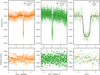 |
Fig. 1 Top: photometric observations of TOI-5153 from TESS sector 6 at 30 min cadence (orange dots, left panel) and sector 33 at 10 min cadence (green dots, middle panel) with full median models (orange and green lines), and Gaussian process models (black line). The right panel shows the detrended and phase-folded data from both sectors (orange and green dots) with the phase-folded transit model in black. Bottom: each panel shows the residuals in parts per million between the full model and the respective light curve. |
2.2 NGTS photometry
NGTS-20 was monitored from the ground by the Next Generation Transit Survey (NGTS). NGTS is an automated array of twelve 20 cm telescopes installed at ESO’s Paranal Observatory, Chile (Wheatley et al. 2018). NGTS uses a custom filter which spans 520–890 nm. Starting on the night of September 29, 2020, the target was observed in the blind survey mode (every possible night) with one 20 cm telescope. The data were acquired with an exposure time of 10 s and cadence of 13 s. Data reduction is performed with SAP and an automatic transit search is done using template matching (Gill et al. 2020b). One full transit was observed on the night of December 8, 2020. After this second transit event, the possible periods for this candidate correspond to a set of period aliases. The target was only observed on nights when a transit of a period alias was expected. A third transit was observed on the night of October 28,2021. Six NGTS cameras were used with the same exposure time and cadence as during the blind search survey mode. The NGTS light curves are presented in Fig. 2.
2.3 CORALIE spectroscopy
Spectroscopic vetting and radial velocity follow-up were carried out with the CORALIE spectrograph (Queloz et al. 2001). CORALIE is a fiber-fed spectrograph installed at the Nasmyth focus of the Swiss 1.2 m Euler telescope (La Silla, Chile). CORALIE has a spectral resolution of 60 000 and observes with a 3 pixel sampling per resolution element. Fiber injection is done with two fibers: a first fiber is used to observe the target and a second fiber can collect light from a Fabry-Pérot etalon or the sky to allow for simultaneous wavelength calibration or background subtraction.
TOI-5153 and NGTS-20 are part of an ongoing CORALIE survey that is designed to confirm TESS single-transit candidates and characterize the properties of the systems. Spectroscopic vetting is first done by taking two spectra of the target about one week apart. These two observations are used to rule out eclipsing binary scenarios. Each target is then monitored with an average of one point per week, and the sampling is adapted to maximize the phase coverage of the orbit once a periodic signal is detected.
Stellar radial velocities are measured with the cross-correlation technique: the stellar spectrum is cross-correlated with a mask close to the stellar type of the host star to obtain a cross-correlation function (CCF; e.g., Pepe et al. 2002). In addition to the radial velocity and its associated error, full width half maximum, contrast, and bisector inverse slope (BIS) are some of the parameters derived from the CCF. These parameters have been shown to be reliable tracers of the radial velocity noise induced by stellar activity and they can be used to detrend the data in some cases (e.g., Melo et al. 2007).
We collected 25 radial velocity measurements of TOI-5153 (from 9 December 2020 to 28 April 2021) and 39 measurements of NGTS-20 (from 17 November 2019 to 10 November 2021) with an exposure time varying between 900 and 1800s. The spectra of TOI-5153 have an average signal-to-noise ratio (S/ N) of 14 and those of NGTS-20 have an average S/N of 23. The observations for both targets are detailed in Tables 1 and 2 and are plotted in Figs. 3 and 4. CORALIE spectra were also used to derive stellar parameters and the analysis is detailed in Sect. 3.1.
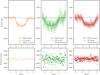 |
Fig. 2 Top: photometric observations of NGTS-20 from TESS sector 4 at 30 min cadence (left panel) and NGTS binned at two-minute cadence {middle and right panels). In each panel, the data are shown are colored dots (orange, green, and red), the full model is represented with a line of the same color, and the Gaussian process model is shown as a gray line. Bottom: each panel shows the residuals in parts per million between the full model and the respective light curve. |
Radial velocities of TOI-5153.
2.4 FEROS spectroscopy
FEROS is a high-resolution spectrograph installed at the 2.2 m telescope in La Silla, Chile. FEROS has a spectral resolution of 48 000 with 3 pixel sampling. Two fibers are available to observe the target and simultaneously record the spectrum of Th-Ar lamp to allow a precise wavelength calibration (Kaufer et al. 1999).
A total of nine FEROS spectra were collected for TOI-5153 between 20 February 2021 and 9 October 2021 under the program number 0106A-9014(A) (PI: Sarkis). The exposure times vary between 900 and 1200 s depending on the weather conditions. For NGTS-20,13 spectra were recorded under the program number 0104A-9007(A) (PI: Sarkis) between 25 February 2020 and 9 January 2021. Exposure times vary between 900 s and 1350 s depending on weather conditions and lead to a S/N ranging from 70 to 123.
The data reduction was performed with the CERES pipeline (Brahm et al. 2017), and the radial velocities were extracted using the cross-correlation technique. Radial velocity measurements are detailed in Tables 1 and 2 and plotted in Figs. 3 and 4.
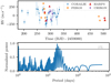 |
Fig. 3 Top: time series of the radial velocities from CORALIE (blue dots), FEROS (orange crosses), HARPS (red triangles), and CHIRON (purple stars) for TOI-5153. Bottom: generalized Lomb-Scargle periodogram of the radial velocities. The highest peak corresponds to a period of about 20.1 days. |
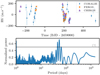 |
Fig. 4 Top: time series of the radial velocities from CORALIE (blue dots), FEROS (orange crosses), and CHIRON (purple triangles) for NGTS-20. Bottom: generalized Lomb-Scargle periodogram of the radial velocities. The highest peak corresponds to a period of about 53.5 days. |
Radial velocities of NGTS-20.
2.5 CHIRON spectroscopy
TOI-5153 was observed with the CHIRON spectrograph (Tokovinin et al. 2013) of the 1.5 m Smarts telescope located at Cerro Tololo International Observatory (CTIO) in Chile. CHIRON is a fiber-fed spectrograph with a spectral resolution of 80 000 when used with the image sheer mode. Five spectra were taken from 13 March 2021 to 3 April 2021. These data were acquired through a monitoring program from Sam Quinn and reduced with a least-squares deconvolution method (Donati et al. 1997) leading to an average radial velocity precision of 67 m s−1.
NGTS-20 was monitored with the CHIRON spectrograph and observations took place between 12 September 2019 and 18 February 2021. A total of 13 radial velocity measurements were obtained with an exposure time of 1800 s and a nominal S/N of 30. The data were obtained through two different observing programs and data reduction was carried out following the procedures described in Wang et al. (2019) and Jones et al. (2019), and wavelength calibration is performed with Th-Ar lamp exposures taken before and after the science observation. The radial velocities were derived with the cross-correlation technique and an average radial velocity precision of about 27 m s−1 was reached. Radial velocity measurements are detailed in Tables 1 and 2 and plotted in Figs. 3 and 4.
2.6 HARPS spectroscopy
TOI-5153 was also observed with the high-resolution spectrograph HARPS (Mayor et al. 2003; R ~ 115000) installed on the 3.6m telescope in La Silla, Chile. A total of three observations were obtained under the program number 106.21ER.001 (PI: Brahm) between 3 March 2021 and 23 March 2021. Observations were obtained with the high-accuracy mode and an exposure time set to 1200 s. The data reduction was performed with the standard data reduction pipeline. The radial velocities were extracted with the cross-correlation technique using a G2 mask. We obtained an average S/N of 25 at 550 urn. The observations are detailed in Table 1 and plotted in Fig. 3.
2.7 TRES spectroscopy
Two reconnaissance spectra of TOI-5153 were obtained on February 10 and 19,2022, using the Tillinghast Reflector Echelle Spectrograph (TRES; Fürész 2008) located at the Fred Lawrence Whipple Observatory (FLWO) atop Mount Hopkins, Arizona, USA. TRES is a fiber-fed echelle spectrograph with a wavelength range of 390-910 nm and a resolving power of44 000. The spectra were extracted as described in Buchhave et al. (2010). We used the TRES spectra to derived stellar parameters for TOI-5153 using the Stellar Parameter Classification (SPC) tool (Buchhave et al. 2012, 2014). SPC cross correlates an observed spectrum against a grid of synthetic spectra based on Kurucz atmospheric models (Kurucz 1992). The stellar effective temperature is evaluated at 6190 ± 53 K. The surface gravity is equal to 4.30 ± 0.10cms-2 and the stellar metallicity to 0.20 ± 0.08. These values are consistent within 1 σ with the adopted stellar parameters obtained from CORALIE spectra and described in Sect. 3.1.
2.8 Speckle imaging
High-resolution speckle images were taken for both stars with the NN-Explore Exoplanet and Stellar Speckle Imager (NESSI: Scott et al. 2018). NESSI is installed on the 3.5 m WYIN telescope located at the Kitt Peak National Observatory. TOI-5153 was observed on the 17 November, 2019, and NGTS-20 was observed on the 18 November, 2019. Both stars had images taken in the blue and red channels with two narrow band filters centered at 562 nm and 832 nm. The reconstructed speckle images are produced following the procedures described in Howell et al. (2011). The 5 σ background sensitivity limits are measured in the reconstructed images and are shown in Fig. 5. The NESSI data show no indication that either of the targets has close stellar companions.
3 Methods
3.1 Stellar parameter determination
We combined the CORALIE spectra of NGTS-20 and the HARPS spectra of TOI-5153 in order to derive the parameters for both planet host stars. The stellar parameters were obtained using the spectral synthesis technique implemented in the iSpec package (Blanco-Cuaresma et al. 2014). This package generates a synthetic stellar spectrum using the SPECTRUM radiative transfer code, the model atmospheres from MARCS (Gustafsson et al. 2008), and the atomic line list from Asplund et al. (2009). iSpec minimizes the difference between the observed spectrum and synthetic spectra (computed simultaneously) and varies only one free parameter at a time. We defined a set of given wavelength regions for the fitting. The first region includes Hα, Na, and Mg lines and is used to measure the stellar effective temperature and the surface gravity. The second region includes FeI and FeII lines which are used to derive the stellar metallicity and the projected stellar velocity (v sin i). We derive the effective temperature, the surface gravity, the metallicity, and the v sin i of TOI-5153 and NGTS-20. We note that both stars are metal-rich with metallicities of 0.12 ± 0.08 and 0.15 ± 0.08 for TOI-5153 and NGTS-20, respectively. The results are presented in Table 3.
We performed an analysis of the broadband spectral energy distribution (SED) together with the Gaia EDR3 parallax (Gaia Collaboration 2021) in order to determine an empirical measurement of the stellar radius, following the procedures described in Stassun & Torres (2016); Stassun et al. (2017, 2018). We pulled the BT VT magnitudes from Tycho-2 (Høg et al. 2000), the BV gri magnitudes from APASS (Henden & Munari 2014), the JH KS magnitudes from 2MASS (Skrutskie et al. 2006), the W1–W4 magnitudes from WISE (Wright et al. 2010), and the G, Gbp, and GRP magnitudes from Gaia. For TOI-5153, we also used the available GALEX NUV flux (Bianchi et al. 2017). Together, the available photometry spans the full stellar SED over the wavelength range 0.35–22 µm, and extends down to 0.2 µm for TOI-5153 (see Fig. 6). We performed a fit using Kurucz stellar atmosphere models, with the priors on effective temperature (Teff), surface gravity (log g), and metallicity ([Fe/H]) from the spectroscopically determined values. The remaining free parameter is the extinction (AV), which we restricted to the maximum line-of-sight value from the dust maps of Schlegel et al. (1998).
Integrating the (dereddened) model SED gives the bolometric flux at Earth of Fbol = 5.86 ± 0.21 × 10⁻¹⁰ erg s−1 cm−2 for TOI-5153 and FW = 8.72 ± 0.10 × 10⁻¹⁰ erg s−1 cm−2 for NGTS-20. Taking the Fbol and Teff together with the Gaia EDR3 parallax with no systematic adjustment (see Stassun & Torres 2021) gives stellar radii of 1.401 ± 0.045 R⊙ and 1.781 ± 0.050 R⊙, respectively. When comparing with the stellar radius estimated using the empirical relation of Torres et al. (2010), we find that the results are identical for TOI-5153 but are incompatible for NGTS-20. We find that the spectroscopic log g of NGTS-20 may be underestimated: part of the spectral line broadening is attributed to rapid rotation instead of gravity broadening. A log g value of 4.05 instead of 3.8 allows us to obtain compatible stellar radii.
We can also estimate the stellar mass from the empirical relations of Torres et al. (2010) as well as directly via R* and log g. From Torres et al. (2010), the stellar mass is equal to 1.24 ± 0.07 M⊙ for TOI-5153 and 1.47 ± 0.09 M⊙ for NGTS-20. The uncertainty on the stellar masses from the Torres relation is computed by taking into account the uncertainty on the stellar parameters as well as the uncertainty on the coefficients of the relation. Finally, we can estimate the age of the star from the spectroscopic R′HK and from the stellar rotation period determined from the spectroscopic v sin i together with R*, via the empirical relations of Mamajek & Hillenbrand (2008).
From Torres et al. (2010), the stellar mass is equal to 1.24 ± 0.07 M⊙ for TOI-5153 and 1.47 ± 0.09 M⊙ for NGTS-20. The stellar age is estimated using the empirical gyrochronology relation (Mamajek & Hillenbrand 2008) and is equal to 5.4 ± 1.0 Gyr in the case of TOI-5153, which is in agreement with the age derived from the spectroscopic R′HK equal to 5.7 ± 1.6 Gyr. However the age estimation is less certain for NGTS-20 as the UV activity index points toward a lower stellar rotational velocity than what is derived from the spectroscopic analysis. As a result, the stellar age of NGTS-20 ranges from 1.4 to 6.8 Gyr. The results are presented in Table 3.
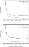 |
Fig. 5 5-σ background sensitivity curves derived from speckle images taken with NESSI for TOI-5153 (top panel) and NGTS-20 (bottom panel) showing no bright companion (∆mag < 4) from 0.2 to 1.2 arcsec. |
Stellar properties and stellar parameters derived with the spectral synthesis method.
3.2 Radial velocity analysis
We first ran an analysis on the radial velocity dataset to find evidence for a periodic signal in the data. We used the kima software package (Faria et al. 2018) to model both radial velocity datasets. kima uses Bayesian inference to model radial velocity series as a sum of Keplerians, where different instruments can be included thanks to the free radial velocity offset between them. Kima also allows to have the number of planets as a free parameter. We chose a uniform prior of between zero and one for the number of planets. The parameters governing the planetary orbit and the priors used in the fit are summarized in Table A.1.
For both systems, there is clear evidence for one periodic signal as the ratio between the number of posterior samples for the one-planet model over the zero-planet model is superior to 150. The orbital period is also clearly defined in both cases: at  days for TOI-5153 and
  days for NGTS-20. The radial velocity time series and their associated generalized Lomb-Scargle periodograms are presented in Fig. 3 for TOI-5153 and in Fig. 4 for NGTS-20.
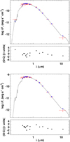 |
Fig. 6 Spectral energy distributions and associated residuals for TOI-5153 (top panel) and NGTS-20 (bottom panel). Red symbols represent the observed photometric measurements, where the horizontal bars represent the effective width of the passband. Blue symbols are the model fluxes from the best-fit Kurucz atmosphere model (black). |
3.3 Joint analysis
We perform the joint analysis of the photometric and radial-velocity data with the software package juliet (Espinoza et al. 2019). Juliet uses Bayesian inference to model a set number of planetary signals. For the light curve modeling, juliet uses batman (Kreidberg 2015) to model the planetary transit, and the stellar activity as well as instrumental systematics can be taken into account with Gaussian processes (Gibson 2014) or simpler parametric functions. For the radial velocity modeling, juliet uses radvel (Fulton et al. 2018) and stellar activity signal can also be modeled with Gaussian processes. We chose to use the nested sampling method dynesty (Speagle 2019) implemented in juliet. Several instruments can be taken into account with radial velocity offsets between them.
For TOI-5153, only two planetary transits have been observed with TESS. In the case of a duo-transit, the solution in orbital period is a discontinuous space where several period aliases can explain the two observed transits. Setting a broad uniform prior on the orbital period leads the algorithm to only explore parts of the parameter space, usually around one or two of the period aliases. To overcome this difficulty, we can combine several dynesty runs and obtain a more complete picture of the posterior distribution. We note that the period alias with the highest likelihood corresponds to the orbital period also found with the analysis of the radial-velocity data.
We therefore chose to set a Normal prior with a width of 0.1 days on the orbital period for the joint fit. In order to confirm the correct period alias, we ran the joint modeling with six sets of priors. We tested the three period aliases closest to the orbital period found with the radial velocity fit (20.1 days). For each period alias prior, we either fixed the eccentricity to zero or we let the eccentricity be a free parameter.
For NGTS-20, the TESS light curves displayed one transit and we obtained two additional transits with NGTS; the solution in orbital period is therefore well constrained and does not present period aliases. For both stars, the parameters and their prior distributions used for the joint fit are listed in Table B.1. Both targets were analyzed with the same choice of model parameters. For the planet, we have the orbital period, mid-transit time, impact parameter, and planet-to-star radius ratio. The eccentricity and argument of periastron are used directly as model parameters and the eccentricity is governed by a Beta prior as detailed in Kipping (2014).
We chose to use the stellar density as a parameter instead of the scaled semi-major axis (a/R*). The Normal prior on stellar density is informed by the stellar analysis which allowed us to derive precise masses and radii and their associated errors. TESS and NGTS have slightly different bandpasses which we modeled by setting two sets of limb-darkening parameters. We chose a quadratic limb darkening parameterized as (q1, q2) in order to efficiently sample the parameter space (Kipping 2013). Additional jitters and offsets are taken into account in the modeling. As the TESS sectors are two years apart and NGTS observed the two transits of NGTS-20 with different number of cameras, we have a set of four jitters and offsets for NGTS-20. For TOI-5153, we have a set of two jitters and offsets as only two TESS light curves are available.
For the radial velocity model, the semi-amplitude is one of parameters and each spectrograph has a separate offset and jitter parameters. For both targets, we used the nested sampling algorithm implemented in juliet, dynesty: each fit was done with 1000 live points and until the estimated uncertainty on the log-evidence is smaller than 0.1.
Photometric variability and radial velocity jitter can be accounted for either through linear models against any parameters or through Gaussian processes. The TESS light curves show small levels of stellar variability both in the SAP and PDCSAP fluxes. The first NGTS light curve of NGTS-20 shows a drop in flux after the end of the first transit, as visible in Fig. 2. We tried to decorrelate this feature against relevant parameters extracted from the NGTS observations (e.g., time, airmass, peak flux) but we were unable to find a combination of linear models which would model it. We chose to model correlated noise in all datasets with a Gaussian process using an approximate Matern kernel implemented via celerite (Foreman-Mackey et al. 2017).
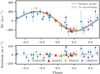 |
Fig. 7 Radial velocities from CORALIE (blue dots), HARPS (red triangles), FEROS (orange crosses), and CHIRON (purple stars) for TOI-5153. Median Keplerian model is plotted as a gray line along with its corresponding 1σ uncertainty (gray shaded area). |
Model comparison based on the log-evidence values (ln Z) for TOI-5153.
4 Results
We present the final parameters derived from the joint analysis of TOI-5153 b in Sect. 4.1 and NGTS-20 b in Sect. 4.2. We compute a first estimate of the heavy element content for both planets in Sect. 4.3.
4.1 TOI-5153
For TOI-5153 we find that the best solution from the joint fit corresponds to the orbital period of 20.33 days. The log-evidence values for the six joint fits are shown in Table 4. The highest evidence model favors a noncircular orbit with an eccentricity of  . The planet has a radius of
  RJup for a mass of
  MJup. The semi-major axis is equal to
  au.
au.
Figure 7 presents the phase folded radial velocities along with the median radial velocity model. The radial velocity semi-amplitude is equal to  m s−1 . The residuals on the radial velocity are about 129, 76, 33, and 15 ms−1 for CHIRON, CORALIE, FEROS, and HARPS, respectively. After about one year of radial velocity monitoring of the system, we do not see any hint of long-term drift.
Each TESS sector light curve is modeled with a Gaussian process with an amplitude of 270 ppm and 560 ppm and a timescale of 0.9 days and 1.4 days for sectors 6 and 33, respectively. The 30 min binned residuals after model subtraction for the light curve are about 620 ppm for sector 6 and 490 ppm for sector 33. Phase-folded light curves and their corresponding models are shown in Fig. 1. The posterior distributions of the planetary parameters, the stellar density, and the radial velocity semi-amplitude are presented in Fig. C.1. The final parameters of the system can be found in Table 5.
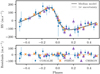 |
Fig. 8 Radial velocities from CORALIE (blue points), FEROS (orange crosses), and CHIRON (purple triangles) for NGTS-20. The median Keplerian model is plotted as a gray line along with its corresponding 1 σ uncertainty (gray shaded area). |
4.2 NGTS-20
NGTS-20 hosts a massive warm Jupiter on a longer period orbit of about 54.19 days. The planet has a mass of  MJup and a radius of
  RJup. The orbital eccentricity is equal to
  andthe semi-majoraxis to
  au.
au.
The radial velocity semi-amplitude is equal to  ms−1 and the residuals are about 30, 40, and 12 ms−1 for CORALIE, CHIRON, and FEROS, respectively. The phase folded radial velocities are presented in Fig. 8. The radial velocity observations of NGTS-20 cover a baseline of two years and there is no hint of long-term drift. The three transits are shown in Fig. 2. The 30 min binned residuals for the TESS light curve are about 390 ppm. The two NGTS light curves show residuals, binned to 30 min, close to 525 ppm for the one camera observation and 130 ppm for the observation with six cameras. Figure C.2 displays the posterior distributions of the planetary parameters along with the stellar density and radial velocity semi-amplitude. The final parameters of the system are listed in Table 5.
4.3 Heavy element content
We estimate the heavy element content of both warm Jupiters by comparing their planetary mass and radius with interior structure models. We used the planetary evolution model completo21 (Mordasini et al. 2012) for the core and the envelope modeling and coupled it with a semi-gray atmospheric model (Guillot 2010). We select the SCvH equations of state (EOS) of hydrogen and helium (H and He) with a He mass fraction of Y = 0.27 (Saumon et al. 1995). As in Thorngren et al. (2016), we model the planet with a planetary core of 10 M⊕. The core is composed of iron and silicates, with an iron mass fraction of 33%. The remaining heavy elements are homogeneously mixed in the H/He envelope. The heavy elements are modeled as water with the AQUA2020 EOS of water (Haldemann et al. 2020).
We run the evolution tracks for both planets from 10 Myr to 8 Gyr, varying the water mass fraction from 0 to 0.25, as shown in Fig. 9. We compute the error on the water mass fraction using a Monte Carlo approach, taking into account the uncertainties on the planetary radius and the stellar age. We choose an average value of  Gyr for the age of NGTS-20. We find that the radius of the planets are well explained with a water mass fraction of
  for TOI-5153b and
  for NGTS-20 b corresponding to a heavy element mass of 133 M⊕ and 104 M⊕, respectively. We varied the planetary mass within the 1σ uncertainty and find no significant changes of the water mass fraction.
We assume that the stellar metallicity scales with the iron abundance ([Fe/H]) derived in Sect. 3.1 as follows: Z* = 0.0142 × 10[Fe/H] (Asplund et al. 2009; Miller & Fortney 2011). The heavy element enrichment (Zp/Z*) is estimated at  for TOI-5153 b and
  for NGTS-20b. We can calculate the heavy element enrichment using Thorngren et al. (2016) relations and we find that Zp/Z* is equal to
  for TOI-5153 b and
  for NGTS-20b. For both planets, our values are in agreement with the estimations derived from Thorngren et al. (2016).
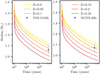 |
Fig. 9 Evolution curves of the planetary radius as a function of time, color coded according to the water mass fraction in the envelope for TOI-5153 b (leftpanel) and NGTS-20 b (rightpanel). |
5 Discussion
The majority of known gas giants with measured masses and radii are hot Jupiters. They have orbital periods of a few days and are subject to strong interactions with their host star, such as tidal interactions (e.g., Valsecchi et al. 2015) and radius inflation mechanisms (e.g., Sestovic et al. 2018; Sarkis et al. 2021; Tilbrook et al. 2021). There is a positive correlation between the planetary radius and the amount of stellar incident flux (Enoch et al. 2012) and only hot Jupiters receiving a level of stellar irradiation lower than 2 × 10⁸ erg s−1 cm−2 are shown to have a radius independent of the stellar irradiation (Demory & Seager 2011). Cooler gas giants, such as TOI-5153 b and NGTS-20b, with equilibrium temperatures of about 900 K and 700 K, should not be affected by radius inflation mechanisms. We can therefore derive precise bulk metallicities based on evolution models (e.g., Thorngren & Fortney 2019). We provide first estimates of the heavy element contents of TOI-5153 b and NGTS-20b. We show that their metal enrichment is in agreement with the mass-metallicity relation and is consistent with planets at long periods with comparable masses (e.g., Dalba et al. 2022). Both planets are excellent probes to help us better understand this relation.
We compare the properties of both planets with the population of known transiting exoplanets. We queried the DACE PlanetS exoplanet catalog database1 on February 10, 2022, and selected exoplanets with mass and radius uncertainties smaller than 25% and 8% respectively. The radius uncertainty is scaled to one-third of the mass uncertainty to have the same impact on the planetary density.
Figure 10 shows that TOI-5153 b and NGTS-20b populate a region of the parameter space where fewer systems have been reported with precise mass and radius. In addition, TOI-5153 b and NGTS-20 b orbit relatively bright stars (Vmag = 11.9 and 11.2) in comparison to the known systems with orbital periods above 20 days. While the Kepler mission was successful at detecting long-period transiting planets, most of these discoveries were made around faint stars (e.g., Wang et al. 2015; Kawahara & Masuda 2019). The follow-up of TESS single-transit candidates allows one to probe the same population of planets around brighter stars (e.g., Eisner et al. 2020; Dalba et al. 2022), which are better suited for follow-up observations.
Figure 11 presents the masses, periods, and eccentricities of warm transiting planets. Despite the small number, we notice that higher mass planets (MP > 3–4 MJ) show higher eccentricities. This trend is reported by Ribas & Miralda-Escudé (2007) for a larger sample of planets detected in radial velocities, where the authors show that the eccentricity distribution of higher mass planets is similar to that of binary stars; hinting that these planets may have formed by pre-stellar cloud fragmentation. TOI-5153 b and NGTS-20 b have similar masses and significantly eccentric orbits with eccentricities of 0.091 ± 0.026 and 0.43 ± 0.02, respectively. Bitsch et al. (2013) showed that the eccentricity of planets with MP < 5 MJ can be damped by the disk. However, Debras et al. (2021) present disk-cavity migration as a possible explanation for eccentricities up to 0.4 for warm Jupiter-mass planets. Another feature that can be seen is that the highest eccentricities do not occur at closer orbital distances. A possible reason for this high-eccentricity cutoff could be tidal circularization by the host star (Adams & Laughlin 2006; Dawson & Johnson 2018). Planetary orbits beyond a threshold in eccentricity and orbital distance circularize before we observe them (Schlecker et al. 2020). Eccentric warm Jupiters like NGTS-20 b can therefore serve as a valuable test bed to study tidal interactions between planets and their host stars.
The eccentricities of both targets, and especially NGTS-20 b, make them interesting candidates for high-eccentricity migration. Eccentric warm Jupiters could be exoplanets caught in the midst of inward migration. The migration would bring them to close-in orbits, and the orbits of the new hot Jupiters would circularize due to stellar tidal forces. However, other scenarios have been put forward, Schlecker et al. (2020) present the discovery of a warm Jupiter on a highly eccentric 15-day orbit (e ~ 0.58); the tidal evolution analysis of this system shows that its current architecture likely resulted from an interaction with an undetected companion rather than an ongoing high-eccentricity migration. High-eccentricity migration is a scenario which can be tested by measuring the spin-orbit of the system. Both targets are suitable for Rossiter-McLaughlin observations. The predicted Rossiter-Mclaughlin effect measured with the classical method is about 40 m s−1 for TOI-5153 b and 16 m s−1 for NGTS-20 b (Eq. (40) from Winn 2010). The Rossiter-Mclaughlin effect is large enough for the spin-orbit angle of the system to be measured with current high-resolution spectrographs.
Derived parameters for TOI-5153 and NGTS-20 systems.
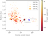 |
Fig. 10 Radius-period diagram for the population of transiting giant planets (MP > 0.2 MJ) with mass and radius uncertainties smaller than 25% and 8%, respectively. The size of the points is proportional to the planetary mass and the V band magnitude is color coded. TOI-5153 b is circled in black and NGTS-20 b in blue. |
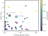 |
Fig. 11 Mass-period diagram for the population of transiting giant planets (MP > 0.2 MJ and P > 10 days) with mass and radius uncertainties smaller than 25% and 8% respectively, color-coded as a function of orbital eccentricity. TOI-5153 b is circled in black and NGTS-20 b in blue. |
6 Conclusions
We report the discovery of two transiting massive warm Jupiters around the bright and metal-rich stars TOI-5153 and NGTS-20. TOI-5153 hosts a planet on a 20.33 days period with a planetary mass of 3.26 ± 0.18 MJ and planetary radius of 1.06 ± 0.04RJ. The orbit of the planet has an eccentricity of 0.091 ± 0.026. NGTS-20 hosts a longer period planet with an orbital period of 54.19 days. The planet has a radius of 1.07 ± 0.04 RJ; a planetary mass of 2.98 ± 0.16 MJ, and presents an eccentric orbit with an eccentricity of 0.43 ± 0.02. We show that both planets are metal enriched and their heavy element content is consistent with the mass-metallicity relation of gas giants. We used TESS photometry to identify single-transit candidates which were then followed up with ground-based photometric and spectroscopic instruments in order to confirm the planetary nature of the transiting objects. Both warm Jupiters orbit bright stars and are ideal targets for additional observations in order to measure the spin-orbit alignment of these systems. These exoplanets show that our selection of targets with single and duo transits and subsequent radial velocity follow-up are successful and we expect more discoveries of long-period transiting planets over the coming years.
Acknowledgements
This work has been carried out within the framework of the National Centre of Competence in Research PlanetS supported by the Swiss National Science Foundation under grants 51NF40_182901 and 51NF40_205606. The authors acknowledge the financial support of the SNSF. M.L. acknowledges support of the Swiss National Science Foundation under grant number PCEFP2194576. The NGTS facility is operated by the consortium institutes with support from the UK Science and Technology Facilities Council (STFC) under projects ST/M001962/1 and ST/S002642/1. The contributions at the University of Warwick by P.J.W., R.G.W., D.R.A., and S.G. have been supported by STFC through consolidated grants ST/L000733/1 and ST/P000495/1. R.B. acknowledges support from FONDECYT Project 11200751 and from ANID - Millennium Science Initiative. D.D. acknowledges support from the TESS Guest Investigator Program grants 80NSSC21K0108 and 80NSSC22K0185, and NASA Exoplanet Research Program grant 18-2XRP18_2-0136. Some of the observations in this paper made use of the NN-EXPLORE Exoplanet and Stellar Speckle Imager (NESSI). NESSI was funded by the NASA Exoplanet Exploration Program and the NASA Ames Research Center. NESSI was built at the Ames Research Center by Steve B. Howell, Nic Scott, Elliott P. Horch, and Emmett Quigley. G.Z. thanks the support of the ARC DECRA program DE210101893. A.J., F.R., and P.T. acknowledge support from ANID – Millennium Science Initiative – ICN12_009 and from FONDECYT project 1210718. The results reported herein benefited from collaborations and/or information exchange within the program “Alien Earths” (supported by the National Aeronautics and Space Administration under agreement no. 80NSSC21K0593) for NASA’s Nexus for Exoplanet System Science (NExSS) research coordination network sponsored by NASA s Science Mission Directorate. J.S.J. gratefully acknowledges support by FONDECYT grant 1201371 and from the ANID BASAL projects ACE210002 and FB210003. M.N.G. acknowledges support from the European Space Agency (ESA) as an ESA Research Fellow. The work performed by HPO has been carried out within the framework of the NCCR PlanetS supported by the Swiss National Science Foundation. E.G. gratefully acknowledges support from the David and Claudia Harding Foundation in the form of a Winton Exoplanet Fellowship. T.T. acknowledges support by the DFG Research Unit FOR 2544 “Blue Planets around Red Stars” project no. KU 3625/2-1. T.T. further acknowledges support by the BNSF program “VIHREN-2021” project No. K∏-06-,Z];B/5. J.I.V. acknowledges support of CONICYT-PFCHA/Doctorado Nacional-21191829. The authors acknowledge the use of public TESS data from pipelines at the TESS Science Office and at the TESS Science Processing Operations Centre. This paper includes data collected with the TESS mission obtained from the MAST data archive at the Space Telescope Science Institute (STScI). Funding for the TESS mission is provided by the NASA Explorer program. STScI is operated by the Association of Universities for Research in Astronomy, Inc., under NASA contract NAS5-26555. This work made use of tpfplotter by J. Lillo-Box (publicly available in www.github.com/jlillo/tpfplotter), which also made use of the python packages astropy, lightkurve, matplotlib and numpy. This publication makes use of The Data & Analysis Center for Exoplanets (DACE), which is a facility based at the University of Geneva (CH) dedicated to extra-solar planets data visualisation, exchange and analysis. DACE is a platform of the Swiss National Centre of Competence in Research (NCCR) PlanetS, federating the Swiss expertise in Exoplanet research. The DACE platform is available at https://dace.unige.ch.
Appendix A Radial velocity modeling priors
Priors for the fit of the radial velocities alone.
Appendix B Joint modeling priors
Priors for the joint modeling of photometric and radial velocity data.
Appendix C Joint modeling posterior distributions
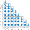 |
Fig. C.1 Posterior distributions of fitted parameters for TOI-5153 b along with the stellar density (ρ) and radial velocity semi-amplitude (K). |
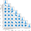 |
Fig. C.2 Posterior distributions of fitted parameters for NGTS-20 b along with the stellar density (ρ) and radial velocity semi-amplitude (K). |
References
- Adams, F. C., & Laughlin, G. 2006, ApJ, 649, 1004 [Google Scholar]
- Albrecht, S., Winn, J. N., Johnson, J. A., et al. 2012, ApJ, 757, 18 [NASA ADS] [CrossRef] [Google Scholar]
- Alibert, Y., Mousis, O., Mordasini, C., & Benz, W. 2005, ApJ, 626, L57 [NASA ADS] [CrossRef] [Google Scholar]
- Aller, A., Lillo-Box, J., Jones, D., Miranda, L. F., & Barceló Forteza, S. 2020, A&A, 635, A128 [NASA ADS] [CrossRef] [EDP Sciences] [Google Scholar]
- Asplund, M., Grevesse, N., Sauval, A. J., & Scott, P. 2009, ARA&A, 47, 481 [NASA ADS] [CrossRef] [Google Scholar]
- Baruteau, C., Crida, A., Paardekooper, S. J., et al. 2014, Protostars and Planets VI, eds. H. Beuther, R. S. Klessen, C. P. Dullemond, & T. Henning (Tucson: University of Arizona Press), 914, 667 [Google Scholar]
- Baxter, C., Désert, J.-M., Tsai, S.-M., et al. 2021, A&A, 648, A127 [NASA ADS] [CrossRef] [EDP Sciences] [Google Scholar]
- Bianchi, L., Shiao, B., & Thilker, D. 2017, ApJS, 230, 24 [Google Scholar]
- Bitsch, B., Crida, A., Libert, A.-S., & Lega, E. 2013, A&A, 555, A124 [NASA ADS] [CrossRef] [EDP Sciences] [Google Scholar]
- Blanco-Cuaresma, S., Soubiran, C., Heiter, U., & Jofré, P. 2014, A&A, 569, A111 [CrossRef] [EDP Sciences] [Google Scholar]
- Brahm, R., Jordán, A., & Espinoza, N. 2017, PASP, 129, 034002 [Google Scholar]
- Buchhave, L. A., Bakos, G. Á., Hartman, J. D., et al. 2010, ApJ, 720, 1118 [NASA ADS] [CrossRef] [Google Scholar]
- Buchhave, L. A., Latham, D. W., Johansen, A., et al. 2012, Nature, 486, 375 [NASA ADS] [Google Scholar]
- Buchhave, L. A., Bizzarro, M., Latham, D. W., et al. 2014, Nature, 509, 593 [Google Scholar]
- Coleman, G. A. L., & Nelson, R. P. 2016, MNRAS, 460, 2779 [NASA ADS] [CrossRef] [Google Scholar]
- Cooke, B. F., Pollacco, D., West, R., McCormac, J., & Wheatley, P. J. 2018, A&A, 619, A175 [NASA ADS] [CrossRef] [EDP Sciences] [Google Scholar]
- Dalba, P. A., Kane, S. R., Dragomir, D., et al. 2022, AJ, 163, 61 [NASA ADS] [CrossRef] [Google Scholar]
- Dawson, R. I., & Johnson, J. A. 2018, ARA&A, 56, 175 [Google Scholar]
- Debras, F., Baruteau, C., & Donati, J.-F. 2021, MNRAS, 500, 1621 [Google Scholar]
- Demory, B.-O., & Seager, S. 2011, ApJS, 197, 12 [NASA ADS] [CrossRef] [Google Scholar]
- Donati, J.-F., Semel, M., Carter, B. D., Rees, D. E., & Cameron, A. C. 1997, MNRAS, 291, 658 [Google Scholar]
- Eisner, N. L., Barragán, O., Aigrain, S., et al. 2020, MNRAS, 494, 750 [NASA ADS] [CrossRef] [Google Scholar]
- Enoch, B., Collier Cameron, A., & Horne, K. 2012, A&A, 540, A99 [NASA ADS] [CrossRef] [EDP Sciences] [Google Scholar]
- Espinoza, N., Kossakowski, D., & Brahm, R. 2019, MNRAS, 490, 2262 [Google Scholar]
- Fabrycky, D., & Tremaine, S. 2007, ApJ, 669, 1298 [NASA ADS] [CrossRef] [Google Scholar]
- Faria, J. P., Santos, N. C., Figueira, P., & Brewer, B. J. 2018, J. Open Source Softw., 3, 487 [NASA ADS] [CrossRef] [Google Scholar]
- Foreman-Mackey, D., Agol, E., Ambikasaran, S., & Angus, R. 2017, AJ, 154, 220 [Google Scholar]
- Fulton, B. J., Petigura, E. A., Blunt, S., & Sinukoff, E. 2018, PASP, 130, 044504 [Google Scholar]
- Fürész, G. 2008, PhD thesis, University of Szeged, Hungary [Google Scholar]
- Gaia Collaboration (G. Brown, A. G. A., et al.) 2021, A&A, 649, A1 [NASA ADS] [CrossRef] [EDP Sciences] [Google Scholar]
- Gibson, N. P. 2014, MNRAS, 445, 3401 [NASA ADS] [CrossRef] [Google Scholar]
- Gill, S., Bayliss, D., Cooke, B. F., et al. 2020a, MNRAS, 491, 1548 [Google Scholar]
- Gill, S., Wheatley, P. J., Cooke, B. F., et al. 2020b, ApJ, 898, L11 [Google Scholar]
- Gill, S., Ulmer-Moll, S., Wheatley, P. J., et al. 2022, MNRAS, 513, 1785 [NASA ADS] [CrossRef] [Google Scholar]
- Goldreich, P., & Tremaine, S. 1980, ApJ, 241, 425 [Google Scholar]
- Guerrero, N. M., Seager, S., Huang, C. X., et al. 2021, ApJS, 254, 39 [NASA ADS] [CrossRef] [Google Scholar]
- Guillot, T. 2010, A&A, 520, A27 [NASA ADS] [CrossRef] [EDP Sciences] [Google Scholar]
- Gustafsson, B., Edvardsson, B., Eriksson, K., et al. 2008, A&A, 486, 951 [NASA ADS] [CrossRef] [EDP Sciences] [Google Scholar]
- Haldemann, J., Alibert, Y., Mordasini, C., & Benz, W. 2020, A&A, 643, A105 [NASA ADS] [CrossRef] [EDP Sciences] [Google Scholar]
- Henden, A., & Munari, U. 2014, Contrib. Astron. Observ. Skalnate Pleso, 43, 518 [NASA ADS] [Google Scholar]
- Høg, E., Fabricius, C., Makarov, V. V., et al. 2000, A&A, 355, L27 [Google Scholar]
- Howell, S. B., Everett, M. E., Sherry, W., Horch, E., & Ciardi, D. R. 2011, AJ, 142, 19 [Google Scholar]
- Huang, C. X., Vanderburg, A., Pál, A., et al. 2020a, Res. Notes Am. Astron. Soc., 4, 204 [Google Scholar]
- Huang, C. X., Vanderburg, A., Pál, A., et al. 2020b, Res. Notes Am. Astron. Soc., 4, 206 [Google Scholar]
- Jenkins, J. M., Twicken, J. D., McCauliff, S., et al. 2016, SPIE Conf. Ser., 9913, 99133E [Google Scholar]
- Jones, M. I., Brahm, R., Espinoza, N., et al. 2019, A&A, 625, A16 [NASA ADS] [CrossRef] [EDP Sciences] [Google Scholar]
- Kaufer, A., Stahl, O., Tubbesing, S., et al. 1999, The Messenger, 95, 8 [Google Scholar]
- Kawahara, H., & Masuda, K. 2019, AJ, 157, 218 [NASA ADS] [CrossRef] [Google Scholar]
- Kipping, D. M. 2013, MNRAS, 435, 2152 [Google Scholar]
- Kipping, D. M. 2014, MNRAS, 444, 2263 [NASA ADS] [CrossRef] [Google Scholar]
- Kreidberg, L. 2015, PASP, 127, 1161 [Google Scholar]
- Kurucz, R. L. 1992, The Stellar Populations of Galaxies, eds. B. Beatriz & R. Alvio, 149, 225 [CrossRef] [Google Scholar]
- Lendl, M., Bouchy, F., Gill, S., et al. 2020, MNRAS, 492, 1761 [NASA ADS] [CrossRef] [Google Scholar]
- Madhusudhan, N., Crouzet, N., McCullough, P. R., Deming, D., & Hedges, C. 2014, ApJ, 791, L9 [Google Scholar]
- Mamajek, E. E., & Hillenbrand, L. A. 2008, ApJ, 687, 1264 [Google Scholar]
- Mayor, M., Pepe, F., Queloz, D., et al. 2003, The Messenger, 114, 20 [NASA ADS] [Google Scholar]
- Melo, C., Santos, N. C., Gieren, W., et al. 2007, A&A, 467, 721 [NASA ADS] [CrossRef] [EDP Sciences] [Google Scholar]
- Miller, N., & Fortney, J. J. 2011, ApJ, 736, L29 [NASA ADS] [CrossRef] [Google Scholar]
- Montalto, M., Borsato, L., Granata, V., et al. 2020, MNRAS, 498, 1726 [NASA ADS] [CrossRef] [Google Scholar]
- Mordasini, C., Alibert, Y., Klahr, H., & Henning, T. 2012, A&A, 547, A111 [NASA ADS] [CrossRef] [EDP Sciences] [Google Scholar]
- Mordasini, C., Klahr, H., Alibert, Y., Miller, N., & Henning, T. 2014, A&A, 566, A141 [NASA ADS] [CrossRef] [EDP Sciences] [Google Scholar]
- Mordasini, C., van Boekel, R., Mollière, P., Henning, T., & Benneke, B. 2016, ApJ, 832, 41 [Google Scholar]
- Osborn, H. P., Armstrong, D. J., Brown, D. J. A., et al. 2016, MNRAS, 457, 2273 [NASA ADS] [CrossRef] [Google Scholar]
- Osborn, H. P., Bonfanti, A., Gandolfi, D., et al. 2022, A&A, 664, A156 [NASA ADS] [CrossRef] [EDP Sciences] [Google Scholar]
- Pepe, F., Mayor, M., Rupprecht, G., et al. 2002, The Messenger, 110, 9 [NASA ADS] [Google Scholar]
- Petrovich, C., & Tremaine, S. 2016, ApJ, 829, 132 [NASA ADS] [CrossRef] [Google Scholar]
- Petrovich, C., Tremaine, S., & Rafikov, R. 2014, ApJ, 786, 101 [NASA ADS] [CrossRef] [Google Scholar]
- Queloz, D., Mayor, M., Udry, S., et al. 2001, The Messenger, 105, 1 [NASA ADS] [Google Scholar]
- Rasio, F. A., & Ford, E. B. 1996, Science, 274, 954 [Google Scholar]
- Ribas, I., & Miralda-Escudé, J. 2007, A&A, 464, 779 [NASA ADS] [CrossRef] [EDP Sciences] [Google Scholar]
- Ricker, G. R., Winn, J. N., Vanderspek, R., et al. 2015, J. Astron. Telescopes Instrum. Syst., 1, 014003 [Google Scholar]
- Santerne, A., Moutou, C., Tsantaki, M., et al. 2016, A&A, 587, A64 [NASA ADS] [CrossRef] [EDP Sciences] [Google Scholar]
- Sarkis, P., Mordasini, C., Henning, T., Marleau, G. D., & Mollière, P. 2021, A&A, 645, A79 [NASA ADS] [CrossRef] [EDP Sciences] [Google Scholar]
- Saumon, D., Chabrier, G., & van Horn, H. M. 1995, ApJS, 99, 713 [NASA ADS] [CrossRef] [Google Scholar]
- Schanche, N., Pozuelos, F. J., Günther, M. N., et al. 2022, A&A, 657, A45 [NASA ADS] [CrossRef] [EDP Sciences] [Google Scholar]
- Schlecker, M., Kossakowski, D., Brahm, R., et al. 2020, AJ, 160, 275 [Google Scholar]
- Schlegel, D. J., Finkbeiner, D. P., & Davis, M. 1998, ApJ, 500, 525 [Google Scholar]
- Scott, N. J., Howell, S. B., Horch, E. P., & Everett, M. E. 2018, PASP, 130, 054502 [Google Scholar]
- Sestovic, M., Demory, B.-O., & Queloz, D. 2018, A&A, 616, A76 [NASA ADS] [CrossRef] [EDP Sciences] [Google Scholar]
- Showman, A. P., Tan, X., & Parmentier, V. 2020, Space Sci. Rev., 216, 139 [Google Scholar]
- Sing, D. K., Fortney, J. J., Nikolov, N., et al. 2016, Nature, 529, 59 [Google Scholar]
- Skrutskie, M. F., Cutri, R. M., Stiening, R., et al. 2006, AJ, 131, 1163 [NASA ADS] [CrossRef] [Google Scholar]
- Speagle, J. S. 2019, arXiv e-prints [arXiv:1909.12313] [Google Scholar]
- Stassun, K. G., & Torres, G. 2016, AJ, 152, 180 [Google Scholar]
- Stassun, K. G., & Torres, G. 2021, ApJ, 907, L33 [NASA ADS] [CrossRef] [Google Scholar]
- Stassun, K. G., Collins, K. A., & Gaudi, B. S. 2017, AJ, 153, 136 [Google Scholar]
- Stassun, K. G., Corsaro, E., Pepper, J. A., & Gaudi, B. S. 2018, AJ, 155, 22 [Google Scholar]
- Teske, J. K., Thorngren, D., Fortney, J. J., Hinkel, N., & Brewer, J. M. 2019, AJ, 158, 239 [NASA ADS] [CrossRef] [Google Scholar]
- Thorngren, D., & Fortney, J. J. 2019, ApJ, 874, L31 [Google Scholar]
- Thorngren, D. P., Fortney, J. J., Murray-Clay, R. A., & Lopez, E. D. 2016, ApJ, 831, 64 [NASA ADS] [CrossRef] [Google Scholar]
- Tilbrook, R. H., Burleigh, M. R., Costes, J. C., et al. 2021, MNRAS, 504, 6018 [NASA ADS] [CrossRef] [Google Scholar]
- Tokovinin, A., Fischer, D. A., Bonati, M., et al. 2013, PASP, 125, 1336 [NASA ADS] [CrossRef] [Google Scholar]
- Torres, G., Andersen, J., & Giménez, A. 2010, A&AR, 18, 67 [NASA ADS] [CrossRef] [Google Scholar]
- Udry, S., Mayor, M., & Santos, N. C. 2003, A&A, 407, 369 [NASA ADS] [CrossRef] [EDP Sciences] [Google Scholar]
- Valsecchi, F., Rappaport, S., Rasio, F. A., Marchant, P., & Rogers, L. A. 2015, ApJ, 813, 101 [NASA ADS] [CrossRef] [Google Scholar]
- Villanueva, S., Jr., Dragomir, D., & Gaudi, B. S. 2019, AJ, 157, 84 [NASA ADS] [CrossRef] [Google Scholar]
- Wang, J., Fischer, D. A., Barclay, T., et al. 2015, ApJ, 815, 127 [NASA ADS] [CrossRef] [Google Scholar]
- Wang, S., Jones, M., Shporer, A., et al. 2019, AJ, 157, 51 [Google Scholar]
- Wheatley, P. J., West, R. G., Goad, M. R., et al. 2018, MNRAS, 475, 4476 [Google Scholar]
- Winn, J. N. 2010, arXiv e-prints [arXiv:1001.2010] [Google Scholar]
- Wittenmyer, R. A., O’Toole, S. J., Jones, H. R. A., et al. 2010, ApJ, 722, 1854 [NASA ADS] [CrossRef] [Google Scholar]
- Wong, M. H., Mahaffy, P. R., Atreya, S. K., Niemann, H. B., & Owen, T. C. 2004, Icarus, 171, 153 [Google Scholar]
- Wright, E. L., Eisenhardt, P. R. M., Mainzer, A. K., et al. 2010, AJ, 140, 1868 [Google Scholar]
- Wu, Y., & Lithwick, Y. 2011, ApJ, 735, 109 [Google Scholar]
- Wyttenbach, A., Lovis, C., Ehrenreich, D., et al. 2017, A&A, 602, A36 [NASA ADS] [CrossRef] [EDP Sciences] [Google Scholar]
All Tables
Stellar properties and stellar parameters derived with the spectral synthesis method.
All Figures
|
Fig. 1 Top: photometric observations of TOI-5153 from TESS sector 6 at 30 min cadence (orange dots, left panel) and sector 33 at 10 min cadence (green dots, middle panel) with full median models (orange and green lines), and Gaussian process models (black line). The right panel shows the detrended and phase-folded data from both sectors (orange and green dots) with the phase-folded transit model in black. Bottom: each panel shows the residuals in parts per million between the full model and the respective light curve. |
| In the text | |
|
Fig. 2 Top: photometric observations of NGTS-20 from TESS sector 4 at 30 min cadence (left panel) and NGTS binned at two-minute cadence {middle and right panels). In each panel, the data are shown are colored dots (orange, green, and red), the full model is represented with a line of the same color, and the Gaussian process model is shown as a gray line. Bottom: each panel shows the residuals in parts per million between the full model and the respective light curve. |
| In the text | |
|
Fig. 3 Top: time series of the radial velocities from CORALIE (blue dots), FEROS (orange crosses), HARPS (red triangles), and CHIRON (purple stars) for TOI-5153. Bottom: generalized Lomb-Scargle periodogram of the radial velocities. The highest peak corresponds to a period of about 20.1 days. |
| In the text | |
|
Fig. 4 Top: time series of the radial velocities from CORALIE (blue dots), FEROS (orange crosses), and CHIRON (purple triangles) for NGTS-20. Bottom: generalized Lomb-Scargle periodogram of the radial velocities. The highest peak corresponds to a period of about 53.5 days. |
| In the text | |
|
Fig. 5 5-σ background sensitivity curves derived from speckle images taken with NESSI for TOI-5153 (top panel) and NGTS-20 (bottom panel) showing no bright companion (∆mag < 4) from 0.2 to 1.2 arcsec. |
| In the text | |
|
Fig. 6 Spectral energy distributions and associated residuals for TOI-5153 (top panel) and NGTS-20 (bottom panel). Red symbols represent the observed photometric measurements, where the horizontal bars represent the effective width of the passband. Blue symbols are the model fluxes from the best-fit Kurucz atmosphere model (black). |
| In the text | |
|
Fig. 7 Radial velocities from CORALIE (blue dots), HARPS (red triangles), FEROS (orange crosses), and CHIRON (purple stars) for TOI-5153. Median Keplerian model is plotted as a gray line along with its corresponding 1σ uncertainty (gray shaded area). |
| In the text | |
|
Fig. 8 Radial velocities from CORALIE (blue points), FEROS (orange crosses), and CHIRON (purple triangles) for NGTS-20. The median Keplerian model is plotted as a gray line along with its corresponding 1 σ uncertainty (gray shaded area). |
| In the text | |
|
Fig. 9 Evolution curves of the planetary radius as a function of time, color coded according to the water mass fraction in the envelope for TOI-5153 b (leftpanel) and NGTS-20 b (rightpanel). |
| In the text | |
|
Fig. 10 Radius-period diagram for the population of transiting giant planets (MP > 0.2 MJ) with mass and radius uncertainties smaller than 25% and 8%, respectively. The size of the points is proportional to the planetary mass and the V band magnitude is color coded. TOI-5153 b is circled in black and NGTS-20 b in blue. |
| In the text | |
|
Fig. 11 Mass-period diagram for the population of transiting giant planets (MP > 0.2 MJ and P > 10 days) with mass and radius uncertainties smaller than 25% and 8% respectively, color-coded as a function of orbital eccentricity. TOI-5153 b is circled in black and NGTS-20 b in blue. |
| In the text | |
|
Fig. C.1 Posterior distributions of fitted parameters for TOI-5153 b along with the stellar density (ρ) and radial velocity semi-amplitude (K). |
| In the text | |
|
Fig. C.2 Posterior distributions of fitted parameters for NGTS-20 b along with the stellar density (ρ) and radial velocity semi-amplitude (K). |
| In the text | |
Current usage metrics show cumulative count of Article Views (full-text article views including HTML views, PDF and ePub downloads, according to the available data) and Abstracts Views on Vision4Press platform.
Data correspond to usage on the plateform after 2015. The current usage metrics is available 48-96 hours after online publication and is updated daily on week days.
Initial download of the metrics may take a while.