| Issue |
A&A
Volume 664, August 2022
|
|
|---|---|---|
| Article Number | A98 | |
| Number of page(s) | 19 | |
| Section | Stellar structure and evolution | |
| DOI | https://doi.org/10.1051/0004-6361/202243707 | |
| Published online | 10 August 2022 | |
Apsidal motion in massive eccentric binaries: The case of CPD-41° 7742, and HD 152218 revisited
1
Space Sciences, Technologies and Astrophysics Research (STAR) Institute, Université de Liège, Allée du 6 Août, 19c, Bât B5c, 4000 Liège, Belgium
e-mail: sophie.rosu@uliege.be
2
Physics Department, Vrije Universiteit Brussel, Pleinlaan 2, 1050 Brussels, Belgium
Received:
4
April
2022
Accepted:
6
May
2022
Context. This paper is part of a study of the apsidal motion in close eccentric massive binary systems, which aims to constrain the internal structure of the stars. We focus on the binary CPD-41° 7742 and briefly revisit the case of HD 152218.
Aims. Independent studies of CPD-41° 7742 in the past showed large discrepancies in the longitude of periastron of the orbit, hinting at the presence of apsidal motion. We here perform a consistent analysis of all observational data, explicitly accounting for the rate of change of the longitude of periastron.
Methods. We make use of the extensive set of spectroscopic and photometric observations of CPD-41° 7742 to infer values for the fundamental parameters of the stars and of the binary. Applying a disentangling method to the spectra allows us to simultaneously derive the radial velocities (RVs) at the times of observation and reconstruct the individual spectra of the stars. The spectra are analysed by means of the CMFGEN model atmosphere code to determine the stellar properties. We determine the apsidal motion rate in two ways: First, we complement our RVs with those reported in the literature, and, second, we use the phase shifts between the primary and secondary eclipses. The light curves are further analysed by means of the Nightfall code to constrain the orbital inclination and, thereby, the stellar masses. Stellar structure and evolution models are then constructed with the Clés code for the two stars with the constraints provided by the observations. Different prescriptions for the mixing inside the stars are adopted in the models. Newly available photometric data of HD 152218 are analysed, and stellar structure and evolution models are built for the system as for CPD-41° 7742.
Results. The binary system CPD-41° 7742, made of an O9.5 V primary (MP = 17.8 ± 0.5 M⊙, RP = 7.57 ± 0.09 R⊙, Teff, P = 31 800 ± 1000 K, Lbol,P = 5.28−0.68+0.67 × 10⁴ L⊙) and a B1–2 V secondary (MS = 10.0 ± 0.3 M⊙, RS = 4.29−0.06+0.04 R⊙, Teff, S = 24 098 ± 1000 K, Lbol,S = 5.58−0.94+0.93 × 10³ L⊙), displays apsidal motion at a rate of 15.°38−0.51+0.42 yr−1. Initial masses of 18.0 ± 0.5 M⊙ and 9.9 ± 0.3 M⊙ are deduced for the primary and secondary stars, respectively, and the binary’s age is estimated to be 6.8 ± 1.4 Myr. Regarding HD 152218, initial masses of 20.6 ± 1.5 and 15.5 ± 1.1 M⊙ are deduced for the primary and secondary stars, respectively, and the binary’s age of 5.2 ± 0.8 Myr is inferred.
Conclusions. Our analysis of the observational data of CPD-41° 7742 that explicitly accounts for the apsidal motion allows us to explain the discrepancy in periastron longitudes pointed out in past studies of this binary system. The age estimates are in good agreement with estimates obtained for other massive binaries in NGC 6231. This study confirms the need for enhanced mixing in the stellar evolution models of the most massive stars to reproduce the observational stellar properties; this points towards larger convective cores than usually considered.
Key words: binaries: eclipsing / stars: evolution / stars: individual: CPD-41° 7742 / stars: individual: HD 152218 / stars: massive / binaries: spectroscopic
© S. Rosu et al. 2022
 Open Access article, published by EDP Sciences, under the terms of the Creative Commons Attribution License (https://creativecommons.org/licenses/by/4.0), which permits unrestricted use, distribution, and reproduction in any medium, provided the original work is properly cited.
This article is published in open access under the Subscribe-to-Open model. Subscribe to A&A to support open access publication.
1. Introduction
The high incidence of O-type binary systems in the young open cluster NGC 6231 (Sana et al. 2008, and references therein) makes this cluster, located at the core of the Sco OB1 association, an interesting target for the study of massive star structure and evolution. Stars more massive than 8 M⊙ appear to be more concentrated in the cluster core (Kuhn et al. 2017). The ages of low-mass pre-main-sequence stars in NGC 6231 range between 1 and 7 Myr, with a small peak near 3 Myr (Sana et al. 2007; Sung et al. 2013). More recently, the ages of three massive binary systems belonging to the cluster have been assessed: Rauw et al. (2016) derived an age estimate of 5.8 ± 0.6 Myr for HD 152218, Rosu et al. (2020a) derived an age estimate of 5.25 ± 0.14 Myr for HD 152248, and Rosu et al. (2022) derived an age estimate of 9.5 ± 0.6 Myr for HD 152219, though the authors indicated that this latter age was probably overestimated. The common feature between these three studies is that the age is determined based on the analysis of the apsidal motion of these binaries. Indeed, the apsidal motion rate in an eccentric binary depends upon the internal structure constant of the stars, that is to say, the density stratification between the stellar core and the external layers, and hence, the evolutionary stage (i.e. the age) of the stars composing the system. This paper follows the path of these three studies and concentrates on a fourth massive binary system belonging to NGC 6231, namely CPD-41° 7742. We also briefly revisit the HD 152218 system in light of the newly available photometric data and stellar evolution codes that have been improved since our first analysis of this system (Rauw et al. 2016).
In a broader context, the measurement of the apsidal motion rate in eccentric eclipsing binaries offers a unique opportunity to gain direct insight into the internal structure of the stars. Complemented by the fundamental stellar properties obtained from the light curves and from spectroscopy, the apsidal motion rate yields additional constraints that can be used to perform critical tests of stellar structure and evolution models (e.g. Claret & Torres 2019; Claret et al. 2021, and references therein). There has been renewed interest in this field recently thanks to the Transiting Exoplanet Survey Satellite (TESS) mission (Ricker et al. 2015) which provides densely covered light curves of eclipsing binary systems at very high precision (Baroch et al. 2021).
The massive binary CPD-41° 7742 – also known as V 1034 Sco – is the second known eclipsing early-type double-lined spectroscopic (SB2) binary system of NGC 6231, discovered after HD 152248. Struve (1944) was the first to suspect the binarity of CPD-41° 7742. With more data, Hill et al. (1974) derived the first orbital solution for the system (see Table 1) and reported a photometric variability of ΔV = 0.45 mag. The primary star was assigned the spectral type O9 IV by Levato & Malaroda (1980). Levato & Morrell (1983) derived a new orbital solution (see Table 1). Whilst Perry et al. (1990) published additional radial velocity (RV) data points, they did not present any new orbital solution for the system. García & Mermilliod (2001) reported the first evidence of the presence of the secondary star in three out of their eight new medium-resolution spectra. They derived the first SB2 solution of the system (see Table 1). However, Sana et al. (2003) reported errors in the Julian dates of some of the observations of García & Mermilliod (2001), and redetermined the orbital period and the eccentricity of the system based on 34 new data points that complemented the previous literature data available at that time (see Table 1). They determined an O9 III + B1 III spectral classification for the system, even though they claimed that the stars would be main-sequence stars rather than giant stars considering the physical configuration of the system. Sana et al. (2005) reassessed the spectral classification considering optical photometric observations of the system and inferred O9 V + B1–1.5 V spectral types. They also derived the inclination of the system, as well as the masses and radii of the stars (see Table 1). Based on multi-band photometry, Bouzid et al. (2005) derived orbital and physical parameters for the system (see Table 1). They assumed a circular orbit and interpreted the small eccentricity found in spectroscopy as a possible result of circumstellar matter or other radiating material not connected to the orbital motion of the binary system. Torres et al. (2010) determined an O9 V + B1.5 V spectral classification for the system and inferred absolute parameters for the stars (see Table 1). CPD-41° 7742 is a well-detached system, and it is unlikely that this system could have undergone any mass-exchange episode in its past (Sana et al. 2005).
Physical and orbital parameters of CPD-41° 7742 from the literature.
In this article, we perform a detailed study of the apsidal motion of CPD-41° 7742. The set of observational data we use is introduced in Sect. 2. In Sect. 3 we perform the spectral disentangling, reassess the spectral classification of the stars and analyse the reconstructed spectra by means of the CMFGEN model atmosphere code (Hillier & Miller 1998). The RVs deduced from the spectral disentangling are combined with data from the literature in Sect. 4 to establish values for the orbital period and mass ratio, notably. Photometric data of CPD-41° 7742 are analysed in Sect. 5 by means of the Nightfall binary star code. In Sect. 6, the phase shifts between the primary and secondary eclipses are used to infer the rate of apsidal motion and the orbital eccentricity of the system. The orbital and physical parameters of CPD-41° 7742 are summarised in Sect. 7. In Sect. 8, theoretical stellar structure and evolution models are built with the Clés code and confronted to the observational parameters of the binary system. The massive binary system HD 152218 – also known as V 1007 Sco – is reconsidered in Sect. 9. We provide our conclusions in Sect. 10.
2. Observational data
2.1. Spectroscopy
To investigate the optical spectrum of CPD-41° 7742, we extracted 166 medium-high-resolution échelle spectra from the ESO science archive. Those spectra were collected between May 1999 and September 2017 using different instruments. Twenty-six of these were obtained with the Fiber-fed Extended Range Optical Spectrograph (FEROS) mounted on the European Southern Observatory (ESO) 1.5 m telescope in La Silla, Chile (Kaufer et al. 1999), between May 1999 and April 2002 (Sana et al. 2003). We refer to Sana et al. (2003) for information about the instrumentation. The FEROS data were reduced using the FEROS pipeline of the MIDAS software. Forty-one spectra were obtained with the High Accuracy Radial velocity Planet Searcher (HARPS) spectrograph attached to the Cassegrain focus of the ESO 3.6 m telescope in La Silla during five consecutive nights in April 2009. The HARPS instrument has a spectral resolving power of 115 000 (Mayor et al. 2003). Its detector consists of a mosaic of two CCD detectors that have altogether 4096 × 4096 pixels of 15 × 15 μm. The wavelength domain, covered by 72 orders, ranges from 3780 to 6910 Å, with a small gap between 5300 and 5330 Å. Exposure times of the observations were 300 s. The remaining 99 spectra were obtained with the GIRAFFE spectrograph mounted on the ESO Very Large Telescope (VLT) at Cerro Paranal (Pasquini et al. 2002) between April and September 2017. The GIRAFFE instrument has a spectral resolving power of 6300 and its EEV CCD detector has 2048 × 4096 pixels of 15 × 15 μm. The wavelength domain ranges from 3950 to 4572 Å. Exposure times of the observations range between 220 and 595 s. Both HARPS and GIRAFFE spectra provided in the archive were already reduced using the dedicated pipelines. Residual cosmic rays and telluric absorption lines were removed using MIDAS and the telluric tool within IRAF, respectively. We normalised the spectra with MIDAS by fitting low-order polynomials to the continuum. The journal of the spectroscopic observations is presented in Table A.1.
2.2. Photometry
Several sets of photometric data are available for CPD-41° 7742. Between 22 March and 19 April 1997, the binary system was observed with the 0.6 m Bochum telescope at La Silla observatory. Data were collected with two narrow-band filters, one centred on the He IIλ 4686 line, the other one centred at 6051 Å (Royer et al. 1998). In the following, we refer to these data as Bochum 4686 and Bochum 6051, respectively. These data were previously used by Sana et al. (2005), and we refer to this paper for details about the observations and the instrument characteristics.
The second set of photometric observations consists of uvby Strömgren data obtained at ESO/La Silla with the Danish 1.54 m telescope equipped with either a LORAL 2048 × 2048 CCD chip (observations between June and July 2000) or an EEV/MAT 2048 × 4096 CCD chip (observations between March and July 2001) in the framework of the Long-term Photometry of Variables project (Sterken 1983, 1994). Data reduction was carried out by Bouzid et al. (2005) and we refer to this paper for more detailed information.
The system was also recently observed by TESS during sectors 12 (i.e. between 21 May and 19 June 2019, hereafter TESS-12) and 39 (i.e. between 27 May and 24 June 2021, hereafter TESS-39). The TESS detector bandpass spans from 600 to 1000 nm and is centred on the Cousins I-band with central wavelength 786.5 nm. The cadence was 30 min for TESS-12 and 10 min for TESS-39. We built light curves for this system using aperture photometry performed with the Python package Lightkurve1. The source extraction was done in the single central pixel of a 50 × 50 pixel image (cut-out) to avoid contamination from neighbouring sources as much as possible. As a background mask, we used pixels with fluxes below the median flux. Several corrections for background contamination were tried: a simple median of the background pixels as well as a principal component analysis with two (pca-2) or five (pca-5) components. Only the first one could be done for TESS-12 while all three methodologies led to similar results for TESS-39 and we adopted the pca-5 result in this case. All data points with errors larger than the mean of the errors plus three times their 1σ dispersion were discarded. The TESS fluxes were converted into magnitudes and the mean magnitude in each sector was subtracted. The time intervals that showed a long-term (instrumental) trend were discarded: For TESS-12, we removed the data taken during the first half of the sector (i.e. before the satellite’s perigee gap); For TESS-39, we skipped data taken within about two days of the beginning or end of the sector and around the perigee gap.
3. Spectral analysis
3.1. Spectral disentangling
We applied our disentangling code based on the method described by González & Levato (2006) on all data to derive the individual spectra of the binary components as well as their RVs at the times of the observations. The methodology is described in details in Rosu et al. (2020b, 2022) to which we refer here for more information about the method and its limitations.
For the synthetic TLUSTY spectra, used as cross-correlation templates in the determination of the RVs, we assumed Teff = 30 000 K, log g = 3.75, and v sin irot = 160 km s−1 for the primary star and Teff = 21 000 K, log g = 4.00, and v sin irot = 160 km s−1 for the secondary star.
We adopted the following separate wavelength domains: A0[3810:3920] Å, A1[3990:4400] Å, A2[4300:4565] Å, A3[4570:5040] Å, A4[5380:5860] Å, A5[5832:5885] Å, A6[6450:6720] Å, and A7[7025:7095] Å. We first processed the wavelength domains (A0, A1, A2, A3, A6, and A7) for which the code was able to reproduce the individual spectra and simultaneously estimate the RVs of the stars. We note, however, that only FEROS spectra cover the A7 wavelength domain, while GIRAFFE spectra only cover the A1 and A2 domains. The RVs from the individual wavelength domains were then averaged using weights corresponding to the number of strong lines present in these domains (three lines for A0, six for A1, three for A2, four for A3, two for A6, and one for A7). The resulting RVs of both stars are reported in Table A.1 together with their 1σ errors. We finally performed the disentangling on the remaining two domains (A4 and A5) with the RVs fixed to these weighted averages, and, for the A4 domain only, due to the presence of interstellar medium lines, using a version of the code designed to deal with a third spectral component (Mahy et al. 2012).
3.2. Spectral classification and absolute magnitudes
The reconstructed spectra of the binary components of CPD-41° 7742 allowed us to reassess the spectral classification of the stars.
For the primary star, we used Conti’s criterion (Conti & Alschuler 1971) complemented by Mathys (1988) to determine the spectral type of the star. We found that log W′ = log[EW(He I λ 4471)/EW(He II λ 4542)] amounts to 0.58 ± 0.01, which corresponds to spectral type O9.5. Hereafter, errors are given as ±1σ. We complemented this criterion with Sota’s criteria (Sota et al. 2011, 2014) based on the ratios between the intensities of several lines: The ratio He IIλ 4542/He Iλ 4388 amounts to 0.66 ± 0.01, the ratio He IIλ 4200/He Iλ 4144 amounts to 0.75 ± 0.01, and the ratio Si IIIλ 4552/He IIλ 4542 amounts to 0.44 ± 0.01. All three ratios being lower than unity, the spectral type O9.7 is clearly excluded and the spectral type O9.5 is confirmed. To assess the luminosity class of the primary star, we used Conti’s criterion (Conti & Alschuler 1971) and found that log W″ = log[EW(Si IV λ 4089)/EW(He II λ 4144)] amounts to 0.08 ± 0.01, which corresponds to the main-sequence luminosity class V. This is confirmed by the appearance of the spectral lines Si IVλ 4116 and He Iλ 4121 of the same strength and weaker than Hδ in line with expectations for luminosity class V (see the spectral atlas of Gray 2009 for spectral type O9).
For the secondary star, we used the spectral atlas of Gray (2009). As He II lines are absent in the spectrum, spectral type O is excluded. Qualitatively, the ratio between the strengths of the He Iλ 4471 and Mg IIλ 4481 lines suggests a spectral type between B1 V and B3 V. This statement is confirmed by the fact that the Si IIλλ 4128–32 lines are only marginally present but should be clearly visible for spectral types later than B2.5. In addition, the Si IVλ 4089 line is clearly visible but weaker than the Si IIIλ 4552 line, suggesting a spectral type B1, with an uncertainty of one spectral type. However, using the spectral atlas of Walborn & Fitzpatrick (1990), a B2 V class is favoured as the strengths of the He Iλ 4387 and 4471 lines are nearly identical, the strength of the O IIλ 4416 line is much weaker than the strength of the He Iλ 4387 line, and the strength of the He Iλ 4713 line exceeds those of the O IIλλ 4639–42 and N IIλ 4630 and C IIIλ 4647 lines. Regarding the luminosity class, the ratio of the strengths of the Si IIIλ 4552 and He Iλ 4387 lines suggests a main-sequence star (class V). Furthermore, the O IIλ 4348 line is barely visible, the O IIλ 4416 line is weak and the Balmer lines are wide, which confirms that the secondary star is of luminosity class V. In conclusion, the secondary star is a B1–2 V star.
The brightness ratio in the visible domain was estimated based on the ratio between the equivalent widths (EWs) of the spectral lines of the secondary star and TLUSTY spectra of similar effective temperatures. For this purpose, we used the Hβ, He Iλλ 4026, 4144, 4471, 4921, 5016, and 5876 lines. The ratio EWTLUSTY/EWsec = (lP + lS)/lS is equal to 6.73 ± 1.02, 6.62 ± 0.94, 6.42 ± 0.89, 6.24 ± 0.97, and 5.97 ± 0.87 for Teff of 20 000, 21 000, 22 000, 23 000, and 24 000 K, respectively. As these values are very similar, we took the value for the TLUSTY spectrum of 22 000 K, which corresponds to the temperature of a B1.5 V star as inferred by Humphreys & McElroy (1984), and derived a value for lS/lP of 0.18 ± 0.03.
The Gaia Early Data Release 3 (EDR3, Gaia Collaboration 2021) quotes a parallax of ϖ = 0.6452 ± 0.0231 mas, corresponding to a distance of  pc (Bailer-Jones et al. 2021). From this distance, we derived a distance modulus of 10.87 ± 0.09. Zacharias et al. (2013) reported mean V and B magnitudes of 8.80 and 9.02, respectively. For these two values, we estimated errors of 0.01. Adopting a value of −0.26 ± 0.01 for the intrinsic colour index (B − V)0 of an O9.5 V star (Martins & Plez 2006) and assuming the reddening factor in the V-band RV equal to 3.3 ± 0.1 for NGC 6231 (Sung et al. 1998), we obtained an absolute magnitude in the V-band of the binary system MV = −3.65 ± 0.12. The brightness ratio then yields individual absolute magnitudes MV, P = −3.47 ± 0.12 and MV, S = −1.63 ± 0.19 for the primary and secondary stars, respectively.
Comparing the magnitude obtained for the primary star to those reported by Martins & Plez (2006) shows that the primary is slightly less luminous than a ‘typical’ O9.5 V star. Likewise, comparing the magnitude obtained for the secondary star to those reported by Humphreys & McElroy (1984) shows that the secondary is fainter than expected for B1–2 V type stars. These comparisons clearly rule out luminosity class II–III for both stars.
3.3. Projected rotational velocities
The projected rotational velocities of both stars were derived using the Fourier transform method (Simón-Díaz & Herrero 2007; Gray 2008). We proceeded as in Rosu et al. (2022). The results are presented in Table 2, and the Fourier transforms of the Si IVλ 4089 line for the primary star and of the Si IVλ 4631 line for the secondary star are illustrated in Fig. 1. The results presented in Table 2 show that the mean v sin irot computed on metallic lines alone or on all the lines agree very well. We adopt a mean v sin irot of 140 ± 7 km s−1 for the primary star and of 89 ± 7 km s−1 for the secondary star. The value of v sin irot for the primary star agrees with the value obtained by Levato & Morrell (1983).
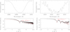 |
Fig. 1. Fourier transforms of primary and secondary lines. Top row: line profiles of the separated spectra of CPD-41° 7742 obtained after application of the brightness ratio for the primary (Si IVλ 4089 line, left panel) and secondary (Si IVλ 4631 line, right panel) stars. Bottom row: Fourier transform of those lines (in black) and best-match rotational profile (in red) for the primary (left panel) and secondary (right panel) stars. |
Best-fit projected rotational velocities as derived from the disentangled spectra of CPD-41° 7742.
3.4. Model atmosphere fitting
The reconstructed spectra of the binary components were analysed by means of the CMFGEN model atmosphere code (Hillier & Miller 1998) to constrain the fundamental properties of the stars. We here refer the reader to Rosu et al. (2022) for information about the code and its limitations.
The CMFGEN spectra were first broadened by the projected rotational velocities determined in Sect. 3.3. We adjusted the stellar and wind parameters following the procedure outlined by Martins (2011).
3.4.1. Primary star
The macroturbulence velocity was adjusted on the wings of the O IIIλ 5592 and Balmer lines, and we derived a value of vmacro = 100 ± 10 km s−1. We adjusted the microturbulence velocity, that is to say, the microturbulence value at the level of the photosphere,  , on the metallic lines and inferred a value of 14 ± 3 km s−1.
The effective temperature was determined by searching for the best overall fit of the He I and He II lines. This was clearly a compromise as we could not find a solution that perfectly fits all helium lines simultaneously. For instance, we found that the strength of the He Iλ 4471 line is underestimated while other He I lines are well-adjusted. Given the luminosity class of the primary, it seems unlikely that this discrepancy reflects the dilution effect discussed by Voels et al. (1989) and Herrero et al. (1992). We discarded some lines that are only weakly sensitive to temperature (He Iλ 4713), or that are blended with neighbouring lines (He Iλ 4026 is blended with the weak but non-zero He IIλ 4026 line and He Iλ 4121 is blended with Si IVλ 4116). Likewise, the He IIλ 5412 line could be impacted by the stellar wind (Herrero et al. 1992). Hence, we adjusted the effective temperature on the He Iλ 4922 line and obtained a value of 31 800 ± 1000 K. With this effective temperature, the He Iλλ 4026, 4713, and 4922 lines as well as the He IIλ 4200 line are well adjusted.
The surface gravity was obtained by adjusting the wings of the Balmer lines Hβ, Hγ, Hδ, H Iλλ 3890, and 3835. We derived log gspectro = 3.76 ± 0.10.
The surface chemical abundances of all elements, including helium, carbon, nitrogen, and oxygen, were set to solar as taken from Asplund et al. (2009). The primary star of CPD-41° 7742 is a typical case where it is impossible to certify whether or not the chemical abundances of the elements differ from solar; the number of parameters we have to adjust exceeds the number of lines we can use for this purpose. For instance, the oxygen abundance could be determined by adjusting the O IIIλ 5592 line as this is the sole oxygen line free of blends. The best fit is obtained for a sub-solar abundance O/H of (4.20 ± 0.20)×10−4. The synthetic CMFGEN spectrum displays a series of weak O III absorption lines (λλ 4368, 4396, 4448, 4454, and 4458) that are not present in the observed spectra (neither before nor after disentangling). These lines are not correctly reproduced by the model, as has been pointed out by several authors (e.g. Raucq et al. 2016; Rosu et al. 2020b, 2022), and hence, are not considered in our analysis. The CMFGEN spectrum also displays the O IIIλ 5508 line, which is not present in the stellar spectrum whereas the O IIλ 4070 line is correctly reproduced. However, this line is blended with C IIIλ 4070 and should therefore be considered with caution. A similar caveat applies to the O IIλ 4185 line that is heavily blended with the C IIIλ 4187 line.
Similarly, the carbon abundance could in principle be adjusted on the C IIIλ 4070 and C IIλ 4267 lines. However, the C IIIλ 4070 line is blended with O IIλ 4070. We note that the C IIIλλ 4647–51 blend and the C IIIλ 5696 line are known to be problematic because their formation processes are controlled by a number of far-UV lines (Martins & Hillier 2012). As a result, the strength and nature of the C IIIλλ 4647–51 blend and of the C IIIλ 5696 line critically depend upon subtle details of the stellar atmosphere model.
Finally, the nitrogen abundance is impossible to determine with accuracy as the N IIIλλ 4510–4540 blend is completely absent from the stellar spectrum, the λλ 4634–4640 complex is heavily blended with Si IV, O II, and C III lines, and the N IIIλ 4379 line is heavily blended with the C IIIλ 4379 line.
Regarding the wind parameters, the clumping parameters were fixed: The volume filling factor f1 was set to 0.1, and the f2 parameter controlling the onset of clumping was set to 100 km s−1. For the sake of completeness, we varied f1 from 0.05 to 0.2 and we did not observe any significant difference as the resulting spectra perfectly overlapped. Likewise, the β parameter of the velocity law was fixed to 1.1 as suggested by Muijres et al. (2012) for an O9.5 V type star. Again for the sake of completeness, we tested a value of 1.0 for β but did not observe any significant differences as the resulting spectra perfectly overlapped.
In principle, the wind terminal velocity could be derived from the Hα line. However, because of the degeneracy between the wind parameters, we decided to fix the value of v∞ to 2380 km s−1 as measured by Sana et al. (2005). Regarding the mass-loss rate, the main diagnostic lines in the optical domain are Hα and He IIλ 4686. We measured a value of Ṁ = (5.0 ± 1.0) × 10−8 M⊙ yr−1 based on the Hα line but could not reproduce the He IIλ 4686 line correctly.
The stellar and wind parameters of the best-fit CMFGEN model atmosphere are summarised in Table 3. The normalised disentangled spectra of the primary of CPD-41° 7742 are illustrated in Fig. 2 along with the best-fit CMFGEN adjustment.
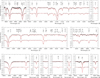 |
Fig. 2. Normalised disentangled spectra (in black) of the primary and secondary stars of CPD-41° 7742 (the spectrum of the secondary star is shifted by +0.3 in the y-axis for clarity) together with the respective best-fit CMFGEN model atmosphere (in red). |
Stellar and wind parameters of the best-fit CMFGEN model atmosphere derived from the separated spectra of CPD-41° 7742.
3.4.2. Secondary star
We proceeded differently for the secondary star. As the O IIIλ 5592 line, the main diagnostic line for the macroturbulence velocity, is not present in the spectrum of the secondary star, we could not adjust vmacro on this line and had to rely on He I and Balmer lines instead. Hence, we adjusted vmacro, the effective temperature, and the surface gravity simultaneously in an iterative manner in order to get the best fit of the spectrum. We derived a value of vmacro = 50 ± 10 km s−1.
The effective temperature was determined based on the sole He I lines, as the secondary spectrum lacks He II lines. As for the primary star, we adjusted the effective temperature mainly on the He Iλ 4922 line, and found a value of 26 000 ± 1000 K. With this effective temperature, the He Iλλ 4471, 4713, and 5016 lines are also well adjusted. However, the He Iλ 4026 line is slightly overestimated while the He Iλλ 4388, 5876, and 7065 lines are slightly underestimated.
The surface gravity was obtained by adjusting the wings of the Balmer lines Hβ, Hγ, Hδ, and H Iλλ 3835, 3890. We derived log gspectro = 4.00 ± 0.10. With this value, the wings of Hβ, Hδ, and H Iλ 3835 are well adjusted while the wings of the two other lines are overestimated.
We adjusted the microturbulence velocity on the metallic lines and obtained 10 ± 3 km s−1 for  . The surface chemical abundances of all elements, including He, C, N, and O were set to solar according to Asplund et al. (2009) for the same reasons as for the primary star.
Regarding the wind parameters, the clumping parameters f1 and f2 were fixed as for the primary star. We fixed the β parameter of the velocity law to 1.1 as we have no indication about the value of this parameter and did not find any significant difference when varying the value of this parameter.
We adjusted a mass-loss rate of Ṁ = (5.0 ± 1.0) × 10−10 M⊙ yr−1 based on the Hγ and Hα lines. The wind terminal velocity was then adjusted based on the strength of the Hα line. We found a value of v∞ = 2040 km s−1.
The stellar and wind parameters of the best-fit CMFGEN model atmosphere are summarised in Table 3. The normalised disentangled spectra of the secondary of CPD-41° 7742 are illustrated in Fig. 2 along with the best-fit CMFGEN adjustment.
4. Radial velocity analysis
The total dataset of RVs consists of our 166 primary and secondary RVs determined via disentangling (see Sect. 3.1) complemented by 37 primary and nine secondary RVs coming from the literature. For the primary star, there are 16 RVs from Hill et al. (1974), four from Levato & Morrell (1983), three from Perry et al. (1990), eight from García & Mermilliod (2001), and six from Sana et al. (2003, their CAT data). The secondary RVs come from García & Mermilliod (2001), three values, and from Sana et al. (2003), six values. As reported by Sana et al. (2003), some of the Julian dates quoted by García & Mermilliod (2001) were wrong by one day. These were corrected and reported by Sana et al. (2003) and we therefore adopted these corrected dates in the present analysis. In total, we ended up with a series of 203 primary RV data points spanning about 49 years and 175 secondary RV data points spanning about 22 years. We adopted the following values for the uncertainties on the primary RVs: 10 km s−1 for the data of Hill et al. (1974), Levato & Morrell (1983), and García & Mermilliod (2001), 15 km s−1 for the data of Perry et al. (1990), and 5 km s−1 for the CAT data of Sana et al. (2003). For the RVs derived from the spectral disentangling, we adopted formal errors of 5 km s−1, as the small errors derived as part of the disentangling method would bias the adjustment given our high number of RVs compared to those coming from the literature. Since the secondary RVs are only available for the most recent data and are subject to larger errors than the primary RVs, we did not use them in the determination of the rate of apsidal motion.
For each time of observation t, we adjusted the primary RV data as in Rosu et al. (2022), explicitly accounting for the apsidal motion through the variation of the argument of periastron of the primary orbit. The systemic velocity γP of each subset of our total dataset was adjusted so as to minimise the sum of the residuals, because RVs of different spectral lines potentially yield slightly different apparent systemic velocities.
To find the values of the six free parameters (the orbital period Porb, the eccentricity e, the time T0 of periastron passage, the argument of periastron of the primary orbit ω0 at epoch T0, the apsidal motion rate  , and the semi-amplitude of the RV curve KP) that provide the best fit to the whole set of primary RV data, we scanned the parameter space in a systematic way. The projections of the 6D parameter space onto the 2D planes are illustrated in Fig. 3. We observe a strong degeneracy between the different parameters of the fit, as shown by the numerous local minima. We are therefore not able to derive a unique solution with sufficient accuracy, at least without the prior knowledge of one of these parameters.
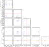 |
Fig. 3. Confidence contours for the best-fit parameters obtained from the adjustment of the primary RV data of CPD-41° 7742. The best-fit solution is shown in each panel by the black filled dot. The corresponding 1σ confidence level is shown by the blue contour. For comparison, the value of the apsidal motion rate (respectively eccentricity) and its error bars as derived in Sect. 6 are shown in orange (respectively pink) respectively by the solid and dashed lines. |
To solve this issue, we fixed the eccentricity and apsidal motion rate to the values of 0.0204 and  yr−1 as derived from the analysis of the times of minima (see Sect. 6), and left the four other parameters free. As Fig. 3 indicates, this value of
  is in agreement with one local minimum of the global adjustment of the RVs. The projections of the 4D parameter space onto the 2D planes are illustrated in Fig. 4. The corresponding orbital parameters are given in Table 4. Figure 5 illustrates the best fit of the RV data at 12 different epochs, where the primary and secondary RV curves are depicted in blue and red, respectively.
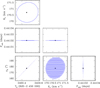 |
Fig. 4. Confidence contours for the best-fit parameters obtained from the adjustment of the primary RV data of CPD-41° 7742 when the eccentricity and the apsidal motion rate are fixed to the values of 0.0204 and |

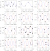 |
Fig. 5. Comparison between the measured RVs of the primary (filled dots) and secondary (open dots, when available) of CPD-41° 7742 with the orbital solution from Table 4. The blue and red lines represent the fitted RV curve of the primary and secondary stars, respectively. Top panels: data from Hill et al. (1974, left), Levato & Morrell (1983, middle), and García & Mermilliod (2001, right). Second row, left panel: yields the CAT/CES data from Sana et al. (2003). All other panels correspond to RVs derived in this paper. |
Best-fit orbital parameters of CPD-41° 7742 obtained from the adjustment of the RV data.
The primary and secondary RVs of an SB2 binary are related to each other through the mass ratio  . We derived a value q = 0.562 ± 0.006 from the RVs coming from the disentangling process, and we used this result to build an SB2 orbital solution for CPD-41° 7742. Our best-fit parameters and their 1σ errors are listed in Table 4, where aP sin i and aS sin i stand for the minimum semi-major axis of the primary and secondary stars, respectively, MPsin3i and MSsin3i stand for the minimum mass of the primary and secondary stars, respectively, and
  is the reduced χ2.
We note that the mass ratio we found is slightly higher than the value of 0.555 ± 0.005 quoted by Sana et al. (2003) from the He I lines but is compatible with this value within the error bars. We further note that our semi-amplitudes of the primary and secondary RV curves are higher than those derived by Sana et al. (2003, see Table 1). These differences are likely due to the two-Gaussian fit used by Sana et al. (2003) to establish their RVs.
5. Photometric analysis
The Nightfall binary star code (version 1.92), developed by R. Wichmann, M. Kuster, and P. Risse2 (Wichmann 2011), was used to analyse the light curves of the binary CPD-41° 7742. The Roche potential, scaled with the instantaneous separation between the stars, is used to describe the stellar shape. We neglected any stellar surface spots. In total, we have eight model parameters: the effective temperatures Teff, P and Teff, S of the primary and secondary stars, the Roche lobe filling factors (ratios between the stellar polar radius and the polar radius of the associated instantaneous Roche lobe at periastron) fP and fS of the primary and secondary stars, the mass ratio q, the orbital eccentricity e, the orbital inclination i, and the argument of periastron ω. As the Bochum and uvby observations are not polluted by the presence of another star in the field, there is no need to include any third light in the model. The TESS observations are, however, polluted by the presence of the massive binary HD 152248 in the field, and hence, a third light contribution is included in the model for these observations. Such a third light contribution leads to further degeneracies among the best-fit solutions of the light curve. Hence, we decided to analyse the TESS data with the stellar parameters set to their values inferred from the fit of the Bochum data.
The period of the system was fixed to the instantaneous sidereal period Pecl, that is to say, the time interval between two primary minima. Its expression as a function of the orbital period, the eccentricity, the apsidal motion rate, and the argument of periastron is given by Eq. (A.24) of Schmitt et al. (2016):
where  is expressed in radians per day. For the value of Porb given in Table 4 and the values of e and
  derived in Sect. 7, Pecl ranges between 2.440609 and 2.440637 d.
The existence of apsidal motion in the system and the different levels of third light contamination of the various datasets prevent us from performing a simultaneous analysis of all photometric data. Hence, we performed the analysis of the four datasets (Bochum 6051 and 4686, uvby, TESS-12, and TESS-39) separately. The dates of primary minima were directly adjusted on the phase-folded light curve. We obtained 2 450 553.544, 2 451 932.48551, 2 458 629.5717, and 2 459 361.7536 HJD for the Bochum, uvby, TESS-12, and TESS-39 photometry, respectively.
The photometric data collected with the Bochum telescope cover an interval of 28 days, which is short enough to neglect any change of ω. We fixed the effective temperatures of the stars to the values derived from the CMFGEN analysis (see Table 3 and Sect. 3.4). We fixed the mass ratio to the value derived from the RV analysis (see Table 4). We were thus left with five parameters to adjust: i, e, fP, fS, and ω. In this way, the best-fit Roche-lobe filling factor of the primary star (near 0.73) was systematically smaller than that of the secondary star (≃0.83), leading to fS/fP = 1.14. With the stellar temperatures fixed to their values derived from the spectroscopic analysis, this result is at odds with the spectroscopic brightness ratio that rather implies RP/RS = 2.05 ± 0.45 and thus fS/fP = 0.63 ± 0.14.
To solve this issue, we explored a grid of models where we varied the value of fP between 0.80 and 0.90 and fixed fS in such a way that the ratio fS/fP is equal to the spectroscopic value or this value ±1σ. These tests indicated that the best-fit solutions were obtained when fS was at the higher end of the ‘authorised’ range and for fP values near 0.81. To account for the fact that the spectroscopic temperatures are subject to some uncertainties, we then started exploring another grid of models for fP between 0.80 and 0.84, but this time leaving fS and the secondary’s effective temperature as free parameters. The main results of this approach are summarised in Table 5. The 1σ and 90% confidence contours in the (fP, e)-plane is shown in Fig. 6 and the best fit are shown in Fig. 7. The eclipse depths of both eclipses of the two Bochum datasets are given in Table 6.
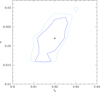 |
Fig. 6. Confidence contours of the best-fit solutions of the Bochum photometry of CPD-41° 7742 in the (fP, e)-plane. The best-fit solution is shown by the black filled dot. The corresponding 1σ and 90% confidence levels are shown by the dark and light blue contours, respectively. |
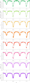 |
Fig. 7. Best-fit solution to the Bochum 6051 and 4686, uvby, TESS-12, and TESS-39 photometric data of CPD-41° 7742. The light curves have been phase-folded using Pecl. The dates of primary minima are 2 450 553.544, 2 451 932.48551, 2 458 629.5717, and 2 459 361.7536 HJD for the Bochum, uvby, TESS-12, and TESS-39 photometry, respectively. |
Best-fit parameters of the Bochum 6051 and 4686 photometric data of CPD-41° 7742.
Time at mid-exposure and depths of the primary and secondary eclipses for the photometric observations of CPD-41° 7742.
Compared to solutions with the secondary effective temperature fixed, the quality of the fits is improved. The secondary star’s best-fit photometric temperature is lower than the spectroscopic value by about 2000 K (i.e. twice the estimated error on the spectroscopic value). Yet, it should be noted that the primary spectroscopic temperature also has an uncertainty of 1000 K, which is not accounted for in the photometric fits. Since the photometric solution is mostly sensitive to the ratio of the temperatures, increasing the primary temperature by 1000 K (i.e. 1σ of the spectroscopic value) actually leads to a secondary effective temperature of 24 960 K, which is at a bit more than 1σ from the spectroscopic value. For consistency, in the following, we adopt an error of 1000 K on the secondary effective temperature. The V-band brightness ratio of the two stars for these solutions amounts to ≃0.20 in excellent agreement with the spectroscopic value. Hence, the issue mentioned above can be solved in this way. The value of 0.0204 for the eccentricity derived from the analysis of the times of minima (see Sect. 6) is fully consistent with the best estimate obtained here.
Finally, we analysed the uvby, TESS-12, and TESS-39 photometry fixing all parameters to their best-fit values (see Table 5) except for e fixed to the value of 0.0204 (see Sect. 6), and for ω that was left as a free parameter. For the uvby photometry, the best fit gives  and is illustrated in Fig. 7. The four light curves are well-adjusted. In order to check if our best-fit solution is robust and not biased by the best-fit solution of the Bochum photometry, we performed three additional adjustments of the uvby photometry: For all three cases, in addition to ω, the secondary effective temperature was left free; for two of these, the secondary Roche lobe filling factor was also left free; and for one of these, the inclination was left as a free parameter too. The results are given in Table 7. The reduced
  decreases slightly as more free parameters are adopted, but the best-fit values of the parameters do not change significantly, which ensures that our best-fit solution with all parameters fixed except for ω is robust. The eclipse depths of both eclipses of the photometric datasets are given in Table 6. Regarding the TESS-12 and TESS-39 data, we also left the third light contribution I3 as a free parameter of the adjustment and obtained
  , I3 = 0.147 ± 0.010, and
  = 694.4, and
  , I3 = 0.071 ± 0.012, and
  = 347.0, respectively. We note that the large values of
  have no physical sense and arise because of the underestimate of the errors on the TESS data. The best fits are shown in Fig. 7. As the eclipses of the TESS light curves are diluted by the residual contamination of third light, we cannot compare their depths to those of the Bochum and uvby photometric data.
Best-fit parameters of the uvby photometry of CPD-41° 7742.
6. Times of minimum
The times of minima of photometric observations can serve for the determination of the apsidal motion rate of an eclipsing binary system (Giménez & Bastero 1995). We computed the phase difference between the primary and secondary eclipses,
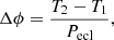
for the different sets of observations. We adjusted a second-order polynomial as well as a Gaussian to the eclipses for the Bochum 6051 and 4686, uvby, TESS-12, and TESS-39 separately, and found the values given in Table 8.
We then computed the phase difference between the times of the secondary and primary eclipses, respectively T2 and T1, following the relation adapted from Giménez & Bastero (1995):

where A1, A3, and A5 are functions of the inclination and the eccentricity given by Eqs. (16), (18), and (20) of Giménez & Bastero (1995). We adjusted this curve to the observations explicitly accounting for the apsidal motion rate  through the variation of ω with time. This is illustrated in Fig. 8. The best-fit adjustment (summarised in Table 9) is obtained for e = 0.0204 ± 0.0016,
 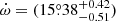 yr−1,
yr−1, 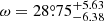 at the time of the Bochum observations, and χν = 0.1539. The projections of the 3D parameter space onto the 2D planes are illustrated in Fig. 9.
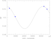 |
Fig. 8. Values of the phase difference Δϕ between the primary and secondary eclipses as a function of time inferred from the times of minima of the light curves. The blue symbols correspond to the data of the fits of the Bochum 6051 and 4686, uvby, TESS-12, and TESS-39 photometry. The solid line corresponds to our best-fit value of Δϕ from Eq. (3). |
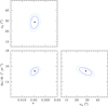 |
Fig. 9. Confidence contours for the best fit obtained from the adjustment of the phase differences between the times of the secondary and primary eclipses using Eq. (3). The best-fit solution is shown in each panel by the black filled dot. The corresponding 1σ and 99% confidence levels are shown by the dark and light blue contours, respectively. |
Best-fit parameters of the adjustment of the phase difference between the primary and secondary eclipses for the photometric observations of CPD-41° 7742.
7. CPD-41° 7742 orbital and physical parameters
The best-fit parameters obtained from the adjustment of the RVs (see Table 4), the Bochum light curves (see Table 5), and the adjustment of the times of minima (see Table 9) are combined to finally establish the orbital and physical parameters of CPD-41° 7742. A semi-major axis of 23.09 ± 0.16 R⊙ is deduced for the system. Absolute masses for the primary and secondary stars MP = 17.8 ± 0.5 M⊙ and MS = 10.0 ± 0.3 M⊙, as well as absolute radii for the primary and secondary stars RP = 7.57 ± 0.09 R⊙ and 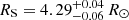 are derived. This leads to photometric values of the surface gravities of the primary and secondary stars log gP = 3.93 ± 0.02 and log gS = 4.17 ± 0.02. From the photometric stellar radii, the primary effective temperature derived in Sect. 3.4, and the secondary effective temperature derived in Sect. 5, we inferred bolometric luminosities
 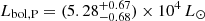 and
and 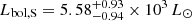 for the primary and secondary stars, respectively. If we further assume the stellar rotational axes to be aligned with the normal to the orbital plane, the combination of the orbital inclination, the stellar radii, and the projected rotational velocities of the stars derived in Sect. 3.3 yields rotational periods for the primary and secondary stars Prot, P = 2.71 ± 0.14 days and Prot, S = 2.42 ± 0.19 days. The ratio between rotational angular velocity and instantaneous orbital angular velocity at periastron amounts to 0.86 ± 0.04 and 0.97 ± 0.08 for the primary and secondary stars, respectively. Pseudo-synchronisation is achieved for the secondary star and about to be achieved for the primary star.
The apsidal motion rate of a binary system is the sum of a Newtonian contribution,  , and a general relativity correction,
  . We refer to Rosu et al. (2022) for a review of the useful equations. The Newtonian contribution and the general relativistic correction amount to
  yr−1 and
  yr−1, respectively, in the case of CPD-41° 7742. We refer to Rosu et al. (2022) for a review of the useful equations. The Newtonian contribution depends upon the internal mass distribution of the stars through the internal structure constants k2 of the stars:
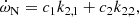
where c1 and c2 are two functions of stellar and orbital parameters (Rosu et al. 2022). We define a weighted-average mean of the internal structure constants,
the value of which amounts to  in the present case. As the secondary star is smaller and less massive than the primary star, its k2-value exceeds that of the primary. Therefore, we have
  . Observationally, we have
  and
and 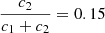 , meaning that the k2, 1 has a much higher weight in the calculation of
  .
.
8. Stellar structure and evolution models
We computed stellar evolution models with the Code Liégeois d’Évolution Stellaire3 (Clés,Scuflaire et al. 2008, see also Rosu et al. 2022 for an overview of the main features of Clés and its minimisation routine min-Clés used in the present context). The aim of the present analysis is to see whether standard models reproducing the stellar physical properties are also capable of reproducing the apsidal motion rate inferred in Sect. 6. For all models built, we adopted the mass-loss rate scaling factor ξ = 1.
In a first attempt to obtain stellar evolution models representative of both stars, we built two Clés models (Models IP and IS) simultaneously, adopting the six corresponding constraints (M, R, and Teff of both stars), and leaving the initial masses of the two stars and the age of the binary system as the only three free parameters. For both stars, we adopted an overshooting parameter αov = 0.20, and no turbulent diffusion. The parameters of the best-fit models are reported in Table 10. Except for the secondary effective temperature, all stellar parameters are well-reproduced within their error bars. The age of the binary system is estimated at 6.25 ± 0.30 Myr while the total (Newtonian + general relativistic) apsidal motion rate is estimated at  yr−1, slightly larger than the observational value (see Sect. 6). We then computed two models independently for each star (Models IIP and IIS) adopting the same constraints and free parameters. The best-fit models in this case (see Table 10) have ages of 6.13 ± 0.37 and 7.47 ± 1.30 Myr. The physical parameters of the two stars are better reproduced but the apsidal motion rate, of
  yr−1, is still slightly larger than the observational value. We note that in principle, we should compute the apsidal motion rate of the system based on two stellar models having the same age. Nonetheless, the independent primary and secondary models have ages compatible within their error bars.
In a last attempt to reproduce the stellar properties and the apsidal motion rate of the system, we built a series of five independent models (Models III (1) to (5)) for the two stars adopting the same constraints as before, an overshooting parameter of 0.20, 0.25, 0.30, 0.35, and 0.40, respectively, and, as free parameters, the age, the initial mass, and the turbulent diffusion. The best-fit models are reported in Table 10. The models perfectly reproduce the stellar properties of the primary star thanks to the addition of turbulent diffusion. The best-fit turbulent diffusion coefficient decreases with increasing overshooting, indicating that both effects affect the k2 parameter in a similar way (see also the discussion in Rosu et al. 2020a). We note that the turbulent diffusion of the secondary models converge towards a value of 0 cm2 s−1. This behaviour has already been observed for the binary system HD 152219 and we refer to the discussion in Rosu et al. (2022). The age estimates range from 6.78 to 6.83 Myr for the primary star and from 6.99 to 7.88 Myr for the secondary star. For each series of models, we computed the apsidal motion rate of the binary system and obtained values ranging between  and
and  yr−1. These values are compatible within the error bars with the observational value. We therefore conclude that to reproduce the apsidal motion rate of the binary system, and hence, the internal structure of the stars composing the system, turbulent diffusion needs to be included inside the models, at least for the most massive star of the system. These results confirm those obtained by Rosu et al. (2020a) for the twin system HD 152248, and Rosu et al. (2022) for HD 152219, two systems located in the same cluster NGC 6231.
9. Revisiting HD 152218
In this section, we briefly reconsider the eccentric massive binary HD 152218, also located in NGC 6231. Since our previous work on this system (Rauw et al. 2016), TESS photometry has become available and the min-Clés routine allows for a more efficient search for best-fit stellar evolution models, which now also includes turbulent diffusion. The stellar and orbital parameters of HD 152218 (taken from the RV analysis of Rauw et al. 2016) are summarised in Table 11. We determined a Newtonian and a general relativistic contributions to the apsidal motion rate of  yr−1 and
  yr−1, respectively.
Observational properties of the binary system HD 152218 taken from Rauw et al. (2016).
9.1. Analysis of TESS data
HD 152218 was observed by TESS during the same sectors as CPD-41° 7742 (i.e. sectors 12 and 39). We performed an extraction of the light curves with a 30 and 10 min cadences again for TESS-12 and TESS-39, respectively. For this purpose, we used the Lightkurve software and followed the reduction steps explained in Sect. 2.2. We adopted here the pca-5 for the background subtraction. This results in a total of 1257 and 3705 data points for TESS-12 and TESS-39, respectively.
We analysed the light curves of HD 152218 with the Nightfall code. We fixed the effective temperatures, the eccentricity, and the orbital period to the values quoted by Rauw et al. (2016, see Table 11). The only free parameters were the orbital inclination, the longitude of periastron, and the Roche lobe filling factors of the two stars. The best-fit adjustments are given in Table 12 (we note again that the large values of  have no physical sense and arise because of the underestimate of the errors on the TESS data) and illustrated in Fig. 10.
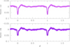 |
Fig. 10. Best-fit solution to the TESS-12 and TESS-39 photometry of HD 152218. The light curves have been phase-folded with Pecl = 5.60415 d computed using Eq. (1). |
Best-fit parameters of the TESS photometry of HD 152218.
The values for the longitude of periastron expected at the times of the TESS-12 and TESS-39 observations from the apsidal motion rate derived from the RV analysis of Rauw et al. (2016) amount to  and
and  , respectively. Whilst the value of ω inferred for the TESS-12 light curve is compatible within the error bars, this is not the case for the value of omega inferred for the TESS-39 light curve. In addition, the value of ω should be larger for the TESS-39 light curve than for the TESS-12 one, as omega increases with time.
In the case of HD 152218, the fact that there is a single eclipse leads to a degeneracy between the primary and secondary Roche lobe filling factors, and the orbital inclination that can shift the formally best-fit solution to values of the Roche lobe filling factors that are inconsistent with the spectroscopic brightness ratio. To overcome this difficulty, we scanned the parameter space fixing i, fP, and fS to the values that, considering Fig. 6 of Rauw et al. (2016), give a brightness ratio in accordance with the spectroscopic value and are acceptable (at 1σ) with the ASAS-3 photometry. In this way, ω was the only free parameter of the adjustment. The combination of parameters that give acceptable results in terms of  give ω values ranging from
  to
to  for the TESS-12 data and from
  to
to  for the TESS-39 data. These values are in agreement, within the error bars, with those expected from the spectroscopic apsidal motion rate. These solutions all predict an inclination between 67° and 69°.
We therefore conclude that the previously reported apsidal motion rate derived by Rauw et al. (2016) is confirmed by the new photometric data.
9.2. Stellar evolution models
We built stellar evolution models with the min-Clés routine for HD 152218, adopting as constraints the masses, radii, and effective temperatures of the stars. We fixed ξ = 1, and left the age, initial masses, and turbulent diffusion as free parameters.
We first built two models (Models IP and IS) simultaneously for the two stars. The parameters of the best fit are reported in Table 13. Except for the radius of the secondary star, all stellar parameters are well-reproduced within their error bars. The age of the binary system is estimated at 5.79 Myr, confirming the value obtained by Rauw et al. (2016). The apsidal motion rate is estimated at  yr−1. This value is slightly lower than the observational value.
To solve the discrepancies in the secondary radius and in the apsidal motion rate, we further built a series of five independent models (Models IIP (1) to (5) and IIS (1) to (5)) for the two stars adopting an overshooting parameter of 0.20, 0.25, 0.30, 0.35, and 0.40, respectively. The best-fit models are reported in Table 13. They reproduce well the stellar properties of both stars. As for the primary star of CPD-41° 7742, we observe that the amount of turbulent diffusion necessary to fit the stellar properties decreases with the increasing overshooting parameter. The age estimates range from 6.71 to 6.76 Myr for the primary star and from 11.59 to 11.67 Myr for the secondary star. Given the important age difference between the primary and secondary models, we cannot compute a coherent apsidal motion rate for the binary system by simply summing the contributions of the two stars taken at different ages.
As discussed in Rauw et al. (2016), the presence of only one eclipse in the light curves of HD 152218 leads to degeneracies in the determination of the stellar radii, the ratio of effective temperatures, and the inclination of the system. Rauw et al. (2016) derived a ratio of 1.18 ± 0.20 between the primary and secondary radii based on their ratio of bolometric luminosities and effective temperatures. Assuming that the radius of the primary star is well constrained, this relation translates into a secondary radius of 7.12 R⊙. Thus, we built a series of five models for the secondary star assuming a constraint on the stellar radius of 7.12 rather than 7.80 R⊙. These best-fit models (Models IIIS (1) to (5)), which reproduce well the stellar properties, are reported in Table 13. Compared to Models IIS, the age estimate is lower and closer to that of the primary star models, and the apsidal motion rate, computed based on Models IIP and IIIS, amounts to  yr−1 to
  yr−1.
yr−1.
We then built a Clés evolutionary sequence for the secondary star, starting with an initial mass of 15.17 M⊙ and having αov = 0.20 and no turbulent diffusion. We stopped the sequence at the age of the best-fit models of the primary star (Models IIP) and obtained a model of mass 15.11 M⊙, radius 6.39 R⊙, effective temperature 29 674 K, and k2, 2 = 7.68 × 10⁻³. Combined with Model IIP (1) for the primary star, we obtained an apsidal motion rate of  yr−1. This value is slightly lower than the observational value but agrees with the previously obtained value.
Finally, in a last attempt to reproduce the apsidal motion rate of the system, we built models for the two stars assuming DT = 0 cm2 s−1 (Models IVP for the primary star, Models IVS and VS for the secondary star, when the constraint on the radius is 7.80 and 7.12 R⊙, respectively). The stellar properties are still well reproduced within the error bars, and the apsidal motion rate (neglecting the age difference between the primary and secondary models) amounts to  yr−1 to
  yr−1 and
  yr−1 to
  yr−1 when Models IVS and VS are considered. This value is compatible within the error bars with the observational value. Initial masses of 20.6 ± 1.5 and 15.5 ± 1.1 M⊙ are derived for the primary and secondary stars, respectively, and the binary’s age is estimated at 5.2 ± 0.8 Myr as derived from the primary models.
10. Conclusion
The eccentric massive binary CPD-41° 7742, belonging to the open cluster NGC 6231, has been analysed both from an observational and a stellar evolution point of views. The spectroscopic observations were used to obtain the reconstructed spectra of the components together with their RVs at each time of observation. Combined with the RVs coming from the literature, the latter were subsequently used to determine stellar and orbital parameters for the system. We further analysed the photometric observations of the system to constrain the inclination of the orbit as well as the absolute masses and radii of the stars. We solved the inconsistency highlighted by Sana et al. (2005) and Bouzid et al. (2005) between the longitude of periastron inferred by the RV analysis on the one hand and the photometric analysis on the other hand by analysing the phase differences between the times of secondary and primary minima of the eclipses for the different sets of photometric observations explicitly accounting for the apsidal motion. In this way, we obtained a rate of apsidal motion of  yr−1. We then computed stellar evolution models for the two stars. The best-fit models of the stars, in terms of the masses, radii, and effective temperatures, predict a theoretical apsidal motion rate compatible within the error bars with the observed one provided that turbulent mixing is introduced in the primary stellar evolution models, therefore confirming the results obtained for the twin system HD 152248 by Rosu et al. (2020a) and for HD 152219 by Rosu et al. (2022). The binary’s age is estimated at 6.8 ± 1.4 Myr and initial masses of 18.0 ± 0.5 and 9.9 ± 0.3 M⊙ are derived for the primary and secondary stars, respectively.
The eccentric massive binary HD 152218, belonging to the same cluster, was reconsidered in light of the newly available TESS data and the updated Clés code. The results of the light curve analysis are coherent with those obtained from our previous study (Rauw et al. 2016). The stellar evolution models reproduce the observational properties of the stars within their error bars, including the apsidal motion rate, and predict initial masses of 20.6 ± 1.5 and 15.5 ± 1.1 M⊙ for the primary and secondary stars, respectively, as well as a binary age of 5.2 ± 0.8 Myr.
In total, we have analysed four massive eccentric binary systems belonging to the NGC 6231 cluster in a series of papers (see Rosu et al. 2020a,b, 2022) and the present work. The ages estimated for these systems point towards an age estimate for the massive star population of the cluster of 5 to 9.5 Myr. This value is compatible with the ages estimated (between 1 and 7 Myr with a small peak at 3 Myr) based on the low-mass pre-main-sequence stars of the cluster, though pointing towards the upper allowed range of values. The large scatter is partially due to the observational uncertainties (e.g. the lack of the secondary eclipse in HD 152218 induces degeneracies in the determination of the stellar parameters) as well as due to physical assumption lying behind the stellar evolution models. These studies confirm the need for enhanced mixing inside the stellar evolution models to reproduce the observational stellar properties. They suggest that massive stars have larger convective cores than usually considered in stellar evolution codes.
The code is available at: https://www.physik.uni-hamburg.de/en/hs/group-schmidt/members/wichmann-rainer/nightfall.html
Acknowledgments
S.R., Y.N., and E.G. acknowledge support from the Fonds de la Recherche Scientifique (F.R.S.-FNRS, Belgium). We thank Drs John Hillier and Rainer Wichmann for making their codes, respectively CMFGEN and Nightfall, publicly available. We thank Dr Martin Farnir for the development of the min-Clés routine and his help regarding its use. The authors thank the referee for his/her suggestions and comments towards the improvement of the manuscript.
References
- Asplund, M., Grevesse, N., Sauval, A. J., & Scott, P. 2009, ARA&A, 47, 481 [NASA ADS] [CrossRef] [Google Scholar]
- Bailer-Jones, C. A. L., Rybizki, J., Fouesneau, M., Demleitner, G., & Andrae, R. 2021, AJ, 161, 147 [NASA ADS] [CrossRef] [Google Scholar]
- Baroch, D., Giménez, A., Ribas, I., et al. 2021, A&A, 649, A64 [NASA ADS] [CrossRef] [EDP Sciences] [Google Scholar]
- Bouzid, M. Y., Sterken, C., & Pribulla, T. 2005, A&A, 437, 769 [NASA ADS] [CrossRef] [EDP Sciences] [Google Scholar]
- Claret, A. 1999, A&A, 350, 56 [NASA ADS] [Google Scholar]
- Claret, A., & Torres, G. 2019, ApJ, 876, 134 [Google Scholar]
- Claret, A., Giménez, A., Baroch, A., et al. 2021, A&A, 654, A17 [NASA ADS] [CrossRef] [EDP Sciences] [Google Scholar]
- Conti, P. S., & Alschuler, W. R. 1971, ApJ, 170, 325 [NASA ADS] [CrossRef] [Google Scholar]
- Gaia Collaboration (Brown, A. G. A., et al.) 2021, A&A, 649, A1 [NASA ADS] [CrossRef] [EDP Sciences] [Google Scholar]
- García, B., & Mermilliod, J.-C. 2001, A&A, 368, 122 [NASA ADS] [CrossRef] [EDP Sciences] [Google Scholar]
- Giménez, A., & Bastero, M. 1995, Ap&SS, 226, 99 [Google Scholar]
- González, J. F., & Levato, H. 2006, A&A, 448, 283 [NASA ADS] [CrossRef] [EDP Sciences] [Google Scholar]
- Gray, D. F. 2008, The Observation and Analysis of Stellar Photospheres, 3rd edn. (Cambridge: Cambridge University Press) [Google Scholar]
- Gray, R. O. 2009, A Digital Spectral Classification Atlas, https://ned.ipac.caltech.edu/level5/Gray/frames.html [Google Scholar]
- Herrero, A., Kudritzki, R. P., Vilchez, J. M., et al. 1992, A&A, 261, 209 [NASA ADS] [Google Scholar]
- Hill, G., Crawford, D. L., & Barnes, J. V. 1974, AJ, 79, 1271 [Google Scholar]
- Hillier, D. J., & Miller, D. L. 1998, ApJ, 496, 407 [NASA ADS] [CrossRef] [Google Scholar]
- Humphreys, R. M., & McElroy, D. B. 1984, AJ, 284, 565 [NASA ADS] [CrossRef] [Google Scholar]
- Kaufer, A., Stahl, O., Tubbesing, S., et al. 1999, The Messenger, 85, 8 [NASA ADS] [Google Scholar]
- Kuhn, M. A., Getman, K. V., Feigelson, E. D., et al. 2017, AJ, 154, 214 [NASA ADS] [CrossRef] [Google Scholar]
- Levato, H., & Malaroda, S. 1980, PASP, 92, 323 [NASA ADS] [CrossRef] [Google Scholar]
- Levato, H., & Morrell, N. 1983, Astrophys. Lett., 23, 183 [NASA ADS] [Google Scholar]
- Mahy, L., Gosset, E., Sana, H., et al. 2012, A&A, 540, A97 [NASA ADS] [CrossRef] [EDP Sciences] [Google Scholar]
- Martins, F. 2011, Bull. Soc. R. Sci. Liège, 80, 29 [NASA ADS] [Google Scholar]
- Martins, F., & Hillier, D. J. 2012, A&A, 545, A95 [NASA ADS] [CrossRef] [EDP Sciences] [Google Scholar]
- Martins, F., & Plez, B. 2006, A&A, 457, 637 [NASA ADS] [CrossRef] [EDP Sciences] [Google Scholar]
- Mathys, G. 1988, A&AS, 76, 427 [NASA ADS] [Google Scholar]
- Mayor, M., Pepe, F., Queloz, D., et al. 2003, The Messenger, 114, 20 [NASA ADS] [Google Scholar]
- Muijres, L. E., Vink, J. S., de Koter, A., Müller, P. E., & Langer, N. 2012, A&A, 537, A37 [NASA ADS] [CrossRef] [EDP Sciences] [Google Scholar]
- Pasquini, L., Avila, G., Blecha, A., et al. 2002, The Messenger, 110, 1 [Google Scholar]
- Perry, C. L., Hill, G., Younger, P. F., & Barnes, J. V. 1990, A&AS, 86, 415 [NASA ADS] [Google Scholar]
- Raucq, F., Rauw, G., Gosset, E., et al. 2016, A&A, 588, A10 [NASA ADS] [CrossRef] [EDP Sciences] [Google Scholar]
- Rauw, G., Rosu, S., Noels, A., et al. 2016, A&A, 594, A33 [NASA ADS] [CrossRef] [EDP Sciences] [Google Scholar]
- Ricker, G. R., Winn, J. N., Vanderspek, R., et al. 2015, J. Astron. Telesc. Instrum. Syst., 1, 014003 [Google Scholar]
- Rosu, S., Noels, A., Dupret, M.-A., et al. 2020a, A&A, 642, A221 [NASA ADS] [CrossRef] [EDP Sciences] [Google Scholar]
- Rosu, S., Rauw, G., Conroy, K. E., et al. 2020b, A&A, 635, A145 [NASA ADS] [CrossRef] [EDP Sciences] [Google Scholar]
- Rosu, S., Rauw, G., Farnir, M., Dupret, M.-A., & Noels, A. 2022, A&A, 660, A120 [NASA ADS] [CrossRef] [EDP Sciences] [Google Scholar]
- Royer, P., Vreux, J.-M., & Manfroid, J. 1998, A&AS, 130, 407 [NASA ADS] [CrossRef] [EDP Sciences] [Google Scholar]
- Sana, H., Hensberge, H., Rauw, G., & Gosset, E. 2003, A&A, 405, 1063 [NASA ADS] [CrossRef] [EDP Sciences] [Google Scholar]
- Sana, H., Antokhina, E., Royer, P., et al. 2005, A&A, 441, 213 [NASA ADS] [CrossRef] [EDP Sciences] [Google Scholar]
- Sana, H., Rauw, G., Sung, H., Gosset, E., & Vreux, J.-M. 2007, MNRAS, 377, 945 [NASA ADS] [CrossRef] [Google Scholar]
- Sana, H., Gosset, E., Nazé, Y., Rauw, G., & Linder, N. 2008, MNRAS, 386, 447 [Google Scholar]
- Schmitt, J. H. M. M., Schröder, K.-P., Rauw, G., et al. 2016, A&A, 586, A104 [NASA ADS] [CrossRef] [EDP Sciences] [Google Scholar]
- Scuflaire, R., Théado, S., Montalbán, J., et al. 2008, Ap&SS, 316, 83 [Google Scholar]
- Simón-Díaz, S., & Herrero, A. 2007, A&A, 468, 1063 [NASA ADS] [CrossRef] [EDP Sciences] [Google Scholar]
- Slettebak, A., Collins, G. W., Boyce, P. B., White, N. M., & Parkinson, T. D. 1975, ApJS, 29, 137 [NASA ADS] [CrossRef] [Google Scholar]
- Sota, A., Maíz Apellániz, J., Walborn, N. R., et al. 2011, ApJS, 193, 24 [Google Scholar]
- Sota, A., Maíz Apellániz, J., Morrell, N. I., et al. 2014, ApJS, 211, 10 [Google Scholar]
- Sterken, C. 1983, The ESO Messenger, 33, 10 [NASA ADS] [Google Scholar]
- Sterken, C. 1994, in The Impact of Long-Term Monitoring on Variable-Star Research, NATO ARW, eds. C. Sterken, & M. de Groot (Kluwer Academic Publishers), NATO ASI Ser. C, 436, 1 [NASA ADS] [Google Scholar]
- Struve, O. 1944, ApJ, 100, 189 [Google Scholar]
- Sung, H., Bessel, M. S., & Lee, S.-W. 1998, AJ, 115, 734 [NASA ADS] [CrossRef] [Google Scholar]
- Sung, H., Sana, H., & Bessell, M. S. 2013, AJ, 145, 37 [NASA ADS] [CrossRef] [Google Scholar]
- Torres, G., Andersen, J., & Giménez, A. 2010, A&ARv, 18, 67 [Google Scholar]
- Voels, S. A., Bohannan, B., Abbott, D. C., & Hummer, D. G. 1989, ApJ, 340, 1073 [NASA ADS] [CrossRef] [Google Scholar]
- Walborn, N. R., & Fitzpatrick, E. L. 1990, PASP, 102, 379 [Google Scholar]
- Wichmann, R. 2011, Astrophysics Source Code Library [record ascl:1106.016] [Google Scholar]
- Zacharias, N., Finch, C. T., Girard, T. M., et al. 2013, AJ, 145, 44 [Google Scholar]
Appendix A: Journal of the spectroscopic observations of CPD-41° 7742
This appendix provides the journal of the spectroscopic observations of CPD-41° 7742 (Table A.1).
Journal of the spectroscopic observations of CPD-41° 7742.
All Tables
Best-fit projected rotational velocities as derived from the disentangled spectra of CPD-41° 7742.
Stellar and wind parameters of the best-fit CMFGEN model atmosphere derived from the separated spectra of CPD-41° 7742.
Best-fit orbital parameters of CPD-41° 7742 obtained from the adjustment of the RV data.
Best-fit parameters of the Bochum 6051 and 4686 photometric data of CPD-41° 7742.
Time at mid-exposure and depths of the primary and secondary eclipses for the photometric observations of CPD-41° 7742.
Best-fit parameters of the adjustment of the phase difference between the primary and secondary eclipses for the photometric observations of CPD-41° 7742.
Observational properties of the binary system HD 152218 taken from Rauw et al. (2016).
All Figures
|
Fig. 1. Fourier transforms of primary and secondary lines. Top row: line profiles of the separated spectra of CPD-41° 7742 obtained after application of the brightness ratio for the primary (Si IVλ 4089 line, left panel) and secondary (Si IVλ 4631 line, right panel) stars. Bottom row: Fourier transform of those lines (in black) and best-match rotational profile (in red) for the primary (left panel) and secondary (right panel) stars. |
| In the text | |
|
Fig. 2. Normalised disentangled spectra (in black) of the primary and secondary stars of CPD-41° 7742 (the spectrum of the secondary star is shifted by +0.3 in the y-axis for clarity) together with the respective best-fit CMFGEN model atmosphere (in red). |
| In the text | |
|
Fig. 3. Confidence contours for the best-fit parameters obtained from the adjustment of the primary RV data of CPD-41° 7742. The best-fit solution is shown in each panel by the black filled dot. The corresponding 1σ confidence level is shown by the blue contour. For comparison, the value of the apsidal motion rate (respectively eccentricity) and its error bars as derived in Sect. 6 are shown in orange (respectively pink) respectively by the solid and dashed lines. |
| In the text | |
|
Fig. 4. Confidence contours for the best-fit parameters obtained from the adjustment of the primary RV data of CPD-41° 7742 when the eccentricity and the apsidal motion rate are fixed to the values of 0.0204 and |
| In the text | |
|
Fig. 5. Comparison between the measured RVs of the primary (filled dots) and secondary (open dots, when available) of CPD-41° 7742 with the orbital solution from Table 4. The blue and red lines represent the fitted RV curve of the primary and secondary stars, respectively. Top panels: data from Hill et al. (1974, left), Levato & Morrell (1983, middle), and García & Mermilliod (2001, right). Second row, left panel: yields the CAT/CES data from Sana et al. (2003). All other panels correspond to RVs derived in this paper. |
| In the text | |
|
Fig. 6. Confidence contours of the best-fit solutions of the Bochum photometry of CPD-41° 7742 in the (fP, e)-plane. The best-fit solution is shown by the black filled dot. The corresponding 1σ and 90% confidence levels are shown by the dark and light blue contours, respectively. |
| In the text | |
|
Fig. 7. Best-fit solution to the Bochum 6051 and 4686, uvby, TESS-12, and TESS-39 photometric data of CPD-41° 7742. The light curves have been phase-folded using Pecl. The dates of primary minima are 2 450 553.544, 2 451 932.48551, 2 458 629.5717, and 2 459 361.7536 HJD for the Bochum, uvby, TESS-12, and TESS-39 photometry, respectively. |
| In the text | |
|
Fig. 8. Values of the phase difference Δϕ between the primary and secondary eclipses as a function of time inferred from the times of minima of the light curves. The blue symbols correspond to the data of the fits of the Bochum 6051 and 4686, uvby, TESS-12, and TESS-39 photometry. The solid line corresponds to our best-fit value of Δϕ from Eq. (3). |
| In the text | |
|
Fig. 9. Confidence contours for the best fit obtained from the adjustment of the phase differences between the times of the secondary and primary eclipses using Eq. (3). The best-fit solution is shown in each panel by the black filled dot. The corresponding 1σ and 99% confidence levels are shown by the dark and light blue contours, respectively. |
| In the text | |
|
Fig. 10. Best-fit solution to the TESS-12 and TESS-39 photometry of HD 152218. The light curves have been phase-folded with Pecl = 5.60415 d computed using Eq. (1). |
| In the text | |
Current usage metrics show cumulative count of Article Views (full-text article views including HTML views, PDF and ePub downloads, according to the available data) and Abstracts Views on Vision4Press platform.
Data correspond to usage on the plateform after 2015. The current usage metrics is available 48-96 hours after online publication and is updated daily on week days.
Initial download of the metrics may take a while.