| Issue |
A&A
Volume 664, August 2022
|
|
|---|---|---|
| Article Number | A45 | |
| Number of page(s) | 14 | |
| Section | Stellar structure and evolution | |
| DOI | https://doi.org/10.1051/0004-6361/202243595 | |
| Published online | 03 August 2022 | |
Characterisation of Galactic carbon stars and related stars from Gaia EDR3⋆
1
Dpto. Física Teórica y del Cosmos, Universidad de Granada, 18071 Granada, Spain
e-mail: This email address is being protected from spambots. You need JavaScript enabled to view it.
2
Université Côte d’Azur, Observatoire de la Côte d’Azur, CNRS, Laboratoire Lagrange, Nice, France
3
Institut de Ciències del Cosmos, Universitat de Barcelona (IEEC-UB), Martí i Franquès 1, 08028 Barcelona, Spain
Received:
21
March
2022
Accepted:
25
May
2022
Abstract
The third early Gaia data release (EDR3) has improved the accuracy of the astrometric parameters of numerous long-period variable (LPV) stars. Many of these stars are on the asymptotic giant branch (AGB), showing either a C-rich or O-rich envelope and are characterised by high luminosity, changing surface composition, and intense mass loss. This make them very useful for stellar studies. In a previous investigation, we used Gaia DR2 astrometry to derive the luminosity function, kinematic properties, and stellar population membership of a flux-limited sample of carbon stars in the solar neighbourhood of different spectral types. Here, we extend this initial study to more recent surveys with a greater number of Galactic carbon stars and related stars by adopting the more accurate EDR3 astrometry measurements. Based on a much larger statistics, we confirm that N- and SC-type carbon stars share a very similar luminosity function, while the luminosities of J-type stars (Mbol) are fainter by half a magnitude on average. R-hot type carbon stars have luminosities throughout the RGB, which favours the hypothesis of an external origin for their carbon enhancement. Moreover, the kinematic properties of a significant fraction of the R-hot stars are compatible with the thick-disc population, in contrast with that of N- and SC-type stars, which would belong mostly to the thin disk. We also derive the luminosity function of a large number of Galactic extrinsic and intrinsic (O-rich) S stars and show that the luminosities of the latter are typically higher than the predicted onset of the third dredge-up during the AGB for solar metallicity. This result is consistent with these stars being genuine thermally pulsing AGB stars. On the other hand, using the so-called Gaia-2MASS diagram, we show that the overwhelming majority of the carbon stars identified in the LAMOST survey as AGB stars are probably R-hot and/or CH-type stars. Finally, we report the identification of ∼2660 new carbon stars candidates that we identified through their 2MASS photometry, their Gaia astrometry, and their location in the Gaia-2MASS diagram.
Key words: stars: late-type / stars: carbon / techniques: miscellaneous
The Gaia-EDR3 identification number of these stars together with the full version of Table 1 are only available at the CDS via anonymous ftp to cdsarc.u-strasbg.fr (130.79.128.5) or via http://cdsarc.u-strasbg.fr/viz-bin/cat/J/A+A/664/A45
© C. Abia et al. 2022
 Open Access article, published by EDP Sciences, under the terms of the Creative Commons Attribution License (https://creativecommons.org/licenses/by/4.0), which permits unrestricted use, distribution, and reproduction in any medium, provided the original work is properly cited.
This article is published in open access under the Subscribe-to-Open model. This email address is being protected from spambots. You need JavaScript enabled to view it. to support open access publication.
1. Introduction
In a previous study (Abia et al. 2020, hereafter Paper I), a sample of 210 carbon stars of N-, SC-, J- and R-hot spectral types was selected in the solar vicinity, mainly based on the flux-limited sample of carbon stars by Claussen et al. (1987). The main aim of the project is to fully characterise the properties of these stars in terms of luminosity, kinematics, and chemical composition to distinguish their evolutionary status and typical stellar masses and to define to which Galactic population they belong. Although the chemical properties of each of these carbon star types are relatively well known (Wallerstein & Knapp 1998; Abia et al. 2003; Habing & Olofsson 2004; Zamora et al. 2009, and references therein; see also Paper I), the conclusions deduced from these abundance studies are frequently limited by the uncertain determination of the luminosity and kinematic properties of these stars. The Gaia all-sky survey has changed this situation by providing astrometric data with an unprecedented accuracy of all Galactic stellar populations (Gaia Collaboration 2018), in particular of long period variables (LPV; Mowlavi et al. 2018), among which most of these carbon star types are found.
In Paper I, we used Gaia DR2 astrometric measurements to derive the luminosities and kinematic properties of already well-known red giant carbon stars of different spectral types located in the solar vicinity. We found that the luminosity function (LF) of N- and SC-type stars is quite similar, but is clearly different from that of J-type stars. Interestingly, we also found extended tails to low and high luminosity in the LF of the N-type stars and discussed the implications that this may have for the theoretical lower and upper mass limits for the formation of intrinsic AGB carbon stars. On the other hand, the derived LF of R-hot stars revealed that these stars should be in the RGB phase rather than in the red clump of the HB, as previously suggested (Bergeat et al. 2002). However, these findings were based on a small statistics, in particular for SC-type (10 objects), J-type (21 objects), and R-hot stars (35 objects).
In the present study, we extend our previous analysis to more than 2000 objects that we extracted from different recent giant stars surveys. All the different spectral types of carbon stars mentioned above were considered, and we adopted the more accurate Gaia EDR3 astrometric data (Lindegren et al. 2021). Our present analysis also includes the identification of a large number of new AGB carbon star candidates in the 2MASS survey (Skrutskie et al. 2006) through the use of the Gaia-2MASS diagram (Lebzelter et al. 2018). The sample is introduced in Sect. 2, and the analysis is carried out in Sects. 3 and 4. In Sect. 5 we explore the capability of the Gaia-2MASS diagram to identify the different spectral types of AGB stars, and we present the catalogue of new carbon star candidates in Sect. 6. A summary of the main results of this study is made in Sect. 7.
2. Star sample and Galactic distribution
We extended the sample of carbon stars studied in Paper I by including the collected Galactic infrared carbon stars (IRCSs) in Chen & Yang (2012), the new catalogue of carbon stars from the LAMOST DR2 survey (Ji et al. 2016), and the list of J-type Galactic carbon stars in Chen et al. (2007). We recall that the carbon stars studied in Paper I were taken from the flux-limited sample of Galactic carbon stars studied by Claussen et al. (1987), which includes about 215 carbon stars of N-, J-, and SC-types (see Paper I for details of the selection).
The sample of Chen & Yang (2012) collects all of the IRCSs from the literature (Chan & Kwok 1990; Groenewegen et al. 2002; Chen & Chen 2003; Gupta et al. 2004; Le Bertre et al. 2005) and some known carbon stars with SiC emission at 11.2 μm that were not listed previously. In total, the sample includes 974 objects, most of them quoted as being carbon stars according to the SIMBAD1 database. Nevertheless, a significant number of objects in the Chen & Yang (2012) sample have no spectral type identification and appear in SIMBAD just as possible carbon stars (see below). The LAMOST survey includes 894 carbon stars that were identified by several spectral line indices from low-resolution spectra. By combining several CN and C2 bands, Ji et al. (2016) identified carbon stars of N-, CH-, and R-hot types, although several dozen objects were also quoted as of possible N-type or of unknown carbon type. Below, we show that most of these objects with dubious spectral classification in the LAMOST sample are probably not genuine AGB carbon stars. On the other hand, the infrared study by Chen et al. (2007) included 113 Galactic stars of J type. A few of them were included in the sample of J-type stars we studied in Paper I. Finally, for comparison purposes, we completed our stellar sample with the Galactic S-type stars studied by Chen et al. (2019): 151 extrinsic, and 190 intrinsic. We recall that intrinsic S-type stars are O-rich objects (C/O < 1) that follow the M-S-C sequence evolution in the AGB phase. They show intense Tc lines and s-element enhancements in their spectra (Van Eck et al. 1998; Van Eck & Jorissen 1999; Uttenthaler & Lebzelter 2010; Uttenthaler 2013). The detection of the unstable element technetium in the spectra of these stars is an evidence of the in situ operation of the s-process nucleosynthesis (see e.g. Straniero et al. 2006; Karakas & Lattanzio 2014). Extrinsic S-type stars are also O-rich objects in a binary system with a white dwarf (WD, undetected) and also have enhanced s-process elements at the stellar surface, but as the result of mass transfer from a former AGB star (now the WD) to a less evolved companion (now the S-type star). They do not show intense Tc lines in their optical spectra.
Next, we cross-match the stars of the Chen et al. (2007), Chen & Yang (2012), and Ji et al. (2016) samples with the stars studied in Paper I to avoid repetitions. We found 82 objects in common with Paper I that are distributed among all spectral types of the carbon stars. These stars were removed from the surveys mentioned above, and this was then our initial sample of stars. In contrast to the stars studied in Paper I, there is not information in the literature about the detailed chemical composition for the overwhelming majority of the new carbon stars included here. However, considering their position in the Galactic plane and their kinematics (see below and Sect. 4), most of them belong to the Galactic thin-disc population. We thus may guess that their metallicity is close to solar. Therefore and unless explicitly mentioned, we assume solar metallicity for all of the stars in our sample throughout this paper. This does not apply to the CH-type stars in the LAMOST sample; most of these stars are known to be metal-poor objects (see e.g. Wallerstein & Knapp 1998). Finally, we filtered this sample according to the accuracy of their EDR3 parallaxes and the corresponding derived distances as described below.
To recover the most accurate distances of these stars, we first selected those with Gaia parallaxes that were derived from five-parameter astrometric solutions with a renormalised unit weight error, RUWE, smaller than 1.4. We then selected those whose astrometric fidelity factor for their astrometric solution exceeded 0.5, according to Rybizki et al. (2022). This factor allows identifying possible spurious parallaxes and the best Gaia astrometric solutions. For the selected stars, we then adopted the photo-geometric distances from Bailer-Jones et al. (2021). Then, we again filtered the sample and chose only stars with a Gaia EDR3 parallax uncertainty ≤10%. This condition ensures that the distance adopted from Bailer-Jones et al. (2021) is close to the inverse of the parallax, and therefore has little dependence on the adopted prior. In Paper I we discussed that large colour variations (most of our stars are variables of different variability types) may not significantly affect the parallax measurements. We refer to the discussion there for details. Figure 1 compares the histogram of the Gaia DR3 parallaxes in the original sample of stars with that deduced from the Bailer-Jones et al. (2021) photo-geometric distances adopted in this study after applying our parallax quality criteria. These criteria include the use of positive parallaxes alone. The bin size in the histograms is 0.1 mas, which is the typical uncertainty in the parallax (∼10%) for most of the stars in the final sample. The stars that did not fulfil our parallax criteria are clearly removed in the full parallax range. As a consequence, the final sample should not contain any bias on the distances of the stars.
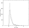 |
Fig. 1. Comparison of the histogram of the Gaia DR3 parallaxes in the initial sample of stars (dashed line) with the parallaxes deduced from the Bailer-Jones et al. (2021) distances adopted after filtering the sample according to our quality parallax criteria (continuous line). The bin size is 0.1 mas (see text). |
We compared the distances obtained for the stars in common with Paper I with those derived here. We find an excellent agreement: a mean difference of −34 ± 190 pc in the sense DR2 minus EDR3 distances. Only for two N-type stars, IRC +60393 and V497 Pup, is the difference significant, which is due to the ∼50% higher parallax in Gaia DR2 for these stars. For three stars (V437 Aql, RU Vir, HIP 44812, and HIP 66317), we find differences of ∼20% in the parallax DR2-EDR3. On the other hand, we also found a moderate change in the EDR3 Gaia photometry values (GBP and GRP) for the stars V Cyg and TX Psc with respect to those in DR2. This will imply a significant change in their position in the Gaia-2MASS diagram (see below). In Paper I we have reported that TX Psc was suspected to be a binary star and that it was the brightest N-type star in our sample (G = 3.72 mag according to DR2). This bright G-magnitude may be affected by saturation problems that could occur for the brightest Gaia DR2 targets and might also affect the determination of the parallax. In EDR3, the estimated uncertainty in the G, GBP, and GRP magnitudes has been considerably reduced for this star.
After the quality parallax and distance filters described above, our final sample contains 491 carbon stars of N type, 22 of SC type, 83 of J type, 234 of R-hot type, and 276 of CH type. For the spectral types N, SC, J, and R-hot, this represents an increase of more than a factor of two in the number of objects with respect to Paper I. To these, we added 107 extrinsic and 91 intrinsic S stars of Ji et al. (2016). The total is then 1304 objects whose luminosity function and Galactic location and kinematics we studied. However, some stars that fulfilled our parallax and distance filters were still excluded from the luminosity function analysis because of their uncertain classification type and bolometric correction: 192 objects labelled extreme infrared, and 37 objects as possible carbon stars in the Chen & Yang (2012) sample, and 86 and 69 objects labelled possible carbon stars and of unknown type, respectively, in the LAMOST sample (see below). There are 1688 objects in total.
The stars we selected are listed in Table 1. We preferentially adopted their variable star designation (from Samus & Durlevich 2004) or, when this was not available, their IRAS name (Neugebauer et al. 1984), their name in the LAMOST catalogue (Zhao et al. 2012), or the name that is used most frequently in the literature according to the SIMBAD database. Table 1 also reports their Gaia-EDR3 identification (Col. 2), the distance estimation (Col. 8), and the infrared 2MASS photometry (J, Ks) (Cols. 6 and 7) corrected for Galactic extinction (Cols. 3–5; see below). According to the 2MASS survey, the average uncertainty in the J and Ks magnitudes in our stellar sample is 0.05 ± 0.12 and 0.07 ± 0.20 mag, respectively. Many of the objects studied here lack an accurate or individual determination of the radial velocity. For the sake of homogeneity, we therefore adopted the values given in Gaia DR2 (Katz et al. 2019) as the velocity along the line of sight (Vrad) even though the Gaia/RVS spectral domain is not optimal for deriving Vrad in cool carbon-rich stars. Nevertheless, for the stars in Paper I for which more accurate Vrad values in the literature were found, we confirmed that the Gaia DR2 values do not significantly differ from those adopted in Paper I.
Derived data for the sample stars.
Figures 2–4 show the location of the sample stars in the X − Y coordinates around the Sun and above and below the Galactic plane (see also Table 1) for the stars in Chen et al. (2007) and Chen & Yang (2012) (Fig. 2), stars in the LAMOST sample (Fig. 3), and the S-type stars in Chen et al. (2019) (Fig. 4). Their Cartesian coordinates were directly derived from the Gaia EDR3 sky coordinates and adopted distances. Median uncertainties are ±12, ±16, ±13, and ±13 pc for X, Y, Z and R, respectively (see Paper I for details of the derivation of the uncertainties).
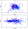 |
Fig. 2. Top: location of the stellar sample of carbon stars around the Sun. The Sun is placed at (X, Y) = (0, 0). Stars are taken from the surveys by Chen et al. (2007) and Chen & Yang (2012). Blue dots show normal N-type carbon stars; red dots represent J-type stars, and cyan dots show stars of unknown type according to Chen & Yang (2012) that are labelled possible carbon stars in SIMBAD. Bottom: distribution above or below the Galactic plane vs. galactocentric distance. The Sun is at R = 8.34 kpc. The typical uncertainty in the (X, Y, Z) coordinates is ±20 pc, and it is ±50 pc for the galactocentric distance (see text). |
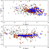 |
Fig. 3. Same as Fig. 2 for the carbon stars in the LAMOST survey (Ji et al. 2016). Solid blue dots show N-type carbon stars, grey dots represent CH-type stars, and brown dots show R-hot stars. The limits of the X- and Y-axes and R coordinates are different from Fig. 2. |
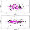 |
Fig. 4. Same as Fig. 2 for the S stars in Chen et al. (2019). Solid black circles show extrinsic stars, and purple circles show intrinsic stars. The limits of the X- and Y-axes and R coordinates are different from Fig. 2. |
The top panels in Figs. 2 and 4 show that the spatial distribution of the stars in Chen et al. (2007, 2019) and Chen & Yang (2012) are fairly uniform around the Sun, although the stars labelled possible carbon stars seem to be located at Y < 0 values and very close the Galactic plane (cyan circles in Fig. 2).
When we consider only the carbon stars of N type in this study and those in Paper I (491 stars in total), a crude fit to the |Z|-coordinate distribution with an exponential function results in a scale height of zo ∼ 220 pc (see Fig. 5, top panel), which agrees with the value obtained in Paper I within the uncertainty. We do not show in this plot the |Z|-distribution for SC-type stars because there are so few of them. However, a similar fit is compatible with a scale height identical to that of N-type stars. Only ∼6% stars of this type (see the bottom panel in Fig. 2) have |Z|> 0.5 kpc. This scale-height can be used to estimate the typical mass of carbon star progenitors by using tabulations for the scale heights of main-sequence stars as a function of spectral class (e.g. Miller & Scalo 1979). This shows that stars with a mean scale height in the range 160−200 pc have a mass between 1.5 and 1.8 M⊙. These values are fully consistent with theoretical determinations of the typical mass for an AGB carbon star (see e.g. Straniero et al. 2006; Karakas & Lattanzio 2014). In the same way, while the estimated scale height for intrinsic S stars is quite similar to that of N-type stars (zo ∼ 210 pc; see Figs. 4 and 5), extrinsic S stars and J-type stars (Fig. 5) have higher zo values: 280 and 300 pc, respectively. Because the scale height of the Galactic stellar population is thought to be a function of age (mass) (see e.g. Dove & Thronson 1993), this implies that these two types of stars are likely older and typically have lower masses than the N-type stars. This disagrees for J-type stars with our conclusion in Paper I, where we found a similar scale height for J- and N-type stars. Our previous conclusion was biased by the low number of J-type stars in the sample. J-type stars not only differ in chemical composition (see Paper I) and luminosity (see below) with respect to normal N-type stars, but additionally have a different Galactic distribution. This might indicate that they are a completely different population of stars compared to the N-type stars. On the other hand, based on intrinsic S stars with a very similar scale height as N-type stars, we may conclude that the former are the progenitors of the normal AGB carbon stars, as expected on theoretical grounds.
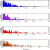 |
Fig. 5. Histograms showing the distribution (normalised to the maximum number of stars) of the |Z|-coordinate for the different spectral types. From top to bottom: normal N-type carbon stars (blue), extrinsic (black) and intrinsic (purple) S stars, J-type stars (red), and R-type stars (brown). The X-axis for the R-type stars is different. For N-type normal carbon stars, orange lines show exponential fits to the distribution with scale heights zo = 260, 220, and 180 pc from top to bottom. Similar fits give an estimate of the scale-height for the other spectral types (see text). The bin size is 20 pc. |
The stars in the LAMOST sample that are classified as N type have an identical distribution above and below the Galactic plane (see Fig. 3, bottom panel) as those in Fig. 2. However, we show below that many of these stars are too faint to be in the AGB phase. Figure 3 also shows that many R-hot carbon stars and the overwhelming majority of CH-type stars are located at large distances above (below) the Galactic plane; the average values are 1.2 ± 1.5 kpc, and 2.7 ± 2.5 kpc, respectively. This is confirmed by the |Z|-distribution of the R-type stars (Fig. 5, bottom panel). An exponential fit to this distribution gives a scale height of zo ∼ 1.3 kpc. This confirms the conclusion that was reached in previous studies (Wallerstein & Knapp 1998; Knapp et al. 2001; Izzard et al. 2007, 2008; Zamora et al. 2009) that these types of carbon stars mainly belong to the Galactic thick-disc population and would also have lower masses than N-type stars.
3. Luminosities
We retrieved the 2MASS J and K photometry (Cutri et al. 2003) from the SIMBAD database and corrected them for interstellar extinction using the Bailer-Jones et al. (2021) distances and the Gaia Galactic coordinates. We followed the same method as in Paper I to derive the luminosities of the stars. We adopted the empirical BCK versus (J − K) relation for carbon stars obtained by Kerschbaum et al. (2010), which is based on a critical revision of previous studies of bolometric corrections for cool giants. For (J − K) between 1.0 to 4.4 mag, the maximum standard deviation of this relation is 0.11 mag, although for values (J − K)≥2.2 mag the scatter increases up to 0.15 mag. For very red objects, in particular for many IRAS sources in the Chen & Yang (2012) sample, we therefore instead used the empirical BCK versus K − [12.5] relation from Guandalini et al. (2006) when the [12.5] colour was available in the literature; otherwise, the particular object was rejected from the analysis. For for the O-rich S stars in the present study, we also adopted the BCK versus (J − K) relation derived by Kerschbaum et al. (2010) for M stars (see Paper I for details).
In Paper I we used the Galactic extinction model by Arenou et al. (1992). In this study, however, we wished to test the sensitivity of the derived luminosities on the extinction model by using other more recent Galactic extinction models: the Bayestar19 model based on the E(B − V) colour excess (Green et al. 2019), which was also used in the Gaia EDR3 collaboration (Gaia Collaboration 2021); the Gaia-2MASS 3D Galactic maps by Lallement et al. (2019), and the Galactic model by Drimmel et al. (2003). For the reddening corrections, we used the relations AK = 0.114AV and AJ = 2.47AK, except when we used the Green et al. (2019) model, in which case we used the corrections given in Gaia Collaboration (2021) study (see Table B.1). The 3D dust-reddening maps from Bayestar19 (Green et al. 2019) are based on Gaia DR2 parallaxes and stellar photometry from Pan-STARRS 1 and 2MASS. This map covers the sky north of a declination of −30° out to a distance of a few kiloparsec. The spatial limitation means that between 10% and 30% of the sample stars do not fall within the selected sky coverage. The 3D absorption map from Drimmel et al. (2003) provides the V-band absorption using scaling factors up to 10 kpc. Absorptions towards the inner disc are known to be overestimated, however. Gaia DR2 photometric data were combined with 2MASS measurements to derive extinction in Lallement et al. (2019) up to 3 kpc. We used Lallement et al. (2019) in combination with Marshall et al. (2006) in the outer disc. A correction in the latter was applied to allow a smooth transition. This combination was applied in the last version of Gaia Object Generator (Luri et al. 2014) and published in the Gaia archive. Differences in the AV values estimated from the Arenou et al. (1992) Galactic model and those from Green et al. (2019), Lallement et al. (2019), and Drimmel et al. (2003) models for the stars in common with Paper I are not very significant. For the Kso magnitude, we found a mean difference of −0.02 ± 0.08, −0.03 ± 0.06, and 0.04 ± 0.10 mag in the sense Arenou et al. (1992) minus Green et al. (2019), Lallement et al. (2019) and Drimmel et al. (2003) magnitudes, respectively, while for the Jo magnitude, the differences are −0.046 ± 0.2, −0.085 ± 0.15, and −0.12 ± 0.23 mag, respectively. We do not find any correlation of these differences with the distance of the object. We note that most of the dispersion found in these differences is produced by a small number of stars for which there is a large discrepancy in the AV value estimated according to Arenou et al. (1992) and the three alternative Galactic extinction models used here.
Figure 6 shows the comparison between the AV values derived from the Lallement et al. (2019) model and those from the Green et al. (2019) and Drimmel et al. (2003) models for the full sample of stars in this study. The extinction values derived from Lallement et al. (2019) and Drimmel et al. (2003) agree fairly well for AV ≲ 1.7 mag; the mean differences are 0.00 ± 0.40 mag in the sense Lallement et al. (2019) minus Drimmel et al. (2003). For higher values, AV ≳ 1.7 mag, there is a significant discrepancy between the two models, although this affects a limited number of objects in our sample. Sources with AV ≳ 1.7 mag have heliocentric distances larger than ∼2 − 3 kpc, precisely where Marshall et al. (2006) overtakes the new estimates by Lallement et al. (2019) and, as shown by Marshall et al. (2006), the differences with Drimmel et al. (2003) are as expected. The comparison with Green et al. (2019) (bottom panel in Fig. 6) reveals the same pattern: a mean difference of −0.20 ± 0.40 mag for AV ≲ 1.7 mag, while for larger AV, Lallement et al. (2019) obtained systematically higher values, but again this affects a limited number of objects. We note that the overwhelming majority of the objects for which large differences in AV are found are located at very low Galactic latitude and at heliocentric distances larger than 2.5 kpc. This distance approximately coincides with the transition to the outer disc where Lallement et al. (2019) combines with the Marshall et al. (2006) extinction values. In any case, although the choice of the extinction model may produce significant differences in the luminosity estimation for some particular objects, we confirmed that the global luminosity functions (see below) are not significantly affected. The luminosity function is obtained from the Ks magnitude, which is only slightly affected by Galactic extinction. For this reason, we finally decided to use the interstellar extinctions obtained from Lallement et al. (2019) (in combination with Marshall et al. (2006)) that allowed an estimate of AV for 100% of the stars in the final sample, while ∼95% and ∼70% can be determined in the cases of the Drimmel et al. (2003) and Green et al. (2019) models, respectively. Unfortunately, the Lallement et al. (2019) model does not estimate the uncertainty in AV for individual objects.
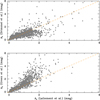 |
Fig. 6. Comparison of the interstellar extinction AV derived from the different Galactic extinction models used in this study. The dashed orange line shows the 1:1 relation. |
The extinction corrected J and Ks magnitudes are given in Table 1 for all the sample stars. MKs and Mbol magnitudes were then derived from the distance modulus relation. Uncertainties in MKs and Mbol are dominated by those in the distances. For the typical parallax uncertainty in our stars (≤10%, see Sect. 2), an error of ∼ ± 0.20 mag in the absolute magnitudes is estimated. Adding the uncertainties associated with the J and Ks magnitudes and the bolometric correction, we estimated ±0.25 mag as a typical error for MKs and Mbol in the full sample of stars. The actual uncertainty is probably slightly higher because we did not consider the uncertainty in AV in this estimate (see above). The corresponding bolometric luminosity distributions and luminosity functions (LF) obtained for all the giant carbon star types in our sample are shown in Fig. 7. We note that to construct the final LF for normal N-type stars (blue histogram, top panel in Fig. 7), we excluded the stars that were classified as of unknown type (36 objects) by Chen & Yang (2012), even though they are quoted as possible carbon stars in the SIMBAD database. Indeed, ∼30% of these objects are classified as RCrB type stars, and another ∼10% as binary or multiple stellar systems in SIMBAD. The R Coronae Borealis (RCrB) stars are rare hydrogen-deficient carbon-rich supergiants that are best known for their spectacular declines in brightness at irregular intervals. Two evolutionary scenarios have been suggested to produce an RCrB star: a double-degenerate merger of two white dwarfs, or a final helium shell flash in a planetary nebula central star (see e.g. Clayton 2012). Furthermore, we also excluded the extreme red objects ((J − Ks)≥2.2 mag, 191 objects) in the sample of Chen & Yang (2012) because BCK is uncertain for these stars. These stars, moreover, may have relatively high mass-loss rates (see below), and the resulting circumstellar extinction causes them to appear fainter in the Ks band. We thus derived the luminosity of 300 of the initial 491 candidate normal AGB carbon stars. From Fig. 7 we see that:
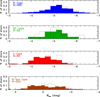 |
Fig. 7. Luminosity distributions (coloured histograms) derived in this study for the different spectral types of Galactic carbon stars (CH-type stars are not shown). The bin size is 0.25 mag. The range in luminosity is different for the R-hot stars that are fainter. For comparison, the corresponding histogram obtained in Paper I for each spectral type is shown in each panel (dotted histograms). |
(a) The average luminosity of N-type stars is ⟨Mbol⟩= − 5.04 ± 0.55 mag. This almost matches the average value obtained in Paper I. For comparison, we show in Fig. 7 (dotted lines) the corresponding LF obtained in Paper I for each spectral type. For N-type stars, the new LF appears to be more symmetric around the average value: a Kolmogorov–Smirnov test confirms that the distribution is consistent with a Gaussian distribution with a p = 0.75. It also shows much less relevant tails at low and mainly at high luminosities. We discuss the significance of these LF tails below. On the other hand, the derived average absolute K magnitude is ⟨MKs⟩= − 8.16 ± 0.57 mag, which is identical to the value derived in Paper I and agrees with the values found in near-IR photographic surveys of the Magellanic Clouds (e.g. Frogel et al. 1980) and the Galaxy (Schechter et al. 1987). As commented in Paper I, the dispersion in MKs is compatible with the typical range in Teff (2500−3500 K) deduced for N-type stars (e.g. Bergeat et al. 2001).
In Paper I we compared (see Fig. 5 and Sect. 3.1 there) the derived LF for N-type stars with the most recent theoretical predictions of the C-rich phase on the AGB (see e.g. Cristallo et al. 2015). A good agreement was found between the observed and predicted LF. However, we remarked then that the existence of two extended tails at high and low luminosity would contradict standard modelling of the AGB phase, in particular, with the lower and upper limit of mass to which a star can become C-rich during the AGB phase (∼1.5 M⊙ and ∼3 M⊙, respectively). The new LF derived here (see Fig. 4, top panel), based on a better statistics and more accurate distances, shows less extended and significant tails (in particular for highest luminosities), which alleviates this contradiction. In any case, we demonstrated in Paper I that the low-luminosity tail might theoretically be accounted for if a small fraction of the N-type stars were extrinsic (binary) stars (an idea first suggested by Izzard & Tout 2004), while the high-luminosity tail would be more difficult to reproduce. Stancliffe et al. (2005) showed that using a high mass-loss prescription during the AGB, the carbon star phase can be more easily attained for the most massive models, those populating the high-luminosity tails of the LF. Nevertheless, the observed existence of N-type stars with Mbol ≲ −5.5 mag, which we confirm here, severely constrains the occurrence of the hot bottom burning (HBB) in intermediate-mass AGB stars. Although intermediate-mass models show that the HBB ceases when the envelope mass is reduced to ∼1 M⊙ (see e.g. Karakas & Lattanzio 2014), the duration of the C-star phase would be too short to provide any sizeable contribution to the LF, but very bright C-stars indeed exist in the LMC with Mbol ∼ −6.8 mag (van Loon et al. 1999; Trams et al. 1999).
(b) The larger number of SC-type stars we analysed here with respect to Paper I allows us to confirm that their LF function is very similar to that of the N-type stars. Moreover, the very similar chemical composition shared by N- and SC-type carbon stars (Abia & Wallerstein 1998; Abia et al. 2002, 2019), as well as their similar location above and below the Galactic plane (see Sect. 2), supports the conclusion that both types of carbon stars originate from similar progenitors. This is compatible with the hypothesis that the SC-type represents a short transition phase (C/O ≈ 1) in between the O-rich (C/O < 1) and the C-rich (C/O > 1) AGB phase. The average luminosity values are ⟨Mbol⟩= − 4.90 ± 0.46 mag and ⟨MKs⟩= − 8.00 ± 0.44 mag.
(c) The new LF for J-type stars is about 0.2 mag dimmer on average compared to that derived in Paper I. We ascribe this difference to the larger statistic used here. Now it is clear that the LF for J-type stars is dimmer than that of N-type carbon stars by ∼0.5 mag. Their average luminosities are ⟨Mbol⟩= − 4.42 ± 0.53 mag, and ⟨MKs⟩= − 7.53 ± 0.57 mag. However, although these luminosites are within the range expected during the AGB phase, a non-negligible fraction of the J-type stars is fainter than Mbol ∼ −4.0 mag, which represents the threshold for the occurrence of third dredge-up (TDU) episodes (see e.g. Straniero et al. 2003; Cristallo et al. 2011). Therefore, we confirm our conclusion of Paper I that the origin of J-type stars (as their carbon enhancement) is different from that of N-type stars.
(d) For R-hot carbon stars, we find average values of ⟨Mbol⟩ = 0.05 ± 1.10 mag and ⟨MKs⟩= − 2.47 ± 1.20 mag, which is slightly dimmer than those found in Paper I, but agrees well within the uncertainties. This clearly discards the suggestion that the bulk population of these objects consists of He-burning red clump stars (Knapp et al. 2001) because the luminosity of the red clump for solar metallicity stars is expected at ⟨MKs⟩∼ − 1.6 ± 0.3 mag (e.g. Alves 2000; Castellani et al. 2000; Salaris & Girardi 2002). The derived luminosities place the R-hot stars throughout the RGB phase. When we assume a typical mass of ∼1.0 M⊙ and Z ∼ Z⊙ stellar models, the bulk of the observed R-hot stars would instead have luminosities that are typical of the RGB bump and would vary from the luminosity of the first dredge-up almost to the luminosity of the RGB tip. This wide luminosity range is difficult to associate with internal processes of mixing that are able to enrich the envelope in carbon during the RGB. Therefore, the hypothesis of an extrinsic origin (or triggered by a merger) of the carbon enhancement in these stars seems to be reinforced. We note, nevertheless, that there is no observational evidence of binarity in these stars (McClure 1984).
Finally, Fig. 8 shows the LF derived for the extrinsic (black) and intrinsic (purple) S stars from the Chen et al. (2019) survey. To our knowledge, this LF is derived in such a large number of S stars for the first time. The average luminosities are ⟨Mbol⟩= − 4.42 ± 0.68 mag, ⟨MKs⟩= − 7.50 ± 0.79 mag, and ⟨Mbol⟩= − 3.52 ± 0.68 mag, ⟨MKs⟩= − 6.40 ± 0.75 mag for intrinsic and extrinsic S stars, respectively. It is evident that intrinsic S stars have higher luminosities than the extrinsic ones and, in particular, the luminosities of the overwhelming majority are higher than the predicted onset of the TDU during the AGB. For solar metallicity stars, this luminosity limit is Mbol ∼ −4.0 mag, which corresponds to stars with an initial mass above 1.3 M⊙ (see e.g. Siess et al. 2000; Cristallo et al. 2011; Karakas & Lattanzio 2014; Escorza et al. 2017). This result is consistent with intrinsic (Tc-rich) S stars being TP-AGB stars, which agrees with the conclusion recently reached by Shetye et al. (2021), who derived the luminosities of a few S stars from theoretical fits to the spectral energy distributions. Moreover, we also found a considerable number of high-luminosity (Mbol ≤ −5.5 mag) intrinsic S stars (see Fig. 8). This high luminosity is compatible with these stars having M > 3 − 4 M⊙. Stars with such a high mass may experience HBB, which prevents them from becoming C-rich AGB stars. On the other hand, the derived LF of extrinsic S stars (peaking at Mbol ∼ −3.0 mag) is compatible with these objects (binaries) being 1 − 2 M⊙ stars in the RGB phase (Van Eck et al. 1998; Shetye et al. 2018). The high-luminosity (Mbol ≤ −4.0 mag) tail in the LF of extrinsic S stars (see Fig. 8) may correspond to barium stars with masses in excess of ∼2.5 M⊙ that can turn into extrinsic S stars on the early AGB, but they are expected to be rare (see Shetye et al. 2018).
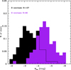 |
Fig. 8. Luminosity distributions derived for the S stars of this study. Purple shows intrinsic S stars, and black shows extrinsic S stars. The bin at Mbol ∼ −2.0 mag. corresponds to the star Hen 4−16 alone, which is quoted in SIMBAD as a possible S star. The bin size is 0.25 mag. |
4. Kinematics
Gaia EDR3 astrometric data provide an additional and valuable piece of information to fully characterise the stellar population of the different carbon star types. As done in Paper I, we computed the galactocentric positions and velocities of our sample stars using the line-of-sight distance estimates of Bailer-Jones et al. (2021), together with the RA, Dec, and proper motions of Gaia EDR3 and our adopted line-of-sight velocities (Vrad, see Sect. 2). Furthermore, we assumed the following parameters: (R⊙, Z⊙) = (8.34, 0.025) kpc (Reid & Honma 2014), (U⊙, V⊙, and W⊙) = (11.1, 12.24, and 7.25) km s−1 (Schönrich 2012), and VLSR = 240 km s−1 (Reid & Honma 2014). For details of the estimation of the uncertainties on each of the derived parameters, we refer to Paper I. The final computed velocity components, Z coordinate, and galactocentric positions of the stars are reported in Table 1.
Figures 9–11 show the Toomre diagrams for the different spectral type stars in this study. For clarity, we separated the sample stars into three different plots, corresponding to the AGB carbon stars (Fig. 9), S-type stars (Fig. 10), and CH-type and R-hot stars (Fig. 11). We excluded from these diagrams the stars listed as possible carbon stars in Chen & Yang (2012), and of possible N-type and as unknown carbon type in Ji et al. (2016). Following the method outlined in Paper I, we computed the likelihood to belong to each of the Galactic components for each star. If this likelihood was greater than 80%, we assigned the membership of the ith component that scored this probability for this star. According to this criterion, stars are listed with a 0, 1, and 2 in Table 1 depending on whether they belong to the thin or thick disc and halo, respectively. Stars labelled with a blank in this table have ambiguous membership according to our criterion. Stars belonging to the thin disc are plotted with solid circles; thick disc with crosses; halo with solid triangles, and open circles represent stars with ambiguous membership.
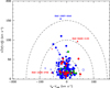 |
Fig. 9. Toomre diagram for the selected carbon stars of this study. The colour symbols are the same as in Fig. 1. Stars are plotted according to their membership probability (> 80%) to belong to the thin disc (solid circles), thick disc (crosses), or halo (triangles) stellar population. Open circles show stars with ambiguous membership (see text). Dashed lines indicate |

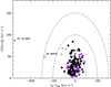 |
Fig. 10. Same as Fig. 9 for extrinsic (black) and intrinsic (purple) S stars. The star HD 160379 (open circle) has an ambiguous Galactic membership population between thick disc and halo according to our criteria (see text). |
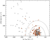 |
Fig. 11. Same as Fig. 9 for the CH-type stars in the LAMOST sample (Ji et al. 2016) together with the R-hot stars also in LAMOST and those included in Paper I (grey and brown symbols, respectively). A significant number of stars classified in LAMOST as R-hot type have ambiguous Galactic population membership (open brown circles), mainly between the thin and thick disc (see text). |
We confirm the figure found in Paper I in the sense that N-, SC-, and J-type carbon stars mostly belong to the thin disc, with a probability rate of 97%, 100% and 90%, respectively. A few N-type stars have typical thick-disc kinematics, and the star IRAS 12227−5045 probably belongs to the halo. This star, together with V CrB and RU Vir identified in Paper I, probably is one of the very few halo AGB carbon stars known in our Galaxy. They deserve high-resolution spectroscopic studies to define their detailed chemical composition. The same remark may be applied to two J-type stars with a probable halo membership: IRAS 14006−5759 and IRAS 09482−5123 (see Fig. 9).
On the other hand, Fig. 10 also shows that the overwhelming majority of extrinsic and intrinsic S stars belong to the Galactic thin-disc population (probability rates of 94% and 96%, respectively). A few extrinsic S stars belong to the thick disc, and we identify the star CD −54 9245 as a possible halo star. We point out that Vanture et al. (2007) did not detect Tc or Li lines in this S star.
Finally, Fig. 11 shows the Toomre diagram for the CH- and R-hot types (the latter type also includes those studied in Paper I). As expected, a significant fraction (∼56%) of the CH-type stars belong to the halo and/or thick-disc population, but a significant number (∼44%) belongs to the thin disc. About 15% of the R-hot stars belong to the thick disc, and two of them (HIP 40374 and J230231.75+210129.7) exhibit kinematics that are fully compatible with the halo. The kinematics of at least 20 additional R-hot stars (open brown circles in Fig. 11, see also Table 1) are compatible with the thick disc, and the rest (∼50%) exhibit thin-disc kinematics. Because the Vz velocity component increases with the stellar age (e.g. Nordström et al. 2004), this figure reinforces our conclusion of Paper I: a significant fraction of the R-hot stars belongs to an older (probably less massive) stellar population than the other types of giant carbon stars. Figure 11 also clearly shows that CH- and R-hot types share rather similar Galactic kinematics. In the next section, we show that they also have very similar luminosities (MKs). The conclusion is tempting that there is a link between these two types of carbon-rich stars. However, most of the CH-type stars are metal-poor binary objects showing s-elements enhancements in their surface, but none of these properties are observed in R-hot stars (Zamora et al. 2009).
5. Identification of the stellar types in the Gaia-2MASS diagram
After we calculated the luminosities of the stars, we constructed the Gaia-2MASS diagram (see Figs. 12 and 13). This was originally designed by Lebzelter et al. (2018) and is especially suitable to highlight the presence of AGB stars. In this diagram, the MKs magnitude is correlated with a particular combination of Gaia and 2MASS photometry through the quantity WRP, BP − RP − WKs, J − Ks, where WRP, BP − RP and WKs, J − Ks are reddening-free Wesenheit functions (Soszyński et al. 2005), defined as WRP, BP − RP = GRP − 1.3(GBP − GRP) and WKs, J − Ks = Ks − 0.686(J − Ks), respectively. In Paper I we demonstrated that this diagram is a powerful tool for analysing and identifying the different spectral types of the AGB stars as a function of chemical type and initial mass.
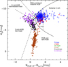 |
Fig. 12. Gaia-2MASS diagram for our main star sample. The curved line delineates the theoretical limit between O-rich (left of the line) and C-rich AGB stars (right of the line). Dashed lines separate sub-groups of stars as indicated in the figure. The colour code for the different AGB types is shown in the bottom right corner. Open blue circles show N-type stars for clarity. Several SC-type stars (green circles) and J-type stars (red circles) are placed in the C-rich zone, but cannot be distinguished in the figure because of crowding. The uncertainty in MKs typically is ±0.23 mag. |
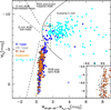 |
Fig. 13. Same as Fig. 12 for the carbon stars in the LAMOST sample by Ji et al. (2016). Grey circles show CH-type stars, brown circles show R-hot stars, blue circles show normal N-type stars, open blue circles show possible N-type stars, and open orange circles show carbon stars of unknown type. For completeness, we show (cyan circles) the carbon stars in Chen & Yang (2012) with (J − Ks) > 2.5 mag. The inset shows a zoom of a small area in the location of the R-hot and CH-type stars (see text). |
Figure 12 shows that the C- and O-rich AGB stars in our study populate different regions, which allows us to easily identify them as long as their distances are known. This diagram also permits the distinction between regions with low-mass, intermediate-mass, and massive O-rich AGB stars, RGB, or faint AGB stars as well as supergiants and extreme C-rich AGB stars, the specific stellar mass range in each of these groups depending on the stellar metallicity (see Girardi et al. 2005; Marigo et al. 2017; Lebzelter et al. 2018, for details). The region called extreme C-rich stars concerns very red objects with high (J − Ks) values that are associated with high mass-loss rates. As shown in Paper I, the Gaia-2MASS diagram clearly identifies the different types of carbon stars. Now this fact becomes more apparent because we studied more stars for each spectral type. We basically confirm our previous findings: N-type stars (open blue circles) clearly occupy the whole C-rich region, while J-type stars (red) are located in the same region, but are shifted to fainter MKs, as shown in Sect. 3. Most of the SC-type stars (green), which are characterised by a C/O ratio very close to unity, are clearly located at the border between O-rich and C-rich objects (several of them cannot be seen in Fig. 12 because of the crowding with N-type stars). A considerable number of N-type stars are located in the extreme C-rich zone, WRP, BP − RP − WKs, J − Ks > 1.7 mag. These stars would have higher mass-loss rates (Marigo et al. 2022). Furthermore, Fig. 12 also shows that several N- and SC-type stars are located in the region of massive AGB stars (or RSG) and very close to the C-rich region. Although they are not very luminous (MKs ∼ −9.0 mag), these stars should be massive enough to undergo HBB because this region is thought to be occupied by stars with initial mass higher than ∼4 M⊙ (see the discussion in Lebzelter et al. 2018). We note that there is no clear observational confirmation of the chemical anomalies predicted by the operation of the HBB in AGB stars as yet (Karakas & Lattanzio 2014; Abia et al. 2017). This is in part due to the observational difficulty of identifying suitable objects. We show that the Gaia-2MASS diagram may be a useful tool for this, and in consequence, to place limit to the minimum stellar mass for the operation of the HBB. On the other hand, the region occupied by R-hot stars (brown) is clearly defined in the Gaia-2MASS diagram (the RGB and/or faint AGB area), covering a very wide range in luminosity, but does not reach the RGB tip luminosity limit (MKs ∼ −7.0 mag), and showing a small dispersion in WRP, BP − RP − WKs, J − Ks.
Extrinsic (black) and intrinsic (purple) S stars are, as expected, located in the O-rich regions (see Fig. 12). We find only one exception to this for the extrinsic S star TYC 3717-706-1, which is clearly located in the C-rich region. This star is a RSG candidate (Messineo & Brown 2019). These regions are populated by (i) low-mass (⪅1.3 M⊙) TP-AGB stars and faint AGB, which do no become carbon stars (extrinsic stars), and (ii) by more massive stars (⪆1.5 M⊙) that spend part of their AGB evolution as O rich, and later become carbon stars as a consequence of a few TDU events and move quickly to the C-rich region as soon the C/O ratio approaches unity (intrinsic stars). The brighter objects (MKs < −8.5 mag) among the intrinsic S stars probably are more massive stars (≥4 M⊙) that never become carbon stars because of the operation of the HBB. Several intrinsic S stars shown in Fig. 12 are indeed located in the O-rich massive AGB region and are therefore also candidate HBB stars. This difference in mass is reflected in the brighter average MKs magnitude of the intrinsic S stars, as Fig. 12 shows (see also Sect. 3).
Figure 13 shows the corresponding Gaia-2MASS diagram for the carbon stars identified in the LAMOST sample (Ji et al. 2016). We recall that the spectral type classification in this study was made on the basis of several spectral line indices using low-resolution spectra. These authors identified carbon stars of N, R-hot, CH type, and other objects classified by them as possible N type and of unknown carbon type. These objects are plotted in Fig. 13 as blue, brown, and grey circles or blue and orange open circles, respectively. Figure 13 shows that the overwhelming majority of the stars classified as N type in the LAMOST sample are placed in the region of RGB and faint AGB stars. They are therefore very probably not TP-AGB stars. Only a few of them with MKs ≲ −7 mag might be TP-AGB carbon-rich stars. Those located in the C-rich region that are fainter than this value could be J-type stars (see Fig. 12). A detailed spectroscopic analysis would confirm or discard this. The rest of these stars located in the RGB and faint AGB region are instead probably R-hot or CH-type stars. Real R-hot and CH-type stars share the same location in the Gaia-2MASS diagram because both spectral types show a very similar range of luminosities and WRP, BP − RP − WKs, J − Ks values. Interestingly, a zoom of the region occupied by R-hot and CH stars (see the inset in Fig. 13) reveals a small shift to lower (bluer) WRP, BP − RP − WKs, J − Ks values for the CH-type stars with respect to the R-hot stars: an average of 0.42 ± 0.14 and 0.55 ± 0.17 mag, respectively. Considering that most of the R-hot stars have near solar metallicity (Zamora et al. 2009), this difference may be due to the typically lower metallicity of the CH stars. However, as noted before, even though CH- and R-hot stars are located in the same region in this diagram, we cannot conclude that CH-type stars are the metal-poor counterparts of R-hot stars (or vice verse) as CH stars are binary stars and show strong s-element enhancements. These characteristics are not observed in R-hot stars. The location of the stars listed as possible N-type and unknown carbon type (open blue and orange circles in Fig. 13, respectively) in the Gaia-2MASS diagram indicates that these stars are probably also R-hot and/or CH-stars. A detailed spectroscopic study is needed to distinguish their specific nature. As mentioned before, these stars were not considered in the calculation of the LF of the AGB carbon stars (N type) of Sect. 3.
Finally, in Fig. 13 we also show (cyan circles) the very red ((J − Ks) > 2.5 mag) IRCSs objects that were classified as N-type stars in Chen & Yang (2012). Clearly, these objects are located in the extreme C-rich region in the Gaia-2MASS diagram where it is expected that the carbon stars stars develop a high mass-loos rate. The fact that many of them are significantly fainter that the normal N-type stars, showing a high dispersion (⟨MKs⟩= − 7.16 ± 1.60 mag, see Sect. 3), would indicate that these stars may be severely affected by circumstellar extinction, which we did not consider here. The circumstellar extinction is compatible with these stars having high mass-loss rates. We recall that we also excluded these stars in the determination of the LF of N-type stars because their BCK is uncertain.
6. New carbon star candidates
We have shown in the previous section and in Fig. 12 that carbon stars are found in specific regions of the Gaia-2MASS diagram, depending on their evolutionary stage and/or their carbon enrichment. In this section, we use a diagram like this to search for new Galactic carbon star candidates whose Ks-band absolute magnitude and photometric colour can be estimated reliably.
For this purpose, we searched for red stars with well-estimated distances and available Gaia and 2MASS photometry. We therefore first collected about 40 million EDR3 Gaia stars with a 20% smaller relative error on their parallax and a Gaia photometric colour (GBP − GRP) > 2.0 mag. Then, we cross-matched this Gaia star list with the 2MASS catalogue, leading to ∼29 million stars. We selected the reddest stars (i.e. those with (J − Ks) > 0.5 mag) and those with 2MASS photometric errors smaller than 0.1 mag. We then collected their Bailer-Jones et al. (2021) photo-geometric distance and created a list of about 6.8 million of stars with known distances. This initial sample was filtered according to their astronometric fidelity factor, and the Galactic extinction was estimated as described in Sect. 2, allowing us to compute their absolute magnitude in the Ks band. Because we are mostly interested in RGB and AGB stars, we selected only objects with MKs < −4.0 mag, which reduced the set to about 1.6 million stars. Furthermore, because TP-AGB carbon stars are typically variable stars, we again filtered the sample with the criterion used by Mowlavi et al. (2019) to detect LPV in Gaia DR2 data. This criterion uses the uncertainty  of the mean G flux
  ) published for each source, which contains information on both the uncertainties of the individual measurements due to noise and on the intrinsic scatter of the flux time series due to stellar variability. These authors defined a parameter to account for this,
  , where Nobs is the number of good (per CCD) observations. This information is provided by Gaia EDR3 for each object. We selected as large-amplitude LPVs red sources that have Aproxy(G) > 0.06 to comply with the magnitude amplitude condition used in the DR2 catalogue of LPVs (see Mowlavi et al. 2019 for details). Then, we cross-matched them with the stellar samples described in Sect. 2 and removed the stars in common, which produced a final sample of 53 058 stars in total. We further verified that this final sample excluded the potential young stellar objects that can be contaminants to LPVs (see Mowlavi et al. 2019).
Because EDR3 (and DR3) contain data collected over 34 months (depending on the scanning low), this is not enough in principle to detect the variable stars with the longest periods and classify them correctly. Thus, we are aware that our bright giant sample probably preferably contains stars with relatively short periods. Because the most luminous stars on the AGB phase tend to have the longest periods (e.g. Wood 2000), the sample might be biased towards low-luminosity AGB stars.
The final sample of stars is placed in the Gaia-2MASS diagram in Fig. 14. In this figure, we also show the theoretical limits of Fig. 12 between O-rich and C-rich AGB stars and between the different sub-groups of giant stars. This allows us to propose a classification for these bright giants. The large majority of the stars shown in Fig. 14 (about 67%, 35 857 stars) are located in the low-mass O-rich AGB star region. A significant fraction (∼19%, 10 397 stars) are in the RGB and/or faint AGB region, 3811 objects would be intermediate-mass O-rich AGB stars, and only 334 objects would be RSG or/and massive AGB stars. On the other hand, we find 2659 new stars located in the C-rich region, and 965 of these lie in the region of the extremely C-rich stars. The probable C-rich nature of these objects was previously unknown.
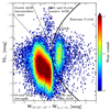 |
Fig. 14. Same as Fig. 12, but for new Galactic giant star candidates identified through their 2MASS colour and Gaia parallax with the condition Aproxy > 0.06 for the variability proxy and having MKs < −4.0 mag (see text). The star count is indicated in colour code on the right side of the figure. |
We can compare Fig. 14 with the corresponding figure obtained by Mowlavi et al. (2019) in the Magellanic Clouds (see their Figs. 4 and 7 for the LMC and SMC, respectively) and in the Milky Way from DR2 data (their Fig. 10). Our conclusions here are similar: (i) There are far fewer C-rich than O-rich stars in the Galaxy than in the Clouds. The low number of carbon stars compared to O-rich stars between the Galaxy and the Clouds agrees with the decrease in TDU efficiency with increasing metallicity, and with a higher O abundance in the envelope of Galactic AGB stars on average. On the other hand, because some of the stars located in RGB and faint AGB region in Fig. 14 might be CH and/or R-hot type stars (i.e. C-rich objects, see previous sections), we could derive a lower limit for the ratio between carbon to M (O-rich) stars. It is well known that this ratio increases with the decreasing (average) metallicity of the galaxy. The primary reason for this correlation is that less C needs to be dredged-up in a metal-poor star to enable atmospheric carbon atoms to exceed those of oxygen. We derive a ratio ∼0.05, which is very similar to the average ratio derived in the disc of M 31 (see e.g. van den Bergh 2000; Hamren et al. 2015). (ii) Moreover, the distribution of O-rich stars of the Gaia-2MASS diagram covers at any given MKs magnitude a much wider range of WRP, BP − RP − WKs, J − Ks in the Galaxy than in the Clouds. The wider distribution in both axes of the O-rich zones in Fig. 14 compared with the corresponding feature in the Clouds would result from the combined effect of O-rich AGB stars turning much later into C-rich stars in the Galaxy, and the existence of a more ample range of stellar metallicities in the Galactic sample. Moreover, Fig. 14 clearly shows the high dispersion existing in MKs for the C-rich objects at a given WRP, BP − RP − WKs, J − Ks value. Part of this dispersion in MKs is compatible with the typical range in Teff (2500−3500 K) deduced for N-type stars (Bergeat et al. 2001), and to the circumstellar extinction (which we did not consider here) preferably for the objects in the extreme C-rich region. However, the mixing of carbon stars of different populations probably also contributes significantly to this dispersion in MKs (and also in Mbol). In fact, following the method outlined in Sect. 4, we have studied the kinematics of these stars and calculated the membership probability to the halo and to the thin and thick disc of the 2659 new carbon star candidates with a Vrad measurement according to EDR3 (∼40% of the sample, i.e. 1305 objects). Figure 15 shows the corresponding Toomre diagram for these carbon stars. Of this limited sample, roughly 50% belong to the thin disc (blue circles in Fig. 15), ∼30% to the thick disc or halo (blue crosses and triangles, respectively), and the rest (∼20%) have an ambiguous membership according to our membership criteria (open blue circles). Nevertheless, we note that assuming a less strict likelihood percentage to assign membership to a population (see Sect. 4), about 25% of the stars with ambiguous membership would be thick-disc and/or halo stars. Because thick-disc and halo stars are older than thin-disc stars on average, many of these C-rich objects are very probably not intrinsic AGB carbon stars, but extrinsic C-rich giants: stars with masses lower than ∼1.5 M⊙ that have become carbon rich through the mass transfer in a binary system. An alternative to this would be the possibility that the minimum mass for the formation of an intrinsic AGB stars could be as low as 1 M⊙. Some observational evidence for this can be found in the literature (Shetye et al. 2019). This conclusion is reinforced by the scale height onto the Galactic plane that can be estimated for all the C-rich stars in Fig. 14 similarly to what was done in Sect. 2: an exponential fit gives zo ∼ 600 pc, which is much larger that the scale height derived for the intrinsic N-type AGB carbon stars that clearly belong to the thin disc (see Sect. 2).
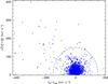 |
Fig. 15. Toomre diagram for the new candidate carbon stars. Stars are plotted according to their membership probability to belong to the thin-disc (solid blue circles), thick-disc (crosses), or halo (triangles) stellar populations. Open circles refer to stars with ambiguous membership (see text). |
Finally, Fig. 16 shows the LF derived for these new candidate carbon stars (blue histogram). We selected only objects in the C-rich region in the Gaia-2MASS diagram, that is, objects with WRP, BP − RP − WKs, J − Ks < 1.7 mag, because redder objects may be severely affected by circumstellar extinction and the BCK is rather uncertain (see Sect. 3). For these objects, we estimate an uncertainty in Mbol of ±0.30 mag because the limit adopted for the parallax error is less strict (see above). As Fig. 16 shows, the average luminosity is ⟨Mbol⟩= − 4.75 ± 0.50 mag; a fainter value than that derived for N-type stars in Sect. 3 (see Fig. 7), but still in agreement within the uncertainties. However, the reason for this lower average luminosity probably is that the selected stars have a lower metallicity on average than we studied in Sect. 3. This metallicity effect is clearly seen in the LF peak of the carbon stars in the MCs (e.g. Gullieuszik et al. 2012), which have a lower metallicity on average than the Galactic counterparts. Furthermore, this figure shows a long tail at low luminosities with Mbol values typical of RGB stars, and very bright carbon stars are also found (Mbol < −5.5 mag). These luminosity tails are populated indistinctly by stars belonging to the thin and thick discs and to halo, according to our population membership criteria. This low-luminosity tail reinforces our previous conclusion that many of the new discovered carbon stars probably have an extrinsic origin. We recall that theoretically, the minimum luminosity at which the stars become C-rich during the AGB phase is Mbol ∼ −4.0 mag (the actual value depends on the stellar metallicity; see e.g. Straniero et al. 2006), and that the low-luminosity tail in the LF of the N-type stars (see Fig. 7, top panel) can be explained with a small contribution of these stars (see also Paper I). When the LF is derived only for stars with luminosites above the RGB tip (MK ≤ −7.0 mag; see e.g. Freedman et al. 2020, the dotted line in Fig. 16), that is, stars with luminosities typical of the AGB phase, this low-luminosity tail disappears and the minimum in the LF is about Mbol ∼ −4 mag, as expected. Interesting enough, according to our kinematic study, this LF is built by stars belonging to the different stellar populations, without a significant difference among the individual LF for each stellar population. If this is confirmed by more detailed studies, the existence of intrinsic AGB carbon stars in the thick disc and halo of the Galaxy might indicate that some recent star formation episodes took place in these Galactic structures. Another possibility might be that these thick-disc and/or halo AGB carbon stars have an external origin, perhaps belonging to some of the stellar structures with peculiar kinematics recently discovered in the halo that may have been captured by our Galaxy and that very probably have had different star formation histories, such as the Gaia-Enceladus-Sausage merger, the Sequoia or Helmi streams, or the Thamnos structure (Belokurov et al. 2018; Helmi et al. 2018, 1999; Myeong et al. 2019; Koppelman et al. 2019).
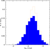 |
Fig. 16. Luminosity distribution for the new candidate carbon stars (blue) with WRP, BP − RP − WKs, J − Ks < 1.7 mag. The dotted orange line shows the luminosity function only for stars with MKs ≤ −7.0 mag, which is approximately the luminosity at the RGB tip. The bin size is 0.30 mag. |
Obviously, only a detailed and individual kinematic and spectroscopic study is able to sort and answer these questions and confirm or reject the carbon-rich nature of these candidate stars. This might be achieved with ground-based high-resolution spectra and/or space-collected Gaia/Radial Velocity Spectrometer spectra that cover the Ca II infrared triplet region at medium spectral resolution (Recio-Blanco et al., in prep.). We point out, however, that as described by Mowlavi et al. (2019)2, the carbon-rich nature of these stars might also be confirmed through the Gaia spectro-photometers, which provide low-resolution spectra that allow us to identify possible carbon molecules (C2 and CN) in their atmosphere. For these future studies, the complete list of these new carbon stars is available through the CDS database.
7. Summary
In this study we have extended the previous analysis of Abia et al. (2020, Paper I) to characterise Galactic carbon stars of different spectral types, in particular, to derive their luminosity function, location in the Galaxy, kinematics, and stellar population membership. To do this, we made use of the accurate astrometric measurements from Gaia EDR3 of the stars included in the Galactic surveys of infrared carbon stars by Chen & Yang (2012) and Chen et al. (2007), the LAMOST survey by Ji et al. (2016), and the Galactic S-type stars by Chen et al. (2019). From these surveys, we selected only stars fulfilling the criterion ϵ(ϖ)/ϖ≤0.1 having accurate infrared photometry. The final sample contains 491 carbon stars of N type, 22 of SC type, 83 of J type, 234 of R-hot type, and 276 of CH type, which represents an increase by more than a factor two in the number of objects studied with respect to Paper I. We also added 107 extrinsic and 91 intrinsic S stars from Chen et al. (2019). We derived interstellar extinctions using several Galactic models to test their impact on the derived luminosity functions. Our main results are summarised below.
(a) We find that the interstellar extinction as derived from different recent Galactic extinction models may affect the luminosity derived for individual stars, but has a negligible effect on the LF function derived for the different spectral types we studied.
(b) The average luminosity of carbon stars of N-type is ⟨Mbol⟩= − 5.04 ± 0.55 mag, which confirms our result in Paper I. However, the derived LF shows less significant tails at low and high luminosities, which partially alleviates some contradiction with theoretical predictions concerning the lower and higher mass limits for a star to become an AGB carbon star. Nevertheless, a small fraction of N-type stars show luminosities as high as Mbol ∼ −6.0 mag. Although the number of SC-type stars we analysed is still small, the LF of these stars is identical to that of N-type stars. Our kinematic study also shows that these two types of carbon stars belong to the thin-disc Galactic population.
(c) Our extended sample of J-type stars confirms that these stars are clearly less luminous than N- and SC-type stars. Their average luminosity is ⟨Mbol⟩= − 4.42 ± 0.53 mag. We find an indication of a larger scale height onto the Galactic plane for J-type stars than for N- and SC-type stars. We also confirm that the LF of R-hot stars extends over a very wide range and covers luminosities throughout the RGB (the average is ⟨Mbol⟩ = 0.05 ± 1.10 mag). This fact precludes us from assigning these types of carbon stars to a specific evolutionary stage, which favours an extrinsic origin to their carbon enhancement. The kinematic study of R-hot stars as well as their Galactic location shows features that are very similar to those of CH-type stars, which would indicate that these objects might mostly be old low-mass stars belonging to the Galactic thick disc.
(d) Intrinsic (O-rich) S stars have higher luminosities than the extrinsic ones. Their average values are ⟨Mbol⟩= − 4.42 ± 0.68 mag and ⟨Mbol⟩= − 3.52 ± 0.68 mag, respectively. In particular, the luminosities of the overwhelming majority of intrinsic S stars are higher than the predicted onset of the TDU during the AGB. For solar metallicity stars, this luminosity limit is Mbol ∼ −4.0 mag, which corresponds to stars with an initial mass above 1.3 M⊙. This result is consistent with these (Tc-rich) stars being genuine TP-AGB stars. On the other hand, both intrinsic and extrinsic S stars clearly belong to the thin-disc population.
(e) We illustrated again that the 2MASS-Gaia diagram is a powerful tool for identifying C- and O-rich AGB stars of different spectral types, according to their evolutionary stage and masses. In particular, we find that most of the carbon stars identified in the LAMOST survey are not AGB carbon stars, but probably R-hot and/or CH-type stars.
(f) We used the 2MASS-Gaia diagram to combine optical Gaia and infrared photometry to identify sub-groups of Galactic AGB stars among long-period variables, including the distinction between C-rich and O-rich stars. This study allowed us to identify 2659 stars whose C-rich nature was previously unknown.
(g) On the basis of their derived luminosities and Galactic kinematics, we argue that these new carbon stars probably constitute a mix of carbon star spectral types of intrinsic and extrinsic nature in a wide range of metallicities belonging to the thin- and thick-disc and halo populations. The full list of these new identified carbon stars is available through the CDS database for further studies to determine their actual nature and evolutionary stage. An analysis like this can be performed based on Gaia/RVS spectra, ground-based spectroscopy, and/or Gaia low-resolution spectro-photometric data.
See also, the Gaia Image of the Week: https://www.cosmos.esa.int/web/gaia/iow-20181115
Acknowledgments
This study has been partially supported by project PGC2018-095317-B-C21 financed by the MCIN/AEI FEDER “Una manera de hacer Europa”. M.R.G. and F.F. acknowledge the funding by Spanish MICIN/AEI/10.13039/501100011033 and “ERDF A way of making Europe” by the “European Union” through grant RTI2018-095076-B-C21, and the Institute of Cosmos Sciences University of Barcelona (ICCUB, Unidad de Excelencia ‘María de Maeztu’) through grant CEX2019-000918-M. This work has made use of data from the European Space Agency (ESA) mission Gaia (https://www.cosmos.esa.int/gaia), processed by the Gaia Data Processing and Analysis Consortium (DPAC, https://www.cosmos.esa.int/web/gaia/dpac/consortium). Funding for the DPAC has been provided by national institutions, in particular the institutions participating in the Gaia Multilateral Agreement. This work has been partially supported by the “Programme National de Physique Stellaire” (PNPS) of CNRS/INSU co-funded by CEA and CNES. We thank the referee Dr. N. Mowlavi for his useful comments and suggestions.
References
- Abia, C., & Wallerstein, G. 1998, MNRAS, 293, 89 [NASA ADS] [CrossRef] [Google Scholar]
- Abia, C., Domínguez, I., Gallino, R., et al. 2002, ApJ, 579, 817 [NASA ADS] [CrossRef] [Google Scholar]
- Abia, C., Domínguez, I., Gallino, R., et al. 2003, PASA, 20, 314 [CrossRef] [Google Scholar]
- Abia, C., Straniero, O., & Ventura, P. 2017, Mem. Soc. Astron. It., 88, 360 [NASA ADS] [Google Scholar]
- Abia, C., Cristallo, S., Cunha, K., de Laverny, P., & Smith, V. V. 2019, A&A, 625, A40 [CrossRef] [EDP Sciences] [Google Scholar]
- Abia, C., de Laverny, P., Cristallo, S., Kordopatis, G., & Straniero, O. 2020, A&A, 633, A135 [NASA ADS] [CrossRef] [EDP Sciences] [Google Scholar]
- Alves, D. R. 2000, ApJ, 539, 732 [NASA ADS] [CrossRef] [Google Scholar]
- Arenou, F., Grenon, M., & Gomez, A. 1992, A&A, 258, 104 [NASA ADS] [Google Scholar]
- Bailer-Jones, C. A. L., Rybizki, J., Fouesneau, M., Demleitner, M., & Andrae, R. 2021, VizieR Online Data Catalog: I/352 [Google Scholar]
- Belokurov, V., Erkal, D., Evans, N. W., Koposov, S. E., & Deason, A. J. 2018, MNRAS, 478, 611 [Google Scholar]
- Bergeat, J., Knapik, A., & Rutily, B. 2001, A&A, 369, 178 [NASA ADS] [CrossRef] [EDP Sciences] [Google Scholar]
- Bergeat, J., Knapik, A., & Rutily, B. 2002, A&A, 390, 967 [NASA ADS] [CrossRef] [EDP Sciences] [Google Scholar]
- Castellani, V., Degl’Innocenti, S., Girardi, L., et al. 2000, A&A, 354, 150 [NASA ADS] [Google Scholar]
- Chan, S. J., & Kwok, S. 1990, A&A, 237, 354 [NASA ADS] [Google Scholar]
- Chen, P. S., & Chen, W. P. 2003, AJ, 125, 2215 [NASA ADS] [CrossRef] [Google Scholar]
- Chen, P. S., & Yang, X. H. 2012, AJ, 143, 36 [NASA ADS] [CrossRef] [Google Scholar]
- Chen, P.-S., Yang, X.-H., & Zhang, P. 2007, AJ, 134, 214 [NASA ADS] [CrossRef] [Google Scholar]
- Chen, P. S., Liu, J. Y., & Shan, H. G. 2019, AJ, 158, 22 [NASA ADS] [CrossRef] [Google Scholar]
- Claussen, M. J., Kleinmann, S. G., Joyce, R. R., & Jura, M. 1987, ApJS, 65, 385 [NASA ADS] [CrossRef] [Google Scholar]
- Clayton, G. C. 2012, J. Am. Assoc. Var. Star Obs., 40, 539 [NASA ADS] [Google Scholar]
- Cristallo, S., Piersanti, L., Straniero, O., et al. 2011, ApJS, 197, 17 [NASA ADS] [CrossRef] [Google Scholar]
- Cristallo, S., Straniero, O., Piersanti, L., & Gobrecht, D. 2015, ApJS, 219, 40 [Google Scholar]
- Cutri, R. M., Skrutskie, M. F., van Dyk, S., et al. 2003, VizieR Online Data Catalog: II/246 [Google Scholar]
- Dove, J. B., & Thronson, H. A., Jr. 1993, ApJ, 411, 632 [NASA ADS] [CrossRef] [Google Scholar]
- Drimmel, R., Cabrera-Lavers, A., & López-Corredoira, M. 2003, A&A, 409, 205 [NASA ADS] [CrossRef] [EDP Sciences] [Google Scholar]
- Escorza, A., Boffin, H. M. J., Jorissen, A., et al. 2017, A&A, 608, A100 [NASA ADS] [CrossRef] [EDP Sciences] [Google Scholar]
- Freedman, W. L., Madore, B. F., Hoyt, T., et al. 2020, ApJ, 891, 57 [Google Scholar]
- Frogel, J. A., Persson, S. E., & Cohen, J. G. 1980, ApJ, 239, 495 [NASA ADS] [CrossRef] [Google Scholar]
- Gaia Collaboration (Helmi, A., et al.) 2018, VizieR Online Data Catalog: J/A+A/616/A12 [Google Scholar]
- Gaia Collaboration (Antoja, T., et al.) 2021, A&A, 649, A8 [EDP Sciences] [Google Scholar]
- Girardi, L., Groenewegen, M. A. T., Hatziminaoglou, E., & da Costa, L. 2005, A&A, 436, 895 [NASA ADS] [CrossRef] [EDP Sciences] [Google Scholar]
- Green, G. M., Schlafly, E., Zucker, C., Speagle, J. S., & Finkbeiner, D. 2019, ApJ, 887, 93 [NASA ADS] [CrossRef] [Google Scholar]
- Groenewegen, M. A. T., Sevenster, M., Spoon, H. W. W., & Pérez, I. 2002, A&A, 390, 511 [NASA ADS] [CrossRef] [EDP Sciences] [Google Scholar]
- Guandalini, R., Busso, M., Ciprini, S., Silvestro, G., & Persi, P. 2006, A&A, 445, 1069 [NASA ADS] [CrossRef] [EDP Sciences] [Google Scholar]
- Gullieuszik, M., Groenewegen, M. A. T., Cioni, M.-R. L., et al. 2012, A&A, 537, A105 [NASA ADS] [CrossRef] [EDP Sciences] [Google Scholar]
- Gupta, R., Singh, H. P., Volk, K., & Kwok, S. 2004, ApJS, 152, 201 [NASA ADS] [CrossRef] [Google Scholar]
- Habing, H. J., & Olofsson, H. 2004, Asymptotic Giant Branch Stars (New York: Springer) [CrossRef] [Google Scholar]
- Hamren, K. M., Rockosi, C. M., Guhathakurta, P., et al. 2015, ApJ, 810, 60 [NASA ADS] [CrossRef] [Google Scholar]
- Helmi, A., White, S. D. M., de Zeeuw, P. T., & Zhao, H. 1999, Nature, 402, 53 [Google Scholar]
- Helmi, A., Babusiaux, C., Koppelman, H. H., et al. 2018, Nature, 563, 85 [Google Scholar]
- Izzard, R. G., & Tout, C. A. 2004, MNRAS, 350, L1 [Google Scholar]
- Izzard, R. G., Jeffery, C. S., & Lattanzio, J. 2007, A&A, 470, 661 [NASA ADS] [CrossRef] [EDP Sciences] [Google Scholar]
- Izzard, R. G., Jeffery, C. S., & Lattanzio, J. 2008, in Evolution and Nucleosynthesis in AGB Stars, eds. R. Guandalini, S. Palmerini, & M. Busso, AIP Conf. Ser., 1001, 33 [NASA ADS] [Google Scholar]
- Ji, W., Cui, W., Liu, C., et al. 2016, ApJS, 226, 1 [NASA ADS] [CrossRef] [Google Scholar]
- Karakas, A. I., & Lattanzio, J. C. 2014, PASA, 31, e030 [NASA ADS] [CrossRef] [Google Scholar]
- Katz, D., Sartoretti, P., Cropper, M., et al. 2019, A&A, 622, A205 [NASA ADS] [CrossRef] [EDP Sciences] [Google Scholar]
- Kerschbaum, F., Lebzelter, T., & Mekul, L. 2010, A&A, 524, A87 [NASA ADS] [CrossRef] [EDP Sciences] [Google Scholar]
- Knapp, G., Pourbaix, D., & Jorissen, A. 2001, A&A, 371, 222 [NASA ADS] [CrossRef] [EDP Sciences] [Google Scholar]
- Koppelman, H. H., Helmi, A., Massari, D., Price-Whelan, A. M., & Starkenburg, T. K. 2019, A&A, 631, L9 [NASA ADS] [CrossRef] [EDP Sciences] [Google Scholar]
- Lallement, R., Babusiaux, C., Vergely, J. L., et al. 2019, A&A, 625, A135 [NASA ADS] [CrossRef] [EDP Sciences] [Google Scholar]
- Le Bertre, T., Tanaka, M., Yamamura, I., Murakami, H., & MacConnell, D. J. 2005, PASP, 117, 199 [NASA ADS] [CrossRef] [Google Scholar]
- Lebzelter, T., Mowlavi, N., Marigo, P., et al. 2018, A&A, 616, L13 [NASA ADS] [CrossRef] [EDP Sciences] [Google Scholar]
- Lindegren, L., Klioner, S. A., Hernández, J., et al. 2021, A&A, 649, A2 [EDP Sciences] [Google Scholar]
- Luri, X., Palmer, M., Arenou, F., et al. 2014, A&A, 566, A119 [NASA ADS] [CrossRef] [EDP Sciences] [Google Scholar]
- Marigo, P., Girardi, L., Bressan, A., et al. 2017, ApJ, 835, 77 [Google Scholar]
- Marigo, P., Bossini, D., Trabucchi, M., et al. 2022, ApJS, 258, 43 [NASA ADS] [Google Scholar]
- Marshall, D. J., Robin, A. C., Reylé, C., Schultheis, M., & Picaud, S. 2006, A&A, 453, 635 [NASA ADS] [CrossRef] [EDP Sciences] [Google Scholar]
- McClure, R. D. 1984, in Observational Tests of the Stellar Evolution Theory, eds. A. Maeder, & A. Renzini, IAU Symp., 105, 187 [NASA ADS] [CrossRef] [Google Scholar]
- Messineo, M., & Brown, A. G. A. 2019, AJ, 158, 20 [NASA ADS] [CrossRef] [Google Scholar]
- Miller, G. E., & Scalo, J. M. 1979, ApJS, 41, 513 [Google Scholar]
- Mowlavi, N., Lecoeur-Taïbi, I., Lebzelter, T., et al. 2018, A&A, 618, A58 [NASA ADS] [CrossRef] [EDP Sciences] [Google Scholar]
- Mowlavi, N., Trabucchi, M., & Lebzelter, T. 2019, https://doi.org/10.5281/zenodo.3243501 [Google Scholar]
- Myeong, G. C., Vasiliev, E., Iorio, G., Evans, N. W., & Belokurov, V. 2019, MNRAS, 488, 1235 [Google Scholar]
- Neugebauer, G., Habing, H. J., van Duinen, R., et al. 1984, ApJ, 278, L1 [NASA ADS] [CrossRef] [Google Scholar]
- Nordström, B., Mayor, M., Andersen, J., et al. 2004, A&A, 418, 989 [Google Scholar]
- Reid, M. J., & Honma, M. 2014, ARA&A, 52, 339 [NASA ADS] [CrossRef] [Google Scholar]
- Rybizki, J., Green, G. M., Rix, H.-W., et al. 2022, MNRAS, 510, 2597 [NASA ADS] [CrossRef] [Google Scholar]
- Salaris, M., & Girardi, L. 2002, MNRAS, 337, 332 [NASA ADS] [CrossRef] [Google Scholar]
- Samus, N. N., & Durlevich, O. V. 2004, VizieR Online Data Catalog: II/250 [Google Scholar]
- Schechter, P. L., Cook, K. H., Aaronson, M., & Blanco, V. M. 1987, BAAS, 19, 1069 [NASA ADS] [Google Scholar]
- Schönrich, R. 2012, MNRAS, 427, 274 [Google Scholar]
- Shetye, S., Van Eck, S., Jorissen, A., et al. 2018, A&A, 620, A148 [NASA ADS] [CrossRef] [EDP Sciences] [Google Scholar]
- Shetye, S., Goriely, S., Siess, L., et al. 2019, A&A, 625, L1 [NASA ADS] [CrossRef] [EDP Sciences] [Google Scholar]
- Shetye, S., Van Eck, S., Jorissen, A., et al. 2021, A&A, 650, A118 [NASA ADS] [CrossRef] [EDP Sciences] [Google Scholar]
- Siess, L., Dufour, E., & Forestini, M. 2000, A&A, 358, 593 [Google Scholar]
- Skrutskie, M. F., Cutri, R. M., Stiening, R., et al. 2006, AJ, 131, 1163 [NASA ADS] [CrossRef] [Google Scholar]
- Soszyński, I., Gieren, W., & Pietrzyński, G. 2005, PASP, 117, 823 [Google Scholar]
- Stancliffe, R. J., Izzard, R. G., & Tout, C. A. 2005, MNRAS, 356, L1 [Google Scholar]
- Straniero, O., Domínguez, I., Cristallo, S., & Gallino, R. 2003, PASA, 20, 389 [Google Scholar]
- Straniero, O., Gallino, R., & Cristallo, S. 2006, Nucl. Phys. A, 777, 311 [NASA ADS] [CrossRef] [Google Scholar]
- Trams, N. R., van Loon, J. T., Zijlstra, A. A., et al. 1999, A&A, 344, L17 [NASA ADS] [Google Scholar]
- Uttenthaler, S. 2013, A&A, 556, A38 [NASA ADS] [CrossRef] [EDP Sciences] [Google Scholar]
- Uttenthaler, S., & Lebzelter, T. 2010, A&A, 510, A62 [NASA ADS] [CrossRef] [EDP Sciences] [Google Scholar]
- van den Bergh, S. 2000, The Galaxies of the Local Group (Cambridge: Cambridge University Press) [Google Scholar]
- Van Eck, S., & Jorissen, A. 1999, A&A, 345, 127 [NASA ADS] [Google Scholar]
- Van Eck, S., Jorissen, A., Udry, S., Mayor, M., & Pernier, B. 1998, A&A, 329, 971 [NASA ADS] [Google Scholar]
- van Loon, J. T., Zijlstra, A. A., & Groenewegen, M. A. T. 1999, A&A, 346, 805 [NASA ADS] [Google Scholar]
- Vanture, A. D., Smith, V. V., Lutz, J., et al. 2007, PASP, 119, 147 [NASA ADS] [CrossRef] [Google Scholar]
- Wallerstein, G., & Knapp, G. R. 1998, ARA&A, 36, 369 [NASA ADS] [CrossRef] [Google Scholar]
- Wood, P. R. 2000, PASA, 17, 18 [Google Scholar]
- Zamora, O., Abia, C., Plez, B., Domínguez, I., & Cristallo, S. 2009, A&A, 508, 909 [NASA ADS] [CrossRef] [EDP Sciences] [Google Scholar]
- Zhao, G., Zhao, Y., Chu, Y., Jing, Y., & Deng, L. 2012, ArXiv e-prints [arXiv:1206.3569] [Google Scholar]
All Tables
All Figures
|
Fig. 1. Comparison of the histogram of the Gaia DR3 parallaxes in the initial sample of stars (dashed line) with the parallaxes deduced from the Bailer-Jones et al. (2021) distances adopted after filtering the sample according to our quality parallax criteria (continuous line). The bin size is 0.1 mas (see text). |
| In the text | |
|
Fig. 2. Top: location of the stellar sample of carbon stars around the Sun. The Sun is placed at (X, Y) = (0, 0). Stars are taken from the surveys by Chen et al. (2007) and Chen & Yang (2012). Blue dots show normal N-type carbon stars; red dots represent J-type stars, and cyan dots show stars of unknown type according to Chen & Yang (2012) that are labelled possible carbon stars in SIMBAD. Bottom: distribution above or below the Galactic plane vs. galactocentric distance. The Sun is at R = 8.34 kpc. The typical uncertainty in the (X, Y, Z) coordinates is ±20 pc, and it is ±50 pc for the galactocentric distance (see text). |
| In the text | |
|
Fig. 3. Same as Fig. 2 for the carbon stars in the LAMOST survey (Ji et al. 2016). Solid blue dots show N-type carbon stars, grey dots represent CH-type stars, and brown dots show R-hot stars. The limits of the X- and Y-axes and R coordinates are different from Fig. 2. |
| In the text | |
|
Fig. 4. Same as Fig. 2 for the S stars in Chen et al. (2019). Solid black circles show extrinsic stars, and purple circles show intrinsic stars. The limits of the X- and Y-axes and R coordinates are different from Fig. 2. |
| In the text | |
|
Fig. 5. Histograms showing the distribution (normalised to the maximum number of stars) of the |Z|-coordinate for the different spectral types. From top to bottom: normal N-type carbon stars (blue), extrinsic (black) and intrinsic (purple) S stars, J-type stars (red), and R-type stars (brown). The X-axis for the R-type stars is different. For N-type normal carbon stars, orange lines show exponential fits to the distribution with scale heights zo = 260, 220, and 180 pc from top to bottom. Similar fits give an estimate of the scale-height for the other spectral types (see text). The bin size is 20 pc. |
| In the text | |
|
Fig. 6. Comparison of the interstellar extinction AV derived from the different Galactic extinction models used in this study. The dashed orange line shows the 1:1 relation. |
| In the text | |
|
Fig. 7. Luminosity distributions (coloured histograms) derived in this study for the different spectral types of Galactic carbon stars (CH-type stars are not shown). The bin size is 0.25 mag. The range in luminosity is different for the R-hot stars that are fainter. For comparison, the corresponding histogram obtained in Paper I for each spectral type is shown in each panel (dotted histograms). |
| In the text | |
|
Fig. 8. Luminosity distributions derived for the S stars of this study. Purple shows intrinsic S stars, and black shows extrinsic S stars. The bin at Mbol ∼ −2.0 mag. corresponds to the star Hen 4−16 alone, which is quoted in SIMBAD as a possible S star. The bin size is 0.25 mag. |
| In the text | |
|
Fig. 9. Toomre diagram for the selected carbon stars of this study. The colour symbols are the same as in Fig. 1. Stars are plotted according to their membership probability (> 80%) to belong to the thin disc (solid circles), thick disc (crosses), or halo (triangles) stellar population. Open circles show stars with ambiguous membership (see text). Dashed lines indicate |
| In the text | |
|
Fig. 10. Same as Fig. 9 for extrinsic (black) and intrinsic (purple) S stars. The star HD 160379 (open circle) has an ambiguous Galactic membership population between thick disc and halo according to our criteria (see text). |
| In the text | |
|
Fig. 11. Same as Fig. 9 for the CH-type stars in the LAMOST sample (Ji et al. 2016) together with the R-hot stars also in LAMOST and those included in Paper I (grey and brown symbols, respectively). A significant number of stars classified in LAMOST as R-hot type have ambiguous Galactic population membership (open brown circles), mainly between the thin and thick disc (see text). |
| In the text | |
|
Fig. 12. Gaia-2MASS diagram for our main star sample. The curved line delineates the theoretical limit between O-rich (left of the line) and C-rich AGB stars (right of the line). Dashed lines separate sub-groups of stars as indicated in the figure. The colour code for the different AGB types is shown in the bottom right corner. Open blue circles show N-type stars for clarity. Several SC-type stars (green circles) and J-type stars (red circles) are placed in the C-rich zone, but cannot be distinguished in the figure because of crowding. The uncertainty in MKs typically is ±0.23 mag. |
| In the text | |
|
Fig. 13. Same as Fig. 12 for the carbon stars in the LAMOST sample by Ji et al. (2016). Grey circles show CH-type stars, brown circles show R-hot stars, blue circles show normal N-type stars, open blue circles show possible N-type stars, and open orange circles show carbon stars of unknown type. For completeness, we show (cyan circles) the carbon stars in Chen & Yang (2012) with (J − Ks) > 2.5 mag. The inset shows a zoom of a small area in the location of the R-hot and CH-type stars (see text). |
| In the text | |
|
Fig. 14. Same as Fig. 12, but for new Galactic giant star candidates identified through their 2MASS colour and Gaia parallax with the condition Aproxy > 0.06 for the variability proxy and having MKs < −4.0 mag (see text). The star count is indicated in colour code on the right side of the figure. |
| In the text | |
|
Fig. 15. Toomre diagram for the new candidate carbon stars. Stars are plotted according to their membership probability to belong to the thin-disc (solid blue circles), thick-disc (crosses), or halo (triangles) stellar populations. Open circles refer to stars with ambiguous membership (see text). |
| In the text | |
|
Fig. 16. Luminosity distribution for the new candidate carbon stars (blue) with WRP, BP − RP − WKs, J − Ks < 1.7 mag. The dotted orange line shows the luminosity function only for stars with MKs ≤ −7.0 mag, which is approximately the luminosity at the RGB tip. The bin size is 0.30 mag. |
| In the text | |
Current usage metrics show cumulative count of Article Views (full-text article views including HTML views, PDF and ePub downloads, according to the available data) and Abstracts Views on Vision4Press platform.
Data correspond to usage on the plateform after 2015. The current usage metrics is available 48-96 hours after online publication and is updated daily on week days.
Initial download of the metrics may take a while.