| Issue |
A&A
Volume 664, August 2022
|
|
|---|---|---|
| Article Number | A99 | |
| Number of page(s) | 26 | |
| Section | Stellar structure and evolution | |
| DOI | https://doi.org/10.1051/0004-6361/202243294 | |
| Published online | 10 August 2022 | |
XMM-Newton and Swift observations of supergiant high mass X-ray binaries
1
Department of astronomy, University of Geneva, chemin d’Écogia, 16, 1290 Versoix, Switzerland
e-mail: This email address is being protected from spambots. You need JavaScript enabled to view it.
2
INAF-OAR, Via Frascati, 33, 00078 Monte Porzio Catone RM, Italy
3
INAF, Osservatorio Astronomico di Brera, Via E. Bianchi 46, 23807 Merate, Italy
Received:
9
February
2022
Accepted:
29
April
2022
Abstract
Wind-fed supergiant X-ray binaries are precious laboratories not only to study accretion under extreme gravity and magnetic field conditions, but also to probe the still highly debated properties of massive star winds. These include clumps, originating from the inherent instability of line driven winds, and larger structures. In this paper we report on the results of the last (and not yet published) monitoring campaigns that our group has been carrying out since 2007 with both XMM-Newton and the Swift Neil Gehrels observatory. Data collected with the EPIC cameras on board XMM-Newton allow us to carry out a detailed hardness-ratio-resolved spectral analysis that can be used as an efficient way to detect spectral variations associated with the presence of clumps. Long-term observations with the XRT on board Swift, evenly sampling the X-ray emission of supergiant X-ray binaries over many different orbital cycles, are exploited to look for the presence of large-scale structures in the medium surrounding the compact objects. These can be associated either with corotating interaction regions or with accretion and/or photoionization wakes, and with tidal streams. The results reported in this paper represent the outcomes of the concluded observational campaigns we carried out on the supergiant X-ray binaries 4U 1907+09, IGR J16393−4643, IGR J19140+0951, and XTE J1855−026, and on the supergiant fast X-ray transients IGR J17503−2636, IGR J18410−0535, and IGR J11215−5952. All results are discussed in the context of wind-fed supergiant X-ray binaries and ideally serve to optimally shape the next observational campaigns aimed at sources in the same classes. We show in one of the Appendices that IGR J17315−3221, preliminarily classified in the literature as a possible supergiant X-ray binary discovered by INTEGRAL, is the product of a data analysis artifact and should thus be disregarded for future studies.
Key words: X-rays: binaries / stars: neutron / X-rays: individuals: 4U 1907+097 / X-rays: individuals: IGR J19140+0951 / X-rays: individuals: IGR J17503−2636 / X-rays: individuals: IGR J17315+3221
© C. Ferrigno et al. 2022
 Open Access article, published by EDP Sciences, under the terms of the Creative Commons Attribution License (https://creativecommons.org/licenses/by/4.0), which permits unrestricted use, distribution, and reproduction in any medium, provided the original work is properly cited.
This article is published in open access under the Subscribe-to-Open model. This email address is being protected from spambots. You need JavaScript enabled to view it. to support open access publication.
1. Introduction
Supergiant X-ray binaries (SgXBs) are a subclass of high mass X-ray binaries (HMXBs) most commonly hosting a neutron star (NS) accreting from the wind of an OB supergiant. For the bulk of known system in this class, the compact object accretes from the material that the massive companion loses through a fast and dense wind. The interest in SgXBs has been revived in recent years due to the recognition that they are key laboratories to investigate properties of the still highly debated massive star winds using the NS as a probe, especially in the domain of macro-clumping and large-scale structures (see, e.g., Martínez-Núñez et al. 2017; Bozzo et al. 2016, and discussions therein).
In the framework of this renewed interest, our group has started a number of monitoring programs of several SgXBs with both XMM-Newton and Swift to look for spectral variability in the X-ray emission of these sources that could be ascribed to the presence of massive structures in the stellar winds approaching the compact object and causing episodes of enhanced X-ray emission and/or obscuration of the high energy source (clumps or even larger structures; see, e.g., Puls et al. 2008, and later in this section). Our monitoring program covers both sources within the subclass of the classical SgXBs, showing a moderate X-ray variability, up to a factor of ∼103 between quiescent and more active periods, and the supergiant fast X-ray transients (SFXTs), showing a much more pronounced X-ray variability up to a factor of 106 between quiescence and the brightest outbursts (see, e.g., Walter et al. 2015; Romano et al. 2015, and references therein).
As discussed by Bozzo et al. (2017a), hunting for spectral variations during SgXBs flares and outbursts to study the smaller stellar wind clumps requires sufficiently long and uninterrupted observations of these sources with X-ray instruments endowed with a large effective area in the soft X-ray domain (∼3 keV). This is so because the time intervals for the spectral extraction have a typical duration of a few hundred to thousands of seconds, and enough X-ray counts need to be collected to perform meaningful spectral fits and to disentangle both continuum and absorption column density variations. These integration times are set by the usual duration of flares and outbursts, which is limited to a few hours at the most, and the need for as many probed time intervals as possible along the event rise and decay to study the dynamics of the accretion process (see, e.g., Bozzo et al. 2011, 2013a). To date, the EPIC cameras on board XMM-Newton (Jansen et al. 2001) have proven to be the most effective instruments to pursue this goal (Bozzo et al. 2017a). The techniques we deployed to look for the spectral variability in the XMM-Newton data of classical SgXBs and SFXTs comprise an adaptively rebinned hardness ratio (HR) of the source-energy-resolved light curves and a Bayesian block automatized selection of the time intervals corresponding to the most significant changes in the HR for the spectral extraction. These techniques are exhaustively described in a number of our previous papers, where we also illustrate the results obtained from several classical SgXBs and SFXTs (see, e.g., Bozzo et al. 2010, 2011, 2013a, 2015, 2017a; Ferrigno et al. 2020, and references therein). The HR-resolved spectral analysis that we have carried out so far reveals that during sufficiently bright flares and outbursts from the SgXBs we recorded an increase in the absorption column density preceding the brightening event and a decrease in the absorption close to the peak of the event. In several cases we also observed a new increase in the absorption column density toward the end of the flare–outburst, as well as a change in the centroid energy of the iron line feature that is produced due to the fluorescence of the accretion X-rays onto the surrounding stellar wind material. In a few observations, episodes of enhanced absorption of the X-rays from the NS have been observed for as long as a few hundred seconds, also without being in coincidence with either a flare or an outburst. The physical picture that emerged from these results is that accretion in all analyzed SgXBs is compatible with it occurring from a clumpy wind, where dense structures approach the compact object before being accreted and cause the local absorption column density to rise before the flare–outburst. The decrease in the absorption column density toward the peak of the event is ascribed to the photoionization effect of the enhanced X-rays onto the clump material, while the recombination following the beginning of the X-ray flux decay after the peak of the flare–outburst can explain the subsequent re-increase in the local absorption column density back to pre-rebrightening values. This scenario is more quantitatively confirmed for those cases where also a change in the centroid energy of the iron line is measured as this provides a clearer identification of the ionization status of the stellar wind around the compact object (see, e.g., Bozzo et al. 2011, and references therein). Those episodes in which only a transient absorption of X-rays is visible without being associated with a rebrightening event are commonly ascribed to clumps passing in front of the compact object along the line of sight of the observer without intercepting its orbit and being (at least) partly accreted.
The results obtained from several observations of classical SgXBs and SFXTs suggest that the features measured through the HR-resolved spectral analysis are quite similar for both classes of objects. Although clumps are thus a key ingredient for the accretion in both subclasses of sources, it seems necessary to assume that additional mechanisms are at work in SFXTs to explain their much more prominent X-ray variability. So far, the considered mechanisms include gatings due to the NS rotation and magnetic field (Bozzo et al. 2008, 2017b) and the onset of a long-standing settling accretion regime (Shakura et al. 2012).
It should be mentioned that a number of flares, especially from the SFXTs, did not show evidence of substantial absorption column density enhancements (see, e.g., Bozzo et al. 2015). These events have been interpreted as being triggered by the above “additional mechanisms” without the (significant) intervention of clumps or as being observed through a direction such that our line of sight did not pass through (or intercept) the clump. To date, the geometrical shape of the clumps and other relevant parameters (e.g., spatial extents in general, masses, and densities) are poorly constrained, and thus geometrical effects have to be folded in the study of the accretion process as additional uncertainties.
In addition to clumps, other massive structures are known to populate the accretion environments of NSs in SgXBs and can thus contribute to enhancing the X-ray variability of these systems. Among such structures there are the corotating interaction regions (CIRs), which are extended structures originating from the surface of the supergiant star and extending up to several stellar radii. The CIRs are characterized by mild overdensity ratios compared to the rest of the stellar wind, and since they do not perfectly co-rotate with the supergiant star the interception of the NS with one of these structures could result in periodic enhancements of the X-ray luminosity and absorption column density at specific orbital phases (thus also giving rise to super-orbital modulations; see Bozzo et al. 2016, and references therein).
Similar enhancements at fixed orbital phases can also be produced by the presence of accretion and photoionization wakes and by tidal streams. Accretion wakes are dense structures partly surrounding the compact object and produced by the focusing of the stellar wind medium by the NS gravitational influence, while photoionization wakes are regions where the overdensity (compared to the surrounding accretion medium) is due to the X-ray photoionization of the stellar wind and its partial stagnation. Finally, tidal streams are possible only in those systems where the supergiant companion nearly fills its Roche lobe (see, e.g., Manousakis & Walter 2011; Grinberg et al. 2017; Kretschmar et al. 2019, and references therein).
The study of orbital-phase-dependent structures requires long-term observations covering as many orbital periods as possible. The reason is that the eventual spectral variability recorded from the data on a single specific orbital phase is likely to be dominated by the effect of short-term variations in the accretion environment associated with clumps (thousands of seconds to hours). Averaging data at the same orbital phase but collected over many different orbits ensures that the short-term variability of the clumps is “washed away” and spectral changes can be most likely ascribed to the presence of large-scale stable structures. For these reasons, relatively short snapshots with the narrow-field instrument X-ray Telescope (XRT, Burrows et al. 2005) on board the Neil Gehrels Swift Observatory (Swift, Gehrels et al. 2004) carried out over several months (considering that the typical orbital period of a SgXB is a few dozen days at most) provide us the most effective strategy to collect the required data for the analysis of large-scale wind structures in classical SgXBs and SFXTs.
In this paper we report on several XMM-Newton observations of classical SgXBs and SFXTs that were either not published or not yet analyzed with our techniques (see above) to reveal spectral variations that can be associated with the presence of clumps. These results complement those reported previously in our papers on this topic. Furthermore, we report for the first time on the analysis of monitoring observational campaigns performed with Swift/XRT on several classical SgXBs in order to investigate possible spectral variability as a function of orbital phase. Although some of these data were already reported elsewhere, we systematically apply a technique that can most effectively be used to reveal the presence of large-scale structures around the compact objects in these systems. We discuss our results in the framework of wind accretion in neutron star SgXBs.
The sources investigated in this paper are listed in Table 1. We note that only in the case of 4U 1907+09 are both kinds of observations available to study the short- and long-term spectral variability associated with clumps and large-scale wind structures. In all other cases, either focused XMM-Newton observations or longer-term Swift/XRT data have been collected. For XTE J1855−026, XRT data have been exploited to search for the short-term spectral variability associated with clumps because the observations were performed during a few rare bright outbursts of the source. In the case of IGR J17503−2636, the data from the XRT observational campaign could not be folded on the source orbital period as it is still unknown.
Properties of the sources studied in this paper.
In Sect. 2 we describe the general analysis methods for Swift and XMM-Newton. In Sect. 3 we briefly describe each source in our sample with an overview of the data sets available for each of them; we give details of the specific analysis methods and the results we obtained; and present our discussion. In Sect. 4 we draw the conclusions of our work.
2. General data analysis methods
2.1. Swift
All Swift data were uniformly processed and analyzed using the standard software (FTOOLS1 v6.29b), calibration (CALDB2 20210915), and methods. The Swift/XRT data were processed and filtered with the task XRTPIPELINE (v0.13.6).
For all sources with available XRT data, we first extracted the average spectrum in each XRT observation to measure the 0.3–10 keV flux. Then we computed, for each observation, the HR value using the source count rate in the 0.3–4 keV and 4–10 keV energy bands. If an orbital period was available (4U 1907+09, IGR J16393−4643, IGR J19140+0951), we calculated the orbital phase corresponding to each XRT observation and chose eight phase bins that would yield a comparable number of source counts (4U 1907+09: ∼2700 counts; IGR J16393−4643: ∼1300 counts; IGR J19140+0951: ∼900 counts). Using the above energy bands, we calculated the hardness ratio for each phase bin and plotted the hardness ratio as a function of the orbital phase.
We note that the XRT observations are generally composed of up to three snapshots with typical exposures of 300–1000 s. Therefore, none of the XRT observations is suitable to look for the known pulsations of some of the target sources (see Sect. 3); however, computing the HR in each of them rather than in the single snapshots ensures that the effect of the pulse period energy dependence on the HR is averaged out. This is further strengthened by the fact that several different observations are averaged together in order to compute the HR in the defined orbital phase bins.
In order to comprehensively investigate possible spectral variability in different orbital phase bins, as suggested by the HR variations, we extracted different source spectra for each of these bins, grouped them so as to have at least one count per bin, and fit them by using a simple absorbed power-law model in XSPEC version 12.12.0. For the absorption column density, we adopted the TBABS component with wilm abundances (Wilms et al. 2000) and vern cross sections (Verner et al. 1996).
2.2. XMM-Newton
All XMM-Newton observation data files (ODFs) were processed by using the XMM-Newton Science Analysis System (SAS 20.0.0), following standard procedures3. We filtered out background flaring time intervals due to cosmic protons with the follwing method. We extract the 10–12 keV EPIC-pn light curve binned at 100 s, then we select the count rate values belonging to the first 70% percentile, we fit a Gaussian distribution to them, and we exclude the count-rate values with less than 0.1% probability of belonging to such distribution. We retained, however, any time interval with a count rate below 0.6 counts per second.
The regions adopted for the extraction of all source and background scientific products (light curves and spectra) were chosen by checking where the instrument point spread function includes an optimal fraction of the photons specific to each source, or by picking the maximum allowed radius when the observation was carried out in small-window mode (see below for details for each source). We extracted the spectra and light curves of the three EPIC cameras together with the associated ancillary and response matrices, using standard procedures.
We grouped all EPIC spectra using the algorithms described in Kaastra & Bleeker (2016) and adopted as baseline model a power law affected at the lower energies by photoelectric absorption. In addition to that used for Swift/XRT data, we generally add an absorber partly covering the source (pcfabs in XSPEC). To find the best-fit parameters, we minimized the Cash statistics with background correction (Cstat in XSPEC), using a standard Levenberg–Marquardt algorithm based on the CURFIT routine from Bevington and then computed uncertainties using a Markov chain Monte Carlo procedure exploiting the Goodman–Weare algorithm. We used 60 walkers, a burning phase of 6000, and a chain length of 36 000. Uncertainties were found by computing the appropriate percentiles in the posterior distributions. As customary, we used a logarithmic prior for normalization and column density, and a linear prior for the slope and covering fraction.
For each source observed by XMM-Newton, we extracted the EPIC-pn, MOS1, and MOS2 light curves in two energy bands by computing the band limits as the median photon energy in the EPIC-pn camera to optimize the computation of the hardness ratio (HR). We summed together all the EPIC light curves of each source to improve the statistical uncertainties and to compute the adaptively rebinned hardness ratio (HR; see Bozzo et al. 2013b, for a description of the adaptive rebinning method). A typical minimum signal-to-noise ratio (S/N) of 25 was achieved for the different sources in each of the time bins of the summed light curves. We determined periods in which the HR changes significantly by a Bayesian block analysis optimized to identify the most relevant HR variations with a negligible number of false positives (we used the fitness for point measurements and ncp_prior = 3.98, see Scargle et al. 2013, Sect 3.3). In each of the identified intervals, we extracted the corresponding spectra using appropriate extraction regions as for the averaged spectra and constructed the corresponding ancillary and response matrices.
All uncertainties in the measured parameters from each source in the following subsections are indicated at a 68% confidence level, unless stated otherwise.
3. Description of targets, analysis results, and discussion
3.1. 4U 1907+09
4U 1907+09 is a classical supergiant X-ray binary discovered in the 1970s by the Uhuru satellite (Forman et al. 1978; Giacconi et al. 1972) and hosting a slowly rotating NS (the spin period is ∼437 s; Makishima et al. 1984) orbiting a O8/O9 Ia supergiant (van Kerkwijk et al. 1989; Cox et al. 2005). The system orbital period is measured at ∼8.38 d (Marshall & Ricketts 1980; in ’t Zand et al. 1998). The NS in this system is known to undergo episodes of spin torque reversal (Fritz et al. 2006; Inam et al. 2009), to display occasional quasi-periodic oscillations at a frequency of about 65 mHz (in ’t Zand et al. 1998; Mukerjee et al. 2001), and to be endowed with a magnetic field strength of ∼2 × 10¹² G (the estimate is provided by the presence of a cyclotron scattering feature in the source X-ray spectrum with a centroid energy of ∼19 keV; see, e.g., Hemphill et al. 2013; Varun et al. 2019, and references therein). As most highly magnetized NSs in HMXBs, the compact object in 4U 1907+09 features a complex pulse profile, which is both energy and luminosity dependent. This has been the central subject of several literature works on the source (see, e.g., Mukerjee et al. 2001; Rivers et al. 2010; Şahiner et al. 2012; Fürst et al. 2012). In the X-ray band this source displays a dipping behavior which has been known for decades, but is yet not clearly understood (in ’t Zand et al. 1997; Doroshenko et al. 2012).
3.1.1. Data analysis and results
Our as-yet-unpublished monitoring campaign on 4U 1907+09 with Swift/XRT was performed at a pace of two observations per week, each 1 ks long, spanning from February to September 2015 with OBServation IDentifier (OBSID) 33483. The full log of the XRT observations is provided in Table C.1. The 0.3–10 keV flux obtained by fitting the average spectrum of the source in each XRT observation with an absorbed power law are reported in Table C.1. We calculated the orbital phase corresponding to each XRT observation by using the source ephemerides published by in ’t Zand et al. (1998; see Table 1) and grouped these observations in eight phase bins yielding a comparable number of source counts in each bin (∼2700 counts). Figure 1a shows the hardness ratio (4–10 keV/0.3–4 keV) calculated for each of the eight time bins as a function of the orbital phase.
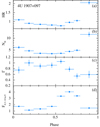 |
Fig. 1. Swift/XRT hardness ratio of 4U 1907+09, and best-fit parameters as a function of orbital phase (absorption column density NH in units of 1022 cm−2, power-law photon index Γ, and 0.3–10 keV flux not corrected for absorption in units of 10−10 erg cm−2 s−1). |
We also provide the first detailed analysis of an XMM-Newton observation that was previously reported by Giménez-García et al. (2015) extracting only the average spectrum for a study aimed primarily at the iron line emission. XMM-Newton observed 4U 1907+09 close to the epoch of periastron passage from 2009-04-18 at 12:16:25 to 2009-04-18 at 18:08:50 UT (OBSID 0555410101) for a total exposure time of about 20 ks. The EPIC-pn and MOS1 cameras were operated in timing mode, while the MOS2 in small-window mode. The observation was not affected by any flaring background time interval, and thus we retained the full observation exposure for the scientific analysis.
We extracted the EPIC-pn events in a region encompassing 80% of the source net signal (from RAWX 27 to 45 inclusive) and a background region with a width of 15 RAWX units (RAWX 7–22). We extracted the MOS1 source events in a circular region with a radius of 800 pixels, centered at the source best position, while we chose a background region with a radius of 1200 pixels in an external CCD. We extracted the MOS2 source events encompassing 80% of the source net signal (RAWX 290–318 inclusive) and a background box 2400 × 9600 pixels in size located on an external CCD, unaffected by the source signal.
We found a satisfactory fit to the source averaged EPIC-pn, MOS1, and MOS2 spectra using an absorbed power-law model (we adopted the TBABS component as for Swift/XRT) and a partial covering (PCFABS in XSPEC). We also found clear evidence of a prominent iron line at ∼6.4 keV that was modeled in the fit using a Gaussian line with zero width. Due to the known calibration limitations for the different operating modes of the EPIC cameras, we restricted the fit to the energy range 1.1–10 keV for EPIC-pn, 0.5–10 keV for MOS1, and 0.5–1.1 keV plus 1.8–10 keV for MOS2. Even though these choices exclude the obvious residuals linked to calibration uncertainties, scattered points remained visible, especially below ∼2 keV (see Fig. 2). We added a 2% systematic error on the spectrum to obtain a fit acceptable at the 4σ level, as the scattered residuals did not suggest the presence of an additional spectral component (χ2 = 466 for 352 degrees of freedom, hereafter d.o.f.)4. The best-fit parameters are reported in Table 2. Here and in the following, NH is the absorption column density along the direction to the source (including the Galactic absorption), NH, pc is the column density of the partial absorber (representing the absorption column density local to the source), f is the covering fraction of the partial absorber, Γ is the power-law photon index, EFe and normFe are the centroid energy and normalization of the Gaussian line representing the iron emission, and F2 − 10 keV is the measured 2–10 keV power-law flux in units of 10−12 erg s−1 cm−2. Based on the current knowledge of the EPIC cameras calibrations, we consider the 7% difference in the MOS1 instrument normalization within the expected systematic calibration uncertainties of the different modes.
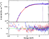 |
Fig. 2. 4U 1907+09 unfolded spectra obtained by using the entire exposure time available in the XMM-Newton OBSID 0555410101 for the EPIC-pn (black points), MOS1 (red crosses), and MOS2 (blue circles) cameras. The residuals from the best-fit model are reported in the bottom panel. |
Best-fit parameters obtained from the XMM-Newton data of 4U 1907+09 collected during the observation 0555410101.
From the cleaned EPIC-pn source event file list, we determined the best source spin period using the epoch-folding technique (see, e.g., D’Aì et al. 2011) at 2.2631(7) mHz and then extracted the background-subtracted energy-resolved light curves of the source in the 0.5–3 keV and 3–10 keV for all EPIC cameras binned at the above period, such that any variability observed can be ascribed to the accretion environment and not the energy dependence of the source pulse period. The hardness ratio obtained after combining EPIC-pn, MOS1, and MOS2 data is shown in panel a of Fig. 3, while the corresponding count rate is given in panel b. The source displays a remarkable variability, with the largest changes in the HR visible toward the end of the observation, when the source enters a lower X-ray emission state.
 |
Fig. 3. Timing analysis of 4U 1907+09. Top left, panel a: hardness ratio of the combined EPIC-pn, MOS1, MOS2 light curves (3–10 keV/0.5–3 keV). Top left, panel b: total rate in the 0.5–10 keV energy range. Bottom left, panel c: distance dj from the average for each pulse profile as function of HR. Bottom left, panel d: distance dj from the average for each pulse profile as function of the total rate. The numbers indicate the different intervals identified in panel b (see Eq. (1) for the definition of dj). Right: plot of the best-fit parameters as a function of time obtained from the HR-resolved spectral analysis of the XMM-Newton observation of 4U 1907+09. The parameters reported in the different panels are those introduced in Table 2 and described in the text. |
We highlight as red vertical lines in panels a and b of Fig. 3 the time intervals with significant variations of the HR in which we extracted spectra to investigate the possible origin of this variability. We show the best-fit spectral parameters as function of time in Fig. 3. The centroid energy of the iron line is not shown because it remained stable at the value measured from the average spectrum to within the associated uncertainties. For each time interval, the EPIC-pn, MOS1, and MOS2 spectra were extracted and fit together with the same model used for the averaged spectrum (see earlier in this section). We note that fixing the value of the TBABS absorption column did not result in acceptable fits for all spectra so we left this parameter free to vary, also for the HR-resolved spectral analysis. It is evident from this figure that the time intervals during which the higher HR has been recorded are characterized by an overall enhanced local absorption column density (NH, pc), while the covering fraction remains relatively stable around the average value and the power-law photon index displays only a modest softening compared to the initial part of the observation. Interestingly, the lowest values of the absorption column density are measured close to the peaks of the brightest emission episodes. We verified that the hardness is driven mainly by the variation in the column density in the partial-covering component by checking the linear correlation between HR and NH, pc that is significant at 99% confidence level using the r2 statistics on a sample of 1000 bootstrapped data sets, distributed according to the actual measurements. Other parameters are not significantly correlated to the HR. We also investigated the correlations between spectral parameters, but could not find any significant linear trend.
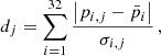
For each time interval of different hardness ratio in panels a and b of Fig. 3, we folded the total light curve at the NS spin period to extract the pulse profiles. In Fig. 4, we show the pulse profiles after dividing them for their average and displacing them vertically by ten times their distance from the average profile, computed as
 (1)
(1)
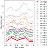 |
Fig. 4. Average and HR-resolved pulse profiles of 4U 1907+09 divided by their mean and vertically displaced by ten times their distance from the average, as computed in Eq. (1). The symbols represent the pulse profile as labeled in panel a of Fig. 3. |
where j represents the pulse-profile number, pi, j is the i-th bin of the j-th pulse profile, σi, j is the uncertainty, and  is the average i-th bin of the average pulse profile. The label of each line represents the number of interval j from 0 to 17, as indicated in panel b of Fig. 3. In this figure, we also show for each HR interval the pulse variability as function of the HR (panel c) and of the total rate (panel d).
The time intervals in which the source is brighter are characterized by pulse profiles that are more similar to the average profile. However, we note a pronounced variation in the shape of the pulse profile, compared to the average shape, during the lower luminosity HR intervals. The most peculiarly shaped pulse profiles are recorded during HR intervals 6–8, immediately following the brightest source emission phase toward the middle of the XMM-Newton observation. Intervals 13–15 are instead characterized by the highest HR values (and average fluxes), but the corresponding pulse profiles are quite similar to the average profile. Interval 11 has one of the highest recorded HR values, a relatively low flux, and is characterized by a shape of the pulse profile with intermediate properties between the average profile and those of the most peculiar intervals 6–8.
3.1.2. Discussion of the results
The Swift/XRT orbital monitoring of the source provided some interesting results. As shown in Fig. 1, the flux is remarkably peaked around phase 0.5–0.8, remaining virtually constant during the rest of the orbit. The source also displays a strongly variable absorption column density and photon index along the orbital phase. In particular, the evident spectral hardening around phase 0.8–1.0 is driven by both an increase by a factor of ∼2 in the local absorption column density and a flattening of the spectral index. As phase 0 in our calculation was assumed to be the same as that of in ’t Zand et al. (1998), this point corresponds to the epoch of the mean longitude 90°, that is when the NS is beyond the companion right along the line of sight to the observer. This occurs slightly after the periastron passage that corresponds to phase ∼0.7. Compatible results were obtained in the past by using ASCA and RXTE data (Roberts et al. 2001; Şahiner et al. 2012), although the monitoring presented here with XRT provides an extension of the coverage at the softer X-rays (down to 0.3 keV) and the orbital-phase-resolved spectral analysis is carried out by averaging multiple observations over several orbital cycles rather than making use of single short pointings (a few kiloseconds) carried out at specific orbital phases within the same orbital revolution.
The flux increase close to periastron passage is to be expected in a moderately eccentric wind-fed SgXB, especially if the photoionization of the stellar wind by the accreting NS is relatively low. This is due to the higher density of a line-driven wind closer to the supergiant star, as well as the decrease in the relative velocity between the NS and the companion’s wind, both effects leading to an enhanced mass accretion rate onto the compact object (see, e.g., Bozzo et al. 2021, and references therein). The interpretation of the spectral hardening around phase 0.8–1.0 is less straightforward, and was largely debated also in the past (see Roberts et al. 2001, and references therein). The most widely accepted explanation is the presence of a trailing gas stream connecting the supergiant with the NS, similarly to what was considered to explain the case of the eccentric HMXB GX 301−2 (Leahy 1991; Leahy & Kostka 2008; Kostka & Leahy 2010). Although the statistics of the XRT data do not allow us to establish a firm conclusion, our findings are fully consistent with those reported in the past. Future observations carried out with grating instruments (such as those on board XMM-Newton and Chandra) might be exploited to further corroborate this scenario looking for changing photoionization lines as a function of the orbital phase, as was done in the case of the SgXB Vela X-1 (Watanabe et al. 2006).
The pointed XMM-Newton observation of 4U 1907+09 allowed us to study the variability of the source emission over short timescales, typical of the wind accretion process (see Sect. 1). Once the XMM-Newton light curve is binned at multiples of the best-determined spin period, the observed variability can be ascribed to changes in the accretion environment surrounding the compact object, and as noted in Fig. 3, the highest recorded values of the local absorption column density occur during periods when the source intensity is low. A similar behavior has been observed in other SgXBs and commonly ascribed to the presence of massive clumps passing occasionally in front of the NS along the line of sight to the observer without being accreted, and thus without producing an enhanced X-ray emission. The HR-resolved spectral analysis reported in Fig. 3 supports this conclusion because it shows that NH, pc is the main driver of spectral variability during the second half of the observation. From the same figure, we also observe that there is a decrease in the local absorption column density around the peaks of the flares taking place during the first ∼10 ks of the observation and that there are two sharp decreases in the covering fraction at the beginning of the observation (before the bright flares go off) and right after the end of the flaring period. Drops in the local absorption column density during the brightest emission periods are usually interpreted as being due to the photoionization of the clumpy stellar wind by the X-rays from the compact object, while the initial low value of the covering fraction could indicate that there was a progressive fragmentation of a dense clump before the flaring period began. The recorded drop in the covering fraction after the flare could be explained in this context as the residual (non-accreted) portion of the fragmented dense clump moving away from the compact object (see, e.g., Bozzo et al. 2011, and discussions therein).
The average source pulse profile, mediated using the entire exposure time available of the XMM-Newton observation shows a spin-phase variability virtually identical to what has been reported previously (see, e.g., in ’t Zand et al. 1998). A study of the variability of the pulse profile with the source intensity, to the best of our knowledge, was attempted in the past by Roberts et al. (2001) using four different ASCA observations (see also Mukerjee et al. 2001; Fritz et al. 2006; Rivers et al. 2010). These data spanned a total range in the source X-ray luminosity of a factor of ∼60 and highlighted some possible changes in the pulse profile shape as a function of the intensity, but the signal was too low to perform any meaningful comparison among the different profiles. As shown in Figs. 4 and 3, the relatively high statistics and uninterrupted exposure of the XMM-Newton observations allowed us to report here for the first time an analysis of the pulse profile resolved in intensity and HR. We found that the shape of the pulse profile displays a remarkable variability compared to the average profile, with the largest deviations being recorded during the intervals 6, 7, and 8 (see panel d of Fig. 3). These intervals correspond to a period of relatively faint emission from the source (combined count rate from the EPIC cameras of ≲30 cts s−1) and immediately precedes the burst of two faint flares from the source, during (and after) which the highest HR values are measured (see panels a and b of Fig. 3). As our HR-resolved spectral analysis demonstrated that the HR variations are driven by the increase in the local column density and since changes in the shape of the pulse profile in HMXBs are known to be associated with switching between different accretion geometries (see Parmar et al. 1989, for an early discussion), we infer that the encounter of a stellar wind clump with a NS can sometimes alter the way in which the material is accreted and not only the mass accretion rate or the absorption. However, the two phenomena are not necessarily connected. Although this is a somewhat standard assumption in theoretical models proposed to interpret wind-fed systems (see, e.g., Bozzo et al. 2008; Shakura et al. 2012, and references therein), we are not aware of other similar evidence in SgXBs. This result could only be obtained by combining the HR-resolved spectral analysis with a HR-resolved study of the source pulse profile, a technique that our group plans now to exploit for additional bright sources within the SgXB class.
It is worth mentioning here that additional evidence in favor of the scenario proposed above could be obtained by performing a pulse-phase-resolved spectral analysis of the source emission within each identified HR time interval in Fig. 3 (panels a and b). Unfortunately, the statistics of the XMM-Newton data are not sufficient to carry out such an analysis (only one single EPIC spectrum can be extracted for each HR time bin in order to achieve a meaningful spectral fit). This limitation cannot be overcome by using deeper observations with any currently available facility as the required statistics are limited by the X-ray photons collection capability of the existing instruments. This is directly related to the available effective area of the instrument, and under this respect the XMM-Newton EPIC cameras are already providing the best performance. Future instrumentation endowed with a much larger area in the soft X-ray domain, such as the XIFU and WFI on board Athena (Barret et al. 2016; Meidinger et al. 2015) or the LAD on board the eXTP (Zhang et al. 2016) or the STROBE-X (Ray et al. 2019) missions, could provide the necessary advancements to reveal the nature of the pulse profile changes in 4U 1907+09 and other wind-fed systems.
3.2. IGR J19140+0951
IGR J19140+0951 was discovered by INTEGRAL in 2003 (Hannikainen et al. 2004) and later classified as a classical SgXB thanks to the identification of the optical counterpart as a B0.5 Ia star (Torrejón et al. 2010) and the detection of an orbital period of 13.5 d (see, e.g., Wen et al. 2006, and references therein). The distance to the B0.5 Ia star has been recently determined using Gaia data from the originally estimated 3.6 kpc (Torrejón et al. 2010) to 2.8 (Arnason et al. 2021). Sidoli et al. (2016) reported about the discovery of a possible pulsation period from a Chandra observation of the source at ∼5937 s and a quasi-periodic oscillation (QPO) from an XMM-Newton observation of the source at a frequency of ∼1.46 mHz. The QPO has been interpreted as being due to the onset of a quasi-spherical accretion regime.
3.2.1. Data analysis and results
Our Swift/XRT monitoring campaign on IGR J19140+0951 was carried out in 2015 at a pace of two observations per week, each 1 ks long, spanning from February to September 2015 (OBSID 30393). These observations (see Table C.2), for a total exposure of ∼60 ks, cover a bit less than 17 revolutions of the system. The log of the XRT observations in the table also shows for each XRT observation the orbital phase according to the ephemerides reported in Table 1. We note that as the previous ephemerides of the source were published by Corbet et al. (2004) using RXTE/ASM data up to 2004 and since then an additional 8 years of ASM data plus about 15 years of Swift/BAT monitoring data on the source have been made available, we were able to refine the determination of the orbital period to the value reported in Table 1 (all analysis details are provided in Appendix A). We also note that in the case of IGR J19140+0951 the spin period is not known and the tentatively reported period by Sidoli et al. (2016) is far too long to allow any meaningful search in the short XRT observations.
The plot of the source HR as a function of the orbital phase is shown in Fig. 5a. We fit the eight spectra extracted from the eight phase bins with an absorbed power law, and report the results in Table 3 and Fig. 5 (panels b–d).
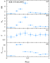 |
Fig. 5. Same as Fig. 1, but for IGR J19140+0951. Here the flux is given in units of 10−11 erg cm−2 s−1. |
Results of the orbital-phase-resolved spectral analysis conducted on the Swift/XRT observations of IGR J19140+0951.
For completeness, we mention here that the sole XMM-Newton observation of the source published by Sidoli et al. (2016) does not allow any HR-resolved spectral investigation as the source was relatively faint during the time spanned by the XMM-Newton data and no flare was apparent from the source light curve (see Fig. 3 in Sidoli et al. 2016).
3.2.2. Discussion of the results
The plot of the spectral parameters and HR as a function of the orbital phase (Fig. 5) obtained from the XRT monitoring of the source displays a rather intriguing variability with the peak of the X-ray flux measured at phase 0.2–0.4, which is consistent with the sharply peaked average orbital profile obtained in the 15–50 keV band using 15 years of continuous monitoring by Swift/BAT (Fig. A.1). We find a steep increase in the absorption column density immediately following and reaching the maximum at phase 0.4–0.5. A similar increase in the source local absorption column density at specific orbital phases was already reported by Prat et al. (2008). However, their measurements as a function of the orbital phase were affected by large uncertainties mainly due to the limited coverage below 3 keV. Our results show that the orbital variability of the flux and absorption column density in IGR J19140+0951 is much more extreme than what was observed before, and it is remarkably similar to what is observed from the much better studied source 4U 1907+09. In both systems there is a shift in phase of about ∼0.2 between the maximum of the flux and the maximum of the absorption column density, and the profile of the flux variability is also peaked at a restricted interval in the orbital phase (≲0.2). In both sources there is also a relatively modest to no change in the power-law slope. We thus conclude that the same scenario that has been proposed for 4U 1907+09 is, most likely, also applicable to the case of IGR J19140+0951; this source will probably be characterized by a non-negligible eccentricity and there should be a large structure located close to the NS and moving with the compact object, possibly a gas stream as indirectly proved in the case of 4U 1907+09. Although we cannot firmly exclude alternative scenarios, the data so far are compatible with this hypothesis, and the similarity with the case of 4U 1907+09 provides support in the right direction.
A measurement of the eccentricity in the case of IGR J19140+0951 would be best obtained by following the evolution of the source spin period at different orbital phases. However, the possibly long spin period of the source (over 5 ks, to be confirmed, see Table 1) would make such measurements extremely time consuming for any sufficiently sensitive facility capable of performing uninterrupted observations of several tens of kiloseconds (e.g., the EPIC cameras on board XMM-Newton). A validation of our proposed scenario for IGR J19140+0951 through the direct comparison with 4U 1907+09 could be obtained by also exploiting deep X-ray observations of the source at specific orbital phases, especially around the peak of the absorption column density where emission or absorption lines can provide a measurement of the ionization status of the absorbing material and its position compared to both the NS and the supergiant companion.
3.3. IGR J11215−5952
IGR J11215−5952 is the only SFXT source displaying regular outburst at the periastron passage and having a well-measured spin and orbital periods. The systems hosts a ∼187 s spinning NS orbiting every ∼165 days around the B0.5 Ia companion, located at a distance of 6.5 kpc (see Sidoli et al. 2020; Arnason et al. 2021, and references therein). The source has been observed many times with virtually all available X-ray facilities and the regularity of its luminosity variations allowed the scheduling of targeted X-ray observations right at the peak of the brightest emission periods. These observing campaigns were aimed at obtaining high S/N data and looking for CRSFs, but to date no firm detection has been reported (Sidoli et al. 2017, 2020). The role of clumps in the accretion process this system is undergoing is of wide interest because the supergiant star in IGR J11215−5952 shows evidence of a magnetized stellar wind and, when this magnetic field is carried by the clumps, it can lead to reconnections and subsequent bright episodes of X-ray emission. This mechanism is one of the proposed scenarios to interpret the peculiar behavior of the SFXTs in X-rays (Hubrig et al. 2018).
3.3.1. Data analysis and results
We report on a new XMM-Newton observation of the source performed from 2021-01-25 at 23:32:04 to 2021-01-26 at 05:01:25 (OBSID 0862410301). Out of the 19.8 ks of EPIC-pn exposure, we retained 15.6 ks after removing periods of background flaring. For the EPIC-pn we use a source extraction region with radius on 0.53 arcmin, based on the radius at which the surface brightness of the source equals the surrounding background and an adjacent background region with radius of 1 arcmin. For MOS1 we use a source extraction region fixed to lie within the small windows of 0.47 arcmin and a background region with radius 1 arcmin in an external CCD. For MOS2, we used RAWX from 282 and 322 for the source, which encompasses 60% of the PSF, to avoid the contribution from a field source, and a background region with the shape of a box 8 × 2 arcmin.
We extracted light curves in the 0.5–3.5 and 3.5–10 keV bands to compute the HR. We caught the source in an episode of decreasing flux characterized by a softening spectrum (see Fig. 6). We managed to describe both the average and HR-resolved spectra using a power law modified by full neutral absorption (TBABS) and a partial covering component (PCFABS). The best C-stat is 238, compared to 295 obtained using an absorbed power law. To test the significance of the improvement, we simulated, for each best-fit model, 100 spectra with equivalent exposure and background using parameters extracted from the chain used to compute uncertainties. For each simulated spectrum, we performed a fit with the same model. For the absorbed power law, 20% of the simulated spectra have a higher C-stat than the real spectrum, while adding a partial covering component this fraction increases to 93%, indicating a significant improvement. As can be appreciated in Fig. 6, the parameter showing the strongest variability is the power-law photon index, suggesting that the softening is mostly linked to intrinsic change in the emission rather than to intervening absorption. We investigated the parameter linear correlations, but the small number of available points prevents any significant detection.
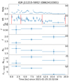 |
Fig. 6. Plot of light curve, HR, and best-fit parameters as a function of time obtained from the HR-resolved spectral analysis of the XMM-Newton observation of IGR J11215−5952. Panel a: source count rate in the 0.5–10 keV bands, after adaptive rebinning with minimum S/N of 15 in the light curve extracted for 0.5–3 keV; panel b: HR between the 3–10 keV and 0.5–3 keV energy-resolved light curves with the identified time intervals for the spectral extraction (red lines); panel c: f, covering fraction of the partial absorber; panel d: Γ, power-law photon index; panel e: NH, absorption column density along the direction to the source (including Galactic absorption); panel f: NH, pc, absorption column density of the partial absorber (representing the absorption column density local to the source; PCFABS in XSPEC); panel g: F2 − 10 keV, measured power-law flux in the 2–10 keV energy range not corrected for absorption for the EPIC-pn in units of 10−12 erg s−1 cm−2. |
3.3.2. Discussion of the results
During the new XMM-Newton observation, IGR J11215−5952 displayed a progressively fading light curve with a single weak flare occurring at t ∼ 2 ks and lasting only a few hundred seconds (see Fig. 6). The flare was far too faint to detect any significant HR variation. There is an intriguing dip in the X-ray emission visible 7.5 ks after the beginning of the observation, but the count rate was too low to detect any HR variability within the dip itself. As summarized in Fig. 6, our Bayesian analysis technique identified three different time intervals with a decreasing trend in the overall HR. This trend seems to be mostly driven by a softening of the power-law photon index, although the error bars associated with the best-fit parameters in all intervals are relatively large due to the limited statistics of the data. The significant detection of a partial covering component in the spectrum of the source is consistent with the clumpy wind accretion scenario (see Sect. 1), although confirmation through the detection of spectral variability along the rise and decay of brighter flares–outbursts would help us strengthen this conclusion.
3.4. IGR J18410−0535
IGR J18410−0535 was discovered by ASCA in 1994 (AX J1841.0-0536; see Bamba et al. 2001) and was associated with the class of the SFXT thanks to the discovery of repeated bright sporadic outbursts by INTEGRAL (Rodriguez et al. 2004; Sguera et al. 2006; Walter & Zurita Heras 2007). The optical counterpart was identified as a B1 Ib supergiant at roughly 3.2 kpc (Nespoli et al. 2008). Although the system is thought to host a NS, neither the compact-object pulse period nor the binary orbital period has been firmly measured. During a bright flare caught by XMM-Newton in 2011, the source displayed the clearest observational evidence to date in favor of clumpy winds playing a major role in the X-ray variability of SgXBs (Bozzo et al. 2011). In 2019 an XMM-Newton observation caught the source in the faintest observed state with an upper limit of 2 × 10⁻¹⁴ erg s−1 cm−2 at 90% confidence level in the 1–10 keV energy band (Ferrigno et al. 2020).
3.4.1. Data analysis and results
Here, we report on a snapshot that XMM-Newton performed on IGR J18410−0535 from 2020-10-17 at 20:00:11 to 2020-10-18 at 02:23:31 UT (OBSID 0862410101). The EPIC-pn was operated in full frame, the MOS1 in small window, and the MOS2 in timing mode. The observation was marginally affected by flaring background, so we retained a good time of 14.6 ks out of an elapsed time of 15 ks. The source had an average count rate of 0.4 cts s−1 in the EPIC-pn 0.5–10 keV band and did not show any appreciable variation in hardness ratio (Fig. 7). We model the average spectrum extracted from the three cameras with an absorbed power law with best-fit parameters reported in Table 4.
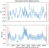 |
Fig. 7. Timing analysis of the of the 2020 observation of IGR J18410−0535 (OBSID 0862410101). Lower panel: combined EPIC-pn+MOS1+MOS2 light curve in 0.5–10 keV energy range. Upper panel: hardness ratio between the light curves in the bands 3.5–10 keV and 0.5–3.5 keV rebinned at a minimum S/N of 8. There are no significant variations in the hardness ratio, and thus the Bayesian algorithm identified a single time interval for the spectral extraction (red lines, corresponding to the whole observation). |
Best-fit parameters of the XMM-Newton observation of IGR J18410−0535 carried out in 2020 (OBSID 0862410101).
3.4.2. Discussion of the results
Although IGR J18410−0535 is one of the best known SFXTs to have shown the clearest evidence of clumpy wind accretion due to a bright outburst in 2011 (Bozzo et al. 2011), our targeted XMM-Newton observations to the source were not able to catch additional bright events. Following the deep upper limit on the source flux that we obtained with an observation in 2019, during the additional pointing in 2020 we could only detect a moderately faint flare in the EPIC light curves (see Fig. 7). During the rise and decay of this flare, and during the remaining part of the XMM-Newton observation, we did not record any significant variation in the HR that could have indicated a change in the spectral parameters and thus provide evidence in favor of clumpy wind accretion during the low emission state of the source. Given the peculiarity of the 2011 bright outburst, the source clearly deserves further attention, and more flares at intermediate luminosity between outburst and quiescence are needed to complete our investigation of the clumpy wind accretion in this source.
3.5. IGR J16393−4643
IGR J16393−4643 is a classical SgXB discovered by INTEGRAL in 2004 (Bird et al. 2004) and associated with the previously known X-ray source AX J1639.0-4642 (Sugizaki et al. 2001). The system hosts a ∼910 s spinning NS (Bodaghee et al. 2006) orbiting around a still poorly known OB companion, and the measured orbital period is of ∼4.24 d (see Corbet & Krimm 2013, and references therein). The usually heavy extinction measured from X-ray observations in the direction of the source led to the inclusion of this system within the highly obscured X-ray pulsars, a class of objects that has been largely revealed thanks to INTEGRAL observations (see, e.g., Walter et al. 2015, and references therein). IGR J16393−4643 has also shown evidence of a super-orbital modulation, although no firm conclusion has been reached yet (Corbet et al. 2021). The discovery of a CRSF at ∼29.3 keV led to the determination of the NS magnetic field strength at 2.5 × 10¹² G (Bodaghee et al. 2016).
3.5.1. Data analysis and results
Our monitoring campaign of IGR J16393−4643 was carried out in 2016 with Swift/XRT from January to June 2016, at a pace of one observation of 1 ks per day (OBSID 34135, for a total of 130 ks), thus covering slightly more than 31 revolutions of the system. A selection of these data (∼70 ks) have been reported by Kabiraj et al. (2020). These authors focused on the properties of the suspected source X-ray eclipse and suggested that this might not be a true eclipse, although it regularly occurs at the same orbital phase. Here we reanalyze the whole data set to carry out an orbital-phase-dependent HR-resolved spectral analysis with the main goal of identifying spectral changes that could point toward the existence of large-scale structures in the stellar wind around the compact object.
The Swift observing logs for IGR J16393−4643 are reported in Table C.3, where we also indicated the orbital phase estimated for each observation by adopting the same ephemerides as in Kabiraj et al. (2020, see Table 1). The equivalent of Fig. 1 but realized in the case of IGR J16393−4643 is shown in Fig. 8a.
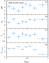 |
Fig. 8. Same as Fig. 1, but for IGR J16393−4643. Here the flux is given in units of 10−11 erg cm−2 s−1. |
In order to investigate possible spectral variability in different orbital phase bins, we extracted different source spectra for each of these bins and fit them by using a simple absorbed power-law model. The results are shown in Table 5 and Fig. 8 (panels b–d).
Results of the orbital-phase-resolved spectral analysis conducted on the Swift/XRT data of IGR J16393−4643.
We also checked in the XMM-Newton archive suitable observations of IGR J16393−4643 to carry out a HR-resolved spectral analysis aimed at discovering possible spectral variability. The source was observed twice by XMM-Newton in 2004 and in 2010. However, neither observation is suitable for our goal. The observation in 2004 is relatively short (∼8 ks) and it shows eight peaks and valleys corresponding to the source pulse period (Bodaghee et al. 2006). There is no flaring behavior that could be analyzed to look for HR variations. During the slightly longer observation carried out in 2010 (∼10 ks), the source was a factor of ≳10 fainter and the light curve does not show any flaring behavior that is bright enough to carry out a meaningful HR-resolved spectral analysis (see also Pradhan et al. 2018).
3.5.2. Discussion of the results
Our detailed study of the source orbital-phase-resolved HR and spectral properties extends and completes the previous work from Kabiraj et al. (2020). We analyzed all XRT data of our monitoring campaign with a uniform technique exploited for all the SgXBs in this paper (to facilitate a direct comparison) and computed the HR value of the folded XRT data over the source orbital period in eight phase bins containing the same number of photons. The spectra extracted in each of these bins could be well fit with a simple absorbed power-law model, and the plot of these parameters (as well as the HR) as a function of the orbital phase in Fig. 8 does not show any prominent variability. There is a potentially interesting V-shaped feature in the profile of the source flux between phases 0.3–0.5, but this feature does not seem to be connected with either a significant change in the power-law slope or a variation in the local column density. The source is heavily obscured along the entire orbit (NH ≫ 1023 cm−2) and the limited band-pass of the XRT energy coverage did not reveal significant variations of the HR (given also the relatively large associated error bars).
The relatively sharp drop in the source X-ray flux around phase 0.75–1.0 corresponds to the suspected eclipse studied also by Kabiraj et al. (2020) and Islam et al. (2015). In agreement with their results, our analysis also suggests that, despite the decrease of a factor of ≳2 in the source flux, the other spectral parameters did not show at this particular orbital phase a dramatic variation compared to other phases. We recorded a flattening of the power-law photon index that, in principle, is expected in case of an X-ray eclipse. However, this is not accompanied by a drop in the local absorption column density. This drop is expected because during the eclipse the source of the X-rays is hidden from the direct view of the observer who is looking instead to the remaining diffuse fluorescence emission of the X-rays from the occulted NS onto the surrounding wind material spread all around the binary system (see, e.g., Bozzo et al. 2009, and references therein).
The XRT data are thus raising concerns against the interpretation of the drop in flux at phases 0.75–1.0 as an X-ray eclipse, but the statistics are far too low to allow a deeper analysis. Kabiraj et al. (2020) proposed that this drop in flux could be caused by a grazing eclipse and absorption of the X-rays in the stellar corona. At present, however, alternative possibilities cannot be excluded. In the context of the corotating interaction regions there could be the intriguing possibility that the obscuration is due to one of these large structures that is tilted away from the plane of the NS orbit and that it attenuates the X-ray emission along the line of sight to the observer mainly through scattering with a non-measurable enhancement of photoelectric absorption like that for the grazing eclipse (an idea put forward in Bozzo et al. 2016). Interestingly, the source has also displayed evidence for an at least transitory super-orbital period, whose origin could also be related to corotating interaction regions (Corbet et al. 2021). The peculiar orbital phase 0.75–1.0 of IGR J16393−4643 deserves a dedicated observation with larger effective area instruments (such as the EPIC cameras on board XMM-Newton) able to detect any emission or absorption lines, providing details about the physical conditions of the material causing obscuration, and to reveal modest variations in the spectral parameters that could go undetected due to the limited statistics of the Swift/XRT data.
3.6. XTE J1855−026
XTE J1855−026 was discovered by the RXTE satellite in 1998 (Corbet et al. 1999) and it is known to host a ∼361 s spinning NS, orbiting every 6.1 d a BN0.2 Ia supergiant star located at roughly 10 kpc (see González-Galán 2015, and references therein). The optical companion was identified thanks to the refined Swift position obtained with an arcsec level accuracy (Romano et al. 2008). XTE J1855−026 is known to be eclipsing (see Falanga et al. 2015; Coley et al. 2015, for the most updated source ephemerides) and it has long been classified as a classical SgXB, although its behavior is partly anomalous compared to other objects of this class due to the emission of sporadic bright X-ray outbursts. These have been observed a few times with INTEGRAL and Swift (see, e.g., Watanabe et al. 2010; Krimm et al. 2012, and references therein).
3.6.1. Data analysis and results
We report on a detailed analysis of the as-yet-unpublished Swift data (see Table C.4) collected during the outburst observed in 2011 (Krimm et al. 2012). This is the only outburst for which data in the soft X-ray domain (≲1–2 keV) are available.
XTE J1855−026 triggered the BAT (image trigger 503434) on 2011 September 18 at 10:07:28.6 UT (T0, MJD 55822.42186, orbital phase 0.61); Swift slewed to the target so that the narrow-field instruments started observing at T0+1510 s (see Table C.4). The BAT event data were analyzed using the standard BAT analysis software within FTOOLS. Mask-tagged BAT light curves, covering the time range T0 − 239 to T0 + 963 s, were created in the standard energy bands (15–25, 25–50, 50–100, 100–350 keV), and rebinned to fulfill at least one of the following conditions: reaching a signal-to-noise ratio (S/N) of 5 or a bin length of 10 s. The light curves of the first orbit of data are shown in Fig. 9. A mask-weighted spectrum was also extracted from the events collected during the first orbit; we applied an energy-dependent systematic error vector to the data and created response matrices with BATDRMGEN using the latest spectral redistribution matrices. This spectrum, when fit in the energy range 15–70 keV with a simple power law, yields a photon index of 2.48 ± 0.15 (χ2/d.o.f. = 30.90/24) and a 15–50 keV flux of (2.27 ± 0.08)×10−9 erg cm−2 s−1 (see Table 6). This fit, however, shows residuals that indicate a curvature, so a fit with a cut-off power-law model was also made, yielding a photon index of  and a cut-off energy E
 keV (χ2/d.o.f. = 16/23). We note that there are no XRT data simultaneous with this BAT spectrum.
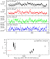 |
Fig. 9. Light curves of the 2011 September 18 outburst of XTE J1855−026 caught by BAT and XRT. Panels a–d: BAT light curves (c s−1, at 10 s binning); panel e: XRT light curve (0.3–10 keV c s−1); the horizontal red line indicates the time where the BAT event data were collected. A different scale is used for the x-axis. |
Spectral analysis conducted on the Swift observations of XTE J1855−026.
The XRT light curve, split into three snapshots, starts at T0 + 1510 s and shows a dynamic range of ∼20 in ∼6 ks (0.3–10 keV, see Fig. 9). The hardness ratio calculated in the 0.3–4 and 4–10 keV bands is shown in Fig. 10. XRT spectra were extracted in each observing mode and each of the snapshots that comprise the data set, thus obtaining three window timing (WT) and two photon counting (PC) spectra, and were fit with the a simple absorbed power-law model and Cash statistics. A summary of the spectral results is shown in Table 6.
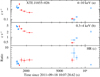 |
Fig. 10. Timing analysis of the XTE J1855−026outburst. Panel a: XRT hard-band light curve (4–10 keV c s−1); panel b: soft-band light curve (0.3–4 keV c s−1); panel c: hardness ratio (4–10 keV/0.3–4 keV). WT data are shown in blue, PC data in red. |
The BAT survey data products, in the form of detector plane histograms (DPHs), are also available, and were analyzed with the standard FTOOLS software. Since BAT survey data are accumulated on board with typical integration times of 300 s, pairing simultaneous BAT survey data with the XRT data is not straightforward. Therefore, we extracted spectra (six energy bins) that most closely matched the XRT data: (i) DPH1 in the time range T0 + 1504–1804 s; (ii) DPH2 in the time range T0 + 1804–2104 s; (iii) DPH3 in the time range T0 + 2104–2382 s. Each BAT spectrum was fit with a simple power-law model (results in Table 6). In order to ensure the closest to simultaneity, we chose to fit the following BAT and XRT groups: (a) DPH1+WT1, (b) DPH2+DPH3+PC2. When fitting these BAT and XRT spectra together, a constant needs to be used to model both the difference of exposure and the non-strict simultaneity. Furthermore, the XRT spectra are fit by minimizing Cash statistics, while the BAT spectra with χ2 statistics.
A fit to the DPH1+WT1 pair with an absorbed power-law model resulted in residuals suggesting a spectral curvature, so we also performed a fit using an absorbed cut-off power law. This yielded a NH = 0.9 ± 0.1 × 1023 cm−2, a photon index of  , and a cut-off energy Ecut = 10 ± 1 keV (inter-calibration constants CDPH1 = 1 fixed and
  ). This is reported in Table 6. The addition of an iron line, represented by a Gaussian model with energy ∼6.4 keV, yields a continuum fit with NH = 0.8 ± 0.1 × 1023 cm−2, a photon index of
  , and a cut-off energy Ecut = 10 ± 1 keV (inter-calibration constants CDPH1 = 1 (fixed) and
  ), while the line is characterized by a centroid energy
  keV and a width consistent with zero (< 1.52 keV) and an equivalent width EW =
  keV (Fig. 11).
 |
Fig. 11. Spectroscopy of the 2011 September 18 outburst of XTE J1855−026. Top panel: unfolded spectra of the nearly simultaneous XRT/WT1 data (blue crosses) and BAT DPH1 data (empty black circles) fit with an absorbed cut-off power-law model. Bottom panel: data/model ratio of the fit. |
Similarly, a fit to the DPH2+DPH3+PC2 group with an absorbed power-law model indicated the presence of a possible spectral curvature in the residuals. An absorbed cut-off power-law fit yielded a NH = 0.6 ± 0.2 × 1023 cm−2, a photon index of  , and a cut-off energy
  keV (inter-calibration constants CSDPH2 = 1 (fixed),
  , and
, and  ). This is reported in Table 6. The addition of an iron line, represented by a Gaussian model with energy ∼6.4 keV, yields a continuum fit with
  cm−2, a photon index of
  , and a cut-off energy
  keV (inter-calibration constants CDPH1 = 1 (fixed) CDPH3 = 1.2 ± 0.1, and and
  ), while the line is characterized by a centroid energy EFe = 6.4 ± 0.2 keV, a width of
  keV, and EW ≫ 1 keV (Fig. 12).
 |
Fig. 12. Spectroscopy of the 2011 September 18 outburst of XTE J1855−026. Top panel: unfolded spectra of the simultaneous XRT/PC1 data (red crosses), the BAT DPH2 data in black (filled circles), and the BAT DPH3 data in gray (empty circles) fit with an absorbed cut-off power-law model. Bottom panel: data/model ratio of the fit. |
3.6.2. Discussion of the results
The outburst of the source in 2011 was the only one where the broadband emission from XTE J1855−026 could be studied combining data from a large field-of-view instrument (Swift/BAT) with those collected in the soft X-rays by a focused telescope (Swift/XRT). Although the XRT light curve during the outburst is fragmented due to the observational strategy of the satellite, the coverage of the outburst allows us to study possible changes in the spectral properties of the source X-ray emission from the onset of the event down to the return to the usual emission level.
We see from Fig. 10 that XRT pointed the source about 1.5 ks after the onset of the outburst. The instrument recorded a progressive rise in the absorption column density, starting at ≲2 × 1022 cm−2 (WT1 and PC1 data in Table 6) and reaching 4 × 1022 cm−2 a few kiloseconds after the beginning of the monitoring (WT2 and PC2 data in Table 6). Interestingly, XRT also recorded a new drop in the absorption column density down to 0.8 × 1022 cm−2 about 11 ks after the onset of the event when the flux decay was interrupted by a new brightening of the source (WT3 data in Table 6). This behavior resembles what is typically observed in clumpy wind accreting systems, but in the case of the 2011 outburst of XTE J1855−026, we likely missed the initial increase in the local absorption column density as the XRT only began observing about 1.5 ks after the onset of the event. Nevertheless, we clearly detect the progressive increase in the local absorption column density during the decay of the outburst associated with the fading of the source and the diminishing effect of the photoionization onto the clumpy wind. The drop in the local absorption column density about 11 ks after the onset of the flare further strengthens this conclusion as it can be ascribed to the renewed effect of the photoionization when the source underwent a second (fainter) brightening.
The onset of the outburst up to 1.5 ks was observed by Swift only with the BAT. The hard X-ray spectrum above 15 keV could be described reasonably well with a simple power law and the measured photon index is compatible with that recorded during the outbursts observed with the hard X-ray imager IBIS/ISGRI on board INTEGRAL (Watanabe et al. 2010). However, the BAT data showed evidence of a possible curvature in the hard energy spectrum, with a cut-off energy at about 16 keV. When the XRT data are combined with the (quasi-)simultaneous BAT survey data during the later stages of the outburst development (data DPH1+WT1 and DPH2,3+PC1 in Table 6), the value of the measured curvature slightly decreases toward ∼10 keV, although the associated uncertainties remained quite large due to the limited statistics of the data. This curvature is almost ubiquitous in accreting SgXBs (see, e.g., Walter et al. 2015, and references therein) and was also reported in the case of XTE J1855−026 (Corbet et al. 1999). In the broadband fit of the XRT+BAT data, we find evidence of the presence of an iron line at a centroid energy of 6.4 keV. Although the statistics of the XRT data in the energy range of the iron line are limited, this feature is expected in the case of a SgXB. The iron line at 6.4 keV is commonly observed in wind-fed systems, due to the fluorescence of the X-rays from the accreting compact object onto the surrounding stellar winds (see, e.g., Torrejón et al. 2010; Giménez-García et al. 2016, for recent reviews). Iron lines with compatible parameters to those measured by XRT were already reported in the case of XTE J1855−026 by Devasia & Paul (2018) using Suzaku data.
Given its classification as a classical SgXB and the presence of peculiar bright short outbursts similar to those of the SFXTs, XTE J1855−026 remains today an intriguing object that has likely not drawn sufficient attention from the community. It remains relatively poorly studied as no detailed orbital monitoring in the soft X-rays has been carried out yet, and we are missing sufficiently long exposure observations with the large-area X-ray instruments (such as the EPIC cameras) to probe possible emission or absorption lines in the high energy domain to investigate the properties of the stellar wind material within the binary. The evidence reported in this paper regarding the clumpy wind accretion in XTE J1855−026 provides good perspectives to renew the interest in this system.
3.7. IGR J17503−2636
IGR J17503−2636 is a SFXT discovered by INTEGRAL in 2018 (Chenevez et al. 2018). The source underwent a bright X-ray flare lasting several hours before rapidly going back to a quiescent emission level (the measured dynamical range in the X-ray domain is ∼300; see Chakrabarty et al. 2018a,b; Ferrigno et al. 2019). The optical counterpart was tentatively identified as a heavily obscured supergiant located beyond the Galactic center (Masetti et al. 2018), although these findings require further consolidation (McCollum et al. 2018). The NuSTAR data collected shortly after the discovery showed evidence of the presence of a cyclotron scattering feature in the broadband spectrum of the source, suggesting that the compact object accreting in this system is a NS endowed with a magnetic field strength of ∼2 × 10¹² G (Ferrigno et al. 2019).
3.7.1. Data analysis and results
We report on our Swift/XRT follow-up campaign until about one year after the discovery of the source, spanning from April to June 2019 (at a pace of one 5 ks observation per week, OBSID 10980), and not yet published elsewhere. As the orbital period of the source is not known, we could only consider here the long-term evolution of the source X-ray emission.
The summary of the available XRT observations of IGR J17503−2636 is provided in Table C.5. In that table we report the measured flux of each XRT observation, together with the best-fit parameters; all spectra of IGR J17503−2636 could be fit well with a simple absorbed power-law model. We also included for completeness in the table one serendipitous ∼2 ks observation in the Swift archive (MJD 56224) preceding the discovery of the source and not published elsewhere. During this pointing, the source was found in a low state (the measured count rate is 5.2 ± 0.7 × 10⁻¹ c s−1 corresponding to a 0.3–10 keV flux of  erg cm−2 s−1). The long-term X-ray light curve of IGR J17503−2636 as measured by XRT is shown in Fig. 13.
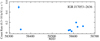 |
Fig. 13. Long-term light curve of IGR J17503−2636 as measured by Swift /XRT. For completeness, we included the XRT observations already published in our previous paper on the source (MJD 58343 and 58333, Ferrigno et al. 2019). |
3.7.2. Discussion of the results
Our XRT monitoring campaign of IGR J17503−2636 demonstrates that the source behaves as most SFXTs do: they remain at a fairly faint quiescent level for most of their lifetime, except for rare and sporadic outbursts (so far only one outburst has been recorded). The source shows a rather stable spectral energy distribution over time during the low-level emission state, as observed in several SFXTs (see, e.g., Walter et al. 2015, and references therein). As the source was regularly detected during each of the performed XRT pointing at a flux of ∼10−11 erg s−1 cm−2 or higher, our campaign seems to invalidate the tentative conclusion presented by Ferrigno et al. (2019), who classify the source as a faint SFXT due to its particularly large distance beyond the Galactic center (proposed to explain why no previous outbursts were ever detected from the source by the large field-of-view instruments on board INTEGRAL and/or Swift).
The measured XRT fluxes correspond to a luminosity of roughly ∼1035 erg s−1 at 10 kpc, and the quiescent luminosity of several SFXTs has been measured to be as low as 1032 erg s−1. The archival XRT observation that we report here for the first time also confirmed that the source was already active at a similar flux level in 2012, about six years before the discovery of the first outburst by INTEGRAL. The reason why no previous outbursts had ever been detected before 2018 remains to be explained. The intrinsic fragmentation of the XRT light curves (due to the pointing strategy of the satellite) also did not allow us to study the SFXT typical behavior of flaring at the lowest emission states, during which evidence of the clumpy wind accretion are commonly found (see Sect. 1). For all these reasons, this source certainly deserves further observations to find clearer evidence of clumpy wind accretion and to measure possible changes in the cyclotron line properties that could be associated with variations in the NS magnetic field configuration.
4. Conclusions
We report in this paper on the outcomes from our concluded observational campaigns of several classical SgXBs and SFXTs with both Swift and XMM-Newton. The goals of our observations were mainly to study structures in the stellar winds surrounding the compact objects in these systems, revealing details of the still highly debated macro-clumps and of other larger structures. In the field of macro-clumping, the results presented here complement those reported in our previous papers, while the longer-term XRT observational campaigns are reported here for the first time.
As a general conclusion, we found that the observational strategies set to study structures in the massive star winds with both XMM-Newton and Swift have been successful so far, with the former focusing on the shorter-term variability (from a few thousand seconds to hours) associated with the accretion of clumps and the latter on the longer-term variability (from a few to several days) associated with different orbital phases of these systems and driven by larger stellar wind structures (such as accretion and photoionization wakes, CIRs, and accretion streams).
Short XMM-Newton observations had been already exploited in a number of previous papers from our group, and although we were able to report in the past on significantly brighter flares than those described here, we could still advance the census of these kind of events from both classical SgXBs and SFXTs. In particular, the observation of the classical SgXB 4U 1907+09 allowed us to provide interesting evidence about how the encounter between the NS and a clump can affect the accretion process beyond the variations of the continuum emission and absorption column density studied before. The lack of spectral variability in the flares recorded from IGR J18410−0535 and IGR J11215−5952 increases the statistics of events that seem to occur without the interventions of clumps, likely triggered by additional mechanisms like centrifugal and magnetic gating or the settling accretion regime. The lack of spectral variability is particularly puzzling in the case of IGR J11215−5952 where the observed flare by XMM-Newton reaches the previously reported threshold of a few cts s−1 above which variations are expected (Bozzo et al. 2017b).
We also exploited in this paper XRT and BAT observations of XTE J1855−026, caught during a rare bright outburst in 2011 (still unpublished). We could study for the first time the source broadband emission with high sensitivity and looked for possible spectral features and variability during the event. Although the source displayed a remarkable dynamic range in its X-ray luminosity, our analysis could not reveal any significant spectral variability. This source is still poorly studied and understood, being characterized by an intermediate behavior between classical SgXBs and SFXTs.
The study of orbital-phase spectral variability reported here for the first time with Swift/XRT has undoubtedly helped us understand which of the observed sources are more likely to display measurable periodic spectral changes along their revolutions. In the case of 4U 1907+09, our XRT campaign confirmed previous findings about the peculiar changes in the source flux, continuum slope, and absorption column density at different orbital phases, but we were able to extend literature studies exploiting the lower-energy band-pass of XRT. This allowed us to reveal even more extreme variations especially of the local absorption column density to the source. Thanks to the XRT coverage at these low energies, we were able to reveal a completely analogous behavior in IGR J19140+0951, and proposed for this object a similar scenario to that studied already in much greater detail for 4U 1907+09, involving the presence of a non-negligible eccentricity and a massive structure moving with the NS, likely a gas stream. Instead, no particularly striking variability has been observed from the orbital monitoring of IGR J16393−4643. This source is relatively faint even for XRT, and although it is possible that some variability has gone undetected within the measured uncertainties of the different spectral parameters, we can definitively rule out prominent spectral changes like those measured from either 4U 1907+09 or IGR J19140+0951. In the case of the SFXT IGR J17503−2636, we could not study spectral variability along the different orbital phases as the system orbital period is not known yet. Our XRT observations revealed, however, that the source remained relatively stable in terms of X-ray flux and spectral energy distribution over time. Having followed the source up to nine months after its initial discovery in 2018 and having reported its detection in an archival XRT observation dating back in 2012, we consider that it is reasonable to assume that the source is displaying a low persistent luminosity with rare outbursts (only one detected so far), as is common for the SFXTs. This further strengthens the previous conclusions about the nature of this source.
The χ2 test statistics are appropriate here as in each spectral bin there are at least 50 counts.
See details in the IBIS/ISGRI data analysis manual at https://www.isdc.unige.ch/integral/analysis.
The documentation is available at https://sextractor.readthedocs.io/en/latest/index.html.
Acknowledgments
The data underlying this article are publicly available from the XMM-Newton, RXTE, Swift, and NuSTAR archives. The full chain of the analysis of the XMM-Newton and INTEGRAL data is available in the form of a python Notebook that can be run in a dockerized environment for 4U J1907+097, IGR J18410−0535, and IGR J11215−5952. We thank the anonymous referee for detailed comments that helped us improve the paper. The Swift data of our monitoring campaigns were obtained through contract ASI-INAF I/004/11/5 (PI P. Romano). PR and EB acknowledge financial contribution from contract ASI-INAF I/037/12/0. This work made use of data supplied by the UK Swift Science Data Centre at the University of Leicester (see Evans et al. 2007, 2009) and by the multi-messenger online data analysis (MMODA) platform at the University of Geneva (see Neronov et al. 2021). CF is grateful to Dr. Volodymyr Savchenko for providing assistance with MMODA and for sharing the tuning of sextractor to the IBIS imaging.
References
- Arnason, R. M., Papei, H., Barmby, P., Bahramian, A., & Gorski, M. D. 2021, MNRAS, 502, 5455 [NASA ADS] [CrossRef] [Google Scholar]
- Bamba, A., Yokogawa, J., Ueno, M., Koyama, K., & Yamauchi, S. 2001, PASJ, 53, 1179 [NASA ADS] [CrossRef] [Google Scholar]
- Barret, D., Lam Trong, T., den Herder, J. W., et al. 2016, in Space Telescopes and Instrumentation 2016: Ultraviolet to Gamma Ray, eds. J. W. A. den Herder, T. Takahashi, & M. Bautz, SPIE Conf. Ser., 9905, 99052F [NASA ADS] [CrossRef] [Google Scholar]
- Bertin, E., & Arnouts, S. 1996, A&AS, 117, 393 [NASA ADS] [CrossRef] [EDP Sciences] [Google Scholar]
- Bird, A. J., Barlow, E. J., Bassani, L., et al. 2004, ApJ, 607, L33 [NASA ADS] [CrossRef] [Google Scholar]
- Bodaghee, A., Walter, R., Zurita Heras, J. A., et al. 2006, A&A, 447, 1027 [NASA ADS] [CrossRef] [EDP Sciences] [Google Scholar]
- Bodaghee, A., Tomsick, J. A., Fornasini, F. M., et al. 2016, ApJ, 823, 146 [NASA ADS] [CrossRef] [Google Scholar]
- Bozzo, E., Falanga, M., & Stella, L. 2008, ApJ, 683, 1031 [Google Scholar]
- Bozzo, E., Stella, L., Israel, G., Falanga, M., & Campana, S. 2009, in Am. Inst. Phys. Conf. Ser., eds. J. Rodriguez, & P. Ferrando, 1126, 319 [Google Scholar]
- Bozzo, E., Stella, L., Ferrigno, C., et al. 2010, A&A, 519, A6 [NASA ADS] [CrossRef] [EDP Sciences] [Google Scholar]
- Bozzo, E., Giunta, A., Cusumano, G., et al. 2011, A&A, 531, A130 [NASA ADS] [CrossRef] [EDP Sciences] [Google Scholar]
- Bozzo, E., Romano, P., Ferrigno, C., Esposito, P., & Mangano, V. 2013a, Adv. Space Res., 51, 1593 [NASA ADS] [CrossRef] [Google Scholar]
- Bozzo, E., Romano, P., Ferrigno, C., et al. 2013b, A&A, 556, A30 [NASA ADS] [CrossRef] [EDP Sciences] [Google Scholar]
- Bozzo, E., Romano, P., Ducci, L., Bernardini, F., & Falanga, M. 2015, Adv. Space Res., 55, 1255 [NASA ADS] [CrossRef] [Google Scholar]
- Bozzo, E., Oskinova, L., Feldmeier, A., & Falanga, M. 2016, A&A, 589, A102 [NASA ADS] [CrossRef] [EDP Sciences] [Google Scholar]
- Bozzo, E., Bernardini, F., Ferrigno, C., et al. 2017a, A&A, 608, A128 [NASA ADS] [CrossRef] [EDP Sciences] [Google Scholar]
- Bozzo, E., Kuulkers, E., Postel, A., et al. 2017b, ATel., 10645 [Google Scholar]
- Bozzo, E., Ducci, L., & Falanga, M. 2021, MNRAS, 501, 2403 [NASA ADS] [CrossRef] [Google Scholar]
- Burrows, D. N., Hill, J. E., Nousek, J. A., et al. 2005, Space Sci. Rev., 120, 165 [Google Scholar]
- Chakrabarty, D., Jonker, P. G., & Markwardt, C. B. 2018a, ATel., 11990, 1 [NASA ADS] [Google Scholar]
- Chakrabarty, D., Jonker, P. G., & Markwardt, C. B. 2018b, ATel., 11991, 1 [NASA ADS] [Google Scholar]
- Chenevez, J., Jaisawal, G., Kuulkers, E., et al. 2018, ATel., 11952, 1 [NASA ADS] [Google Scholar]
- Clavel, M., Tomsick, J. A., Hare, J., et al. 2019, ApJ, 887, 32 [NASA ADS] [CrossRef] [Google Scholar]
- Coley, J. B., Corbet, R. H. D., & Krimm, H. A. 2015, ApJ, 808, 140 [NASA ADS] [CrossRef] [Google Scholar]
- Corbet, R. H. D., & Krimm, H. A. 2013, ApJ, 778, 45 [NASA ADS] [CrossRef] [Google Scholar]
- Corbet, R. H. D., Marshall, F. E., Peele, A. G., & Takeshima, T. 1999, ApJ, 517, 956 [NASA ADS] [CrossRef] [Google Scholar]
- Corbet, R. H. D., Hannikainen, D. C., & Remillard, R. 2004, ATel., 269, 1 [NASA ADS] [Google Scholar]
- Corbet, R. H. D., Markwardt, C. B., & Tueller, J. 2007, ApJ, 655, 458 [NASA ADS] [CrossRef] [Google Scholar]
- Corbet, R. H. D., Coley, J. B., Krimm, H. A., Pottschmidt, K., & Roche, P. 2021, ApJ, 906, 13 [Google Scholar]
- Cox, N. L. J., Kaper, L., & Mokiem, M. R. 2005, A&A, 436, 661 [NASA ADS] [CrossRef] [EDP Sciences] [Google Scholar]
- D’Aì, A., La Parola, V., Cusumano, G., et al. 2011, A&A, 529, A30 [NASA ADS] [CrossRef] [EDP Sciences] [Google Scholar]
- Devasia, J., & Paul, B. 2018, J. Astrophys. Astron., 39, 7 [NASA ADS] [CrossRef] [Google Scholar]
- Doroshenko, V., Santangelo, A., Ducci, L., & Klochkov, D. 2012, A&A, 548, A19 [NASA ADS] [CrossRef] [EDP Sciences] [Google Scholar]
- Evans, P. A., Beardmore, A. P., Page, K. L., et al. 2007, A&A, 469, 379 [NASA ADS] [CrossRef] [EDP Sciences] [Google Scholar]
- Evans, P. A., Beardmore, A. P., Page, K. L., et al. 2009, MNRAS, 397, 1177 [Google Scholar]
- Falanga, M., Bozzo, E., Lutovinov, A., et al. 2015, A&A, 577, A130 [NASA ADS] [CrossRef] [EDP Sciences] [Google Scholar]
- Ferrigno, C., Bozzo, E., Sanna, A., et al. 2019, A&A, 624, A142 [NASA ADS] [CrossRef] [EDP Sciences] [Google Scholar]
- Ferrigno, C., Bozzo, E., & Romano, P. 2020, A&A, 642, A73 [NASA ADS] [CrossRef] [EDP Sciences] [Google Scholar]
- Forman, W., Jones, C., Cominsky, L., et al. 1978, ApJS, 38, 357 [Google Scholar]
- Fritz, S., Kreykenbohm, I., Wilms, J., et al. 2006, A&A, 458, 885 [NASA ADS] [CrossRef] [EDP Sciences] [Google Scholar]
- Fürst, F., Pottschmidt, K., Kreykenbohm, I., et al. 2012, A&A, 547, A2 [NASA ADS] [CrossRef] [EDP Sciences] [Google Scholar]
- Gehrels, N., Chincarini, G., Giommi, P., et al. 2004, ApJ, 611, 1005 [Google Scholar]
- Giacconi, R., Murray, S., Gursky, H., et al. 1972, ApJ, 178, 281 [NASA ADS] [CrossRef] [Google Scholar]
- Giménez-García, A., Torrejón, J. M., Eikmann, W., et al. 2015, A&A, 576, A108 [NASA ADS] [CrossRef] [EDP Sciences] [Google Scholar]
- Giménez-García, A., Shenar, T., Torrejón, J. M., et al. 2016, A&A, 591, A26 [EDP Sciences] [Google Scholar]
- González-Galán, A. 2015, ArXiv e-prints [arXiv:1503.01087] [Google Scholar]
- Grinberg, V., Hell, N., El Mellah, I., et al. 2017, A&A, 608, A143 [NASA ADS] [CrossRef] [EDP Sciences] [Google Scholar]
- Hannikainen, D. C., Rodriguez, J., Cabanac, C., et al. 2004, A&A, 423, L17 [NASA ADS] [CrossRef] [EDP Sciences] [Google Scholar]
- Hemphill, P. B., Rothschild, R. E., Caballero, I., et al. 2013, ApJ, 777, 61 [NASA ADS] [CrossRef] [Google Scholar]
- Hubrig, S., Sidoli, L., Postnov, K., et al. 2018, MNRAS, 474, L27 [NASA ADS] [CrossRef] [Google Scholar]
- Inam, S. Ç., Şahiner, Ş., & Baykal, A. 2009, MNRAS, 395, 1015 [CrossRef] [Google Scholar]
- in ’t Zand, J. J. M., Strohmayer, T. E., & Baykal, A. 1997, ApJ, 479, L47 [CrossRef] [Google Scholar]
- in ’t Zand, J. J. M., Baykal, A., & Strohmayer, T. E. 1998, ApJ, 496, 386 [CrossRef] [Google Scholar]
- Islam, N., Maitra, C., Pradhan, P., & Paul, B. 2015, MNRAS, 446, 4148 [NASA ADS] [CrossRef] [Google Scholar]
- Jansen, F., Lumb, D., Altieri, B., et al. 2001, A&A, 365, L1 [NASA ADS] [CrossRef] [EDP Sciences] [Google Scholar]
- Kaastra, J. S., & Bleeker, J. A. M. 2016, A&A, 587, A151 [NASA ADS] [CrossRef] [EDP Sciences] [Google Scholar]
- Kabiraj, S., Islam, N., & Paul, B. 2020, MNRAS, 491, 1491 [NASA ADS] [CrossRef] [Google Scholar]
- Kostka, M., & Leahy, D. A. 2010, MNRAS, 407, 1182 [NASA ADS] [CrossRef] [Google Scholar]
- Kretschmar, P., Martínez-Núñez, S., Fürst, F., et al. 2019, Mem Soc. Astron. It., 90, 221 [NASA ADS] [Google Scholar]
- Krimm, H. A., Barthelmy, S. D., Baumgartner, W., et al. 2012, ATel., 3964, 1 [NASA ADS] [Google Scholar]
- Krimm, H. A., Holland, S. T., Corbet, R. H. D., et al. 2013, ApJS, 209, 14 [NASA ADS] [CrossRef] [Google Scholar]
- Krivonos, R., Tsygankov, S., Lutovinov, A., et al. 2012, A&A, 545, A27 [NASA ADS] [CrossRef] [EDP Sciences] [Google Scholar]
- Leahy, D. A. 1991, MNRAS, 250, 310 [NASA ADS] [CrossRef] [Google Scholar]
- Leahy, D. A., & Kostka, M. 2008, MNRAS, 384, 747 [NASA ADS] [CrossRef] [Google Scholar]
- Makishima, K., Kawai, N., Koyama, K., et al. 1984, PASJ, 36, 679 [NASA ADS] [Google Scholar]
- Manousakis, A., & Walter, R. 2011, A&A, 526, A62 [NASA ADS] [CrossRef] [EDP Sciences] [Google Scholar]
- Marshall, N., & Ricketts, M. J. 1980, MNRAS, 193, 7P [NASA ADS] [CrossRef] [Google Scholar]
- Martínez-Núñez, S., Kretschmar, P., Bozzo, E., et al. 2017, Space Sci. Rev., 212, 59 [Google Scholar]
- Masetti, N., Ferreira, T. S., Saito, R. K., Kammers, R., & Minniti, D. 2018, ATel., 11992, 1 [NASA ADS] [Google Scholar]
- McCollum, B., Laine, S., & McCollum, M. 2018, Res. Am. Astron. Soc., 2, 193 [Google Scholar]
- Meidinger, N., Eder, J., Fürmetz, M., et al. 2015, in UV, X-Ray, and Gamma-Ray Space Instrumentation for Astronomy XIX, ed. O. H. Siegmund, SPIE Conf. Ser., 9601, 96010H [Google Scholar]
- Mukerjee, K., Agrawal, P. C., Paul, B., et al. 2001, ApJ, 548, 368 [NASA ADS] [CrossRef] [Google Scholar]
- Neronov, A., Savchenko, V., Tramacere, A., et al. 2021, A&A, 651, A97 [NASA ADS] [CrossRef] [EDP Sciences] [Google Scholar]
- Nespoli, E., Fabregat, J., & Mennickent, R. E. 2008, A&A, 486, 911 [NASA ADS] [CrossRef] [EDP Sciences] [Google Scholar]
- Parmar, A. N., White, N. E., Stella, L., Izzo, C., & Ferri, P. 1989, ApJ, 338, 359 [NASA ADS] [CrossRef] [Google Scholar]
- Pradhan, P., Bozzo, E., & Paul, B. 2018, A&A, 610, A50 [NASA ADS] [CrossRef] [EDP Sciences] [Google Scholar]
- Prat, L., Rodriguez, J., Hannikainen, D. C., & Shaw, S. E. 2008, MNRAS, 389, 301 [NASA ADS] [CrossRef] [Google Scholar]
- Puls, J., Vink, J. S., & Najarro, F. 2008, A&ARv., 16, 209 [NASA ADS] [CrossRef] [Google Scholar]
- Ray, P. S., Arzoumanian, Z., Ballantyne, D., et al. 2019, ArXiv e-prints [arXiv:1903.03035] [Google Scholar]
- Rivers, E., Markowitz, A., Pottschmidt, K., et al. 2010, ApJ, 709, 179 [NASA ADS] [CrossRef] [Google Scholar]
- Roberts, M. S. E., Michelson, P. F., Leahy, D. A., et al. 2001, ApJ, 555, 967 [NASA ADS] [CrossRef] [Google Scholar]
- Rodriguez, J., Garau, A. D., Grebenev, S., et al. 2004, ATel., 340 [Google Scholar]
- Romano, P., Mereghetti, S., Sidoli, L., & Evans, P. A. 2008, ATel., 1875, 1 [Google Scholar]
- Romano, P., Sidoli, L., Cusumano, G., et al. 2009, ApJ, 696, 2068 [NASA ADS] [CrossRef] [Google Scholar]
- Romano, P., Bozzo, E., Mangano, V., et al. 2015, A&A, 576, L4 [NASA ADS] [CrossRef] [EDP Sciences] [Google Scholar]
- Şahiner, Ş., Inam, S. Ç., & Baykal, A. 2012, MNRAS, 421, 2079 [CrossRef] [Google Scholar]
- Scargle, J. D., Norris, J. P., Jackson, B., & Chiang, J. 2013, ApJ, 764, 167 [Google Scholar]
- Sguera, V., Bazzano, A., Bird, A. J., et al. 2006, ApJ, 646, 452 [NASA ADS] [CrossRef] [Google Scholar]
- Shakura, N., Postnov, K., Kochetkova, A., & Hjalmarsdotter, L. 2012, MNRAS, 420, 216 [Google Scholar]
- Sidoli, L., Esposito, P., Motta, S. E., Israel, G. L., & Rodríguez Castillo, G. A. 2016, MNRAS, 460, 3637 [NASA ADS] [CrossRef] [Google Scholar]
- Sidoli, L., Tiengo, A., Paizis, A., et al. 2017, ApJ, 838, 133 [Google Scholar]
- Sidoli, L., Postnov, K., Tiengo, A., et al. 2020, A&A, 638, A71 [NASA ADS] [CrossRef] [EDP Sciences] [Google Scholar]
- Sugizaki, M., Mitsuda, K., Kaneda, H., et al. 2001, ApJS, 134, 77 [NASA ADS] [CrossRef] [Google Scholar]
- Torrejón, J. M., Schulz, N. S., Nowak, M. A., & Kallman, T. R. 2010, ApJ, 715, 947 [CrossRef] [Google Scholar]
- van Kerkwijk, M. H., van Oijen, J. G. J., & van den Heuvel, E. P. J. 1989, A&A, 209, 173 [NASA ADS] [Google Scholar]
- Varun, P., Maitra, C., Raichur, H., & Paul, B. 2019, ApJ, 880, 61 [NASA ADS] [CrossRef] [Google Scholar]
- Verner, D. A., Ferland, G. J., Korista, K. T., & Yakovlev, D. G. 1996, ApJ, 465, 487 [Google Scholar]
- Walter, R., & Zurita Heras, J. 2007, A&A, 476, 335 [NASA ADS] [CrossRef] [EDP Sciences] [Google Scholar]
- Walter, R., Lutovinov, A. A., Bozzo, E., & Tsygankov, S. S. 2015, A&ARv., 23, 2 [NASA ADS] [CrossRef] [Google Scholar]
- Watanabe, S., Sako, M., Ishida, M., et al. 2006, ApJ, 651, 421 [Google Scholar]
- Watanabe, K., Bozzo, E., Mereghetti, S., & Gotz, C. B. D. 2010, ATel., 2482, 1 [NASA ADS] [Google Scholar]
- Wen, L., Levine, A. M., Corbet, R. H. D., & Bradt, H. V. 2006, ApJS, 163, 372 [NASA ADS] [CrossRef] [Google Scholar]
- Wilms, J., Allen, A., & McCray, R. 2000, ApJ, 542, 914 [Google Scholar]
- Zhang, S. N., Feroci, M., Santangelo, A., et al. 2016, in Space Telescopes and Instrumentation 2016: Ultraviolet to Gamma Ray, eds. J. W. A. den Herder, T. Takahashi, & M. Bautz, SPIE Conf. Ser., 9905, 99051Q [NASA ADS] [CrossRef] [Google Scholar]
Appendix A: Refinement of the IGR J19140+0951 orbital period.
To refine the early determination of the source ephemerides by Corbet et al. (2004), we first downloaded the full ASM light curve from the online archive (from MJD 50088 to 55846) at the maximum available timing resolution. We computed the Lomb–Scargle periodogram (Scargle et al. 2013) with an oversampling factor of four and limiting ourselves to 0.4 times the average Nymquist frequency. Following Corbet et al. (2007), we weighted each bin of the light curve with (fσ + VS)−1 and f = 1.2. By fitting the peak with a sync curve we determined a period of 13.5550±0.0005 d.
The source is also monitored by Swift/BAT and the up-to-date light curve in the 15–50 keV energy band (time resolution of 1 satellite orbit) can be downloaded from the Swift/BAT Hard X-ray Transient Monitor online page (Krimm et al. 2013)5. The arrival time of the collected photons was converted to the Solar System barycenter frame using the earth2sun program. We excluded data from 2019 as we found that the orbital periodicity is not significant in the corresponding data. We then computed the Lomb–Scargle periodogram with a weight of σ−1, as in D’Aì et al. (2011); the fit to the peak yields an orbital period of 13.55273±0.00005 d in the time range MJD 53416–59597. The periods from ASM and Swift/BAT differ by almost five equivalent Gaussian sigma, while the improvement of the uncertainty is linked to the higher signal of the source in Swift/BAT combined with the slightly longer baseline. To search for a possible decrease in the orbital period, we sliced the Swift/BAT light curve in several intervals with duration ranging from four months to three years, but no significant trend was detectable. Therefore, we conclude that the different orbital periods from ASM and Swift/BAT is most probably spurious and linked to the different data quality.
In Fig. A.1, we show the orbital profile as measured from the BAT data in the 15–50 keV band using our refined orbital period estimate.
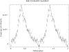 |
Fig. A.1. IGR J19140+0951 orbital profile obtained from the Swift/BAT light curve (15–50 keV energy range) folded at the newly refined period of 13.55273 d over 64 bins. The assumed reference time is MJD 52061.42 and the data span from 2005-0-15 to 2022-01-18. The profile is displayed twice for clarity. |
Appendix B: IGR J17315−3221
IGR J17315−3221 was reported for the first time in the catalog of the INTEGRAL sources published by Krivonos et al. (2012) and suspected to be another HMXB discovered by INTEGRAL, possibly a SgXB (see also Clavel et al. 2019). The source is reported in the catalog at a best determined position of RA = 262.818, DEC=-32.306, with an associated positional accuracy of 2 arcmin. The estimated average flux in the 17-60 keV energy band was 4×10⁻¹² erg cm2 s−1. We show here that the reported discovery of this source is most likely the result of an artifact of the INTEGRAL data analysis; a re-analysis of all available INTEGRAL data show no evidence of a significant source detection at a position consistent with that reported previously for IGR J17315−3221.
As IGR J17315−3221 was initially announced to be a likely additional HMXB discovered by INTEGRAL, this source was included among the monitored targets in our observational campaigns carried out with Swift. XRT performed observations in the direction of the source between 2012 and 2016, for a total available exposure time of 12.1 ks (see Table B.1, where the target ID 34659 identifies our ten 1 ks pointed observations, the remainder being archival ones). We first extracted an image of the XRT field of view for each observation and then a single image stacking all data together in the 0.3–10 keV energy band. No X-ray source is detected within 2 arcmin from the best reported position of IGR J17315−3221 in the single images or in the stacked image obtained with all available data. A 3 σ upper limit in the 0.3–10 keV was calculated by using SOSTA within the XIMAGE task and a circular background region (radius of 56 pixels) away from field sources, at 1.7 × 10⁻³ cts s−1; by using PIMMS (v4.11b), when assuming a photon index of 2.1 and an absorbing column of 1.23 × 1022 cm−2, we obtain an observed (unabsorbed) flux of 9.9 × 10⁻¹⁴ (2.30 × 10⁻¹³ erg cm2 s−1).
Swift/XRT observation log for IGR J17315+3221.
Motivated by the lack of any soft X-ray counterpart in the XRT data, we reanalyzed all the INTEGRAL archival data available around the position of IGR J17315−3221. Using the latest available calibration and software version (Offline Scientific Analysis 11.2) from the multi-messenger online analysis platform6, we extracted a mosaic image in the 20–60 keV energy band using first the same IBIS/ISGRI data considered by Krivonos et al. (2012) and then from 2014 to 2021 (restricting the pointings to a maximum allowed off-axis angle of 12° to avoid large instrument systematics7). Neither of the two images shows a significant detection of any source at a location compatible with the reported position of IGR J17315−3221. From January 2004 to December 2012, we obtained a 3 σ upper limit on the source flux in the 20–60 keV energy band of 0.4 mCrab (5 × 10⁻¹² erg s−1 cm−2) in 4.2 Ms of effective exposure on the source. From January 2013 to October 2021, we obtained a slightly worse upper limit of 0.6 mCrab (7 × 10⁻¹² erg s−1 cm−2) in 3.7 Ms, owing to the degraded instrument response at low energy during the mission lifetime. To obtain these upper limits, we elaborated the original mosaics using Sextractor (Bertin & Arnouts 1996) in its most recent implementation (version 2.25.2)8. This was done to correct for the coding noise that is particularly pronounced in the Galactic center region, due to the large number of bright sources and diffuse emission. We applied the software with a box size of four pixels and a detection threshold for sources of three. We show the cleaned significance map for the period 2004–2012 in Fig. B.1; the map in the following period is similar.
 |
Fig. B.1. INTEGRAL IBIS/ISGRI significance map in the 20–60 keV energy range of the region around IGR J17315−3221 obtained from all available pointings at less than 12 degrees from the source collected in the time period 2004–2012. No significant detection of the previously reported source could be found. |
From this re-analysis of INTEGRAL data and the Swift/XRT non-detection, we conclude that IGR J17315−3221 is not a real astrophysical source, but rather an analysis artifact.
Appendix C: Swift data log tables
In the following tables we show the logs of the Swift observations that we analyzed for each source included in the paper. In Tables C.1–C.3, the columns represent the observing sequence, observation date (mid-observation MJD), orbital phase, start and end times of the observations (UT), exposure time in seconds, and the 0.3–10 keV flux in units of 10−11 erg cm−2 s−1. The missing values are due to insufficient counts, which prevented any spectral analysis. In the case of XTE J1855−026 (Table C.4), also the log of the BAT data are reported. We note that in these tables the uncertainties are at 90% confidence level. In Tab. C.5, we show the Swift/XRT observation log for IGR J17503−2636 together with the spectral fit results.
Swift/XRT observation log for 4U J1907+097.
Swift/XRT observation log for IGR J19140+0951.
Swift/XRT observation log for IGR J16393−4643.
Swift observation log of XTE J1855−026
Swift/XRT observation log and spectral fit results for IGR J17503−2636.
All Tables
Best-fit parameters obtained from the XMM-Newton data of 4U 1907+09 collected during the observation 0555410101.
Results of the orbital-phase-resolved spectral analysis conducted on the Swift/XRT observations of IGR J19140+0951.
Best-fit parameters of the XMM-Newton observation of IGR J18410−0535 carried out in 2020 (OBSID 0862410101).
Results of the orbital-phase-resolved spectral analysis conducted on the Swift/XRT data of IGR J16393−4643.
All Figures
|
Fig. 1. Swift/XRT hardness ratio of 4U 1907+09, and best-fit parameters as a function of orbital phase (absorption column density NH in units of 1022 cm−2, power-law photon index Γ, and 0.3–10 keV flux not corrected for absorption in units of 10−10 erg cm−2 s−1). |
| In the text | |
|
Fig. 2. 4U 1907+09 unfolded spectra obtained by using the entire exposure time available in the XMM-Newton OBSID 0555410101 for the EPIC-pn (black points), MOS1 (red crosses), and MOS2 (blue circles) cameras. The residuals from the best-fit model are reported in the bottom panel. |
| In the text | |
|
Fig. 3. Timing analysis of 4U 1907+09. Top left, panel a: hardness ratio of the combined EPIC-pn, MOS1, MOS2 light curves (3–10 keV/0.5–3 keV). Top left, panel b: total rate in the 0.5–10 keV energy range. Bottom left, panel c: distance dj from the average for each pulse profile as function of HR. Bottom left, panel d: distance dj from the average for each pulse profile as function of the total rate. The numbers indicate the different intervals identified in panel b (see Eq. (1) for the definition of dj). Right: plot of the best-fit parameters as a function of time obtained from the HR-resolved spectral analysis of the XMM-Newton observation of 4U 1907+09. The parameters reported in the different panels are those introduced in Table 2 and described in the text. |
| In the text | |
|
Fig. 4. Average and HR-resolved pulse profiles of 4U 1907+09 divided by their mean and vertically displaced by ten times their distance from the average, as computed in Eq. (1). The symbols represent the pulse profile as labeled in panel a of Fig. 3. |
| In the text | |
|
Fig. 5. Same as Fig. 1, but for IGR J19140+0951. Here the flux is given in units of 10−11 erg cm−2 s−1. |
| In the text | |
|
Fig. 6. Plot of light curve, HR, and best-fit parameters as a function of time obtained from the HR-resolved spectral analysis of the XMM-Newton observation of IGR J11215−5952. Panel a: source count rate in the 0.5–10 keV bands, after adaptive rebinning with minimum S/N of 15 in the light curve extracted for 0.5–3 keV; panel b: HR between the 3–10 keV and 0.5–3 keV energy-resolved light curves with the identified time intervals for the spectral extraction (red lines); panel c: f, covering fraction of the partial absorber; panel d: Γ, power-law photon index; panel e: NH, absorption column density along the direction to the source (including Galactic absorption); panel f: NH, pc, absorption column density of the partial absorber (representing the absorption column density local to the source; PCFABS in XSPEC); panel g: F2 − 10 keV, measured power-law flux in the 2–10 keV energy range not corrected for absorption for the EPIC-pn in units of 10−12 erg s−1 cm−2. |
| In the text | |
|
Fig. 7. Timing analysis of the of the 2020 observation of IGR J18410−0535 (OBSID 0862410101). Lower panel: combined EPIC-pn+MOS1+MOS2 light curve in 0.5–10 keV energy range. Upper panel: hardness ratio between the light curves in the bands 3.5–10 keV and 0.5–3.5 keV rebinned at a minimum S/N of 8. There are no significant variations in the hardness ratio, and thus the Bayesian algorithm identified a single time interval for the spectral extraction (red lines, corresponding to the whole observation). |
| In the text | |
|
Fig. 8. Same as Fig. 1, but for IGR J16393−4643. Here the flux is given in units of 10−11 erg cm−2 s−1. |
| In the text | |
|
Fig. 9. Light curves of the 2011 September 18 outburst of XTE J1855−026 caught by BAT and XRT. Panels a–d: BAT light curves (c s−1, at 10 s binning); panel e: XRT light curve (0.3–10 keV c s−1); the horizontal red line indicates the time where the BAT event data were collected. A different scale is used for the x-axis. |
| In the text | |
|
Fig. 10. Timing analysis of the XTE J1855−026outburst. Panel a: XRT hard-band light curve (4–10 keV c s−1); panel b: soft-band light curve (0.3–4 keV c s−1); panel c: hardness ratio (4–10 keV/0.3–4 keV). WT data are shown in blue, PC data in red. |
| In the text | |
|
Fig. 11. Spectroscopy of the 2011 September 18 outburst of XTE J1855−026. Top panel: unfolded spectra of the nearly simultaneous XRT/WT1 data (blue crosses) and BAT DPH1 data (empty black circles) fit with an absorbed cut-off power-law model. Bottom panel: data/model ratio of the fit. |
| In the text | |
|
Fig. 12. Spectroscopy of the 2011 September 18 outburst of XTE J1855−026. Top panel: unfolded spectra of the simultaneous XRT/PC1 data (red crosses), the BAT DPH2 data in black (filled circles), and the BAT DPH3 data in gray (empty circles) fit with an absorbed cut-off power-law model. Bottom panel: data/model ratio of the fit. |
| In the text | |
|
Fig. 13. Long-term light curve of IGR J17503−2636 as measured by Swift /XRT. For completeness, we included the XRT observations already published in our previous paper on the source (MJD 58343 and 58333, Ferrigno et al. 2019). |
| In the text | |
|
Fig. A.1. IGR J19140+0951 orbital profile obtained from the Swift/BAT light curve (15–50 keV energy range) folded at the newly refined period of 13.55273 d over 64 bins. The assumed reference time is MJD 52061.42 and the data span from 2005-0-15 to 2022-01-18. The profile is displayed twice for clarity. |
| In the text | |
|
Fig. B.1. INTEGRAL IBIS/ISGRI significance map in the 20–60 keV energy range of the region around IGR J17315−3221 obtained from all available pointings at less than 12 degrees from the source collected in the time period 2004–2012. No significant detection of the previously reported source could be found. |
| In the text | |
Current usage metrics show cumulative count of Article Views (full-text article views including HTML views, PDF and ePub downloads, according to the available data) and Abstracts Views on Vision4Press platform.
Data correspond to usage on the plateform after 2015. The current usage metrics is available 48-96 hours after online publication and is updated daily on week days.
Initial download of the metrics may take a while.