| Issue |
A&A
Volume 664, August 2022
|
|
|---|---|---|
| Article Number | A49 | |
| Number of page(s) | 13 | |
| Section | Galactic structure, stellar clusters and populations | |
| DOI | https://doi.org/10.1051/0004-6361/202141895 | |
| Published online | 04 August 2022 | |
Radio observations of massive stars in the Galactic centre: The Quintuplet cluster
1
Instituto de Astrofísica de Andalucía (IAA-CSIC), Glorieta de la Astronomía s/n, 18008 Granada, Spain
e-mail: This email address is being protected from spambots. You need JavaScript enabled to view it.
2
Centro de Astrobiología (CSIC/INTA), Ctra. de Ajalvir Km. 4, 28850 Torrejón de Ardoz, Madrid, Spain
3
CIERA, Department of Physics and Astronomy Northwestern University, Evanston, IL 60208, USA
4
Max-Planck-Institut für Astronomie, Königstuhl 17, Heidelberg 69 117, Germany
Received:
28
July
2021
Accepted:
13
December
2021
Abstract
We present high-angular-resolution radio continuum observations of the Quintuplet cluster, one of the most emblematic massive clusters in the Galactic centre. Data were acquired in two epochs and at 6 and 10 GHz with the Karl G. Jansky Very Large Array. With this work we have quadrupled the number of known radio stars in the cluster. Even though the uncertainty of the measured spectral indices is relatively high, we tentatively classify the 30 detected stars. Eleven have spectral indices consistent with thermal emission from ionised stellar winds, ten have flat to inverted spectral indices indicative of non-thermal emission arising in colliding winds in binaries, and the nine remaining sources cannot be easily classified because of large uncertainties or extremely positive values of the spectral index. The mean mass-loss rate estimated for Wolf-Rayet stars agrees with previous work. Regarding variability, remarkably we find a significantly higher fraction of variable stars in the Quintuplet cluster (∼30%) than in the Arches cluster (< 15%), probably because the Quintuplet cluster is older. Our determined stellar wind mass-loss rates are in good agreement with theoretical models. Finally, we show that the radio luminosity function can be used as a tool to constrain the age and the mass function of a cluster.
Key words: open clusters and associations: individual: Quintuplet / radio continuum: stars / stars: massive / stars: mass-loss / stars: luminosity function, mass function
© ESO 2022
1. Introduction
The Quintuplet cluster, along with the Arches and the Central Parsec clusters, is a young massive stellar cluster in the Galactic centre (GC). Separated just a few arcminutes from the Arches cluster, the Quintuplet cluster is located at a projected distance of approximately 30 pc (or 12.5 ′ in angular distance) to the north-east of Sagittarius A* (Sgr A*), the black hole at the centre of our Galaxy. Given its position at the GC, Quintuplet can only be observed (in addition to radio frequencies) at infrared wavelengths, which poses a difficulty in identifying its stellar content because intrinsic stellar colours are small in the infrared, and reddening and the related uncertainty will dominate the observed colours (Nogueras-Lara et al. 2018, 2021).
The Quintuplet cluster owes its name to five prominent infrared-bright sources, later named Q1, Q2, Q3, Q4, and Q9 by Figer et al. (1999; see Fig. 1). Its mass is similar to that of the Arches cluster, about 1−2 × 10⁴ M⊙ (Figer et al. 1999; Rui et al. 2019); however, it is considered to be roughly 1 Myr older (Arches: 2.5−4 Myr, Quintuplet: 3−5 Myr; Figer et al. 1999; Clark et al. 2018a,b; Schneider et al. 2014). This is reflected in its larger core radius, probably a sign of its ongoing dissolution in the GC tidal field (Rui et al. 2019), and its content of more evolved stars than the Arches cluster (Clark et al. 2018b). The extended nature of Quintuplet poses a problem with respect to confusion with the mostly old stars of the nuclear stellar disc in which it is embedded (Nogueras-Lara et al. 2019a; Launhardt et al. 2002). In addition, interlopers of young stars that have formed in the vicinity of the Quintuplet cluster, but at a somewhat different time, may also be present (Clark et al. 2018b).
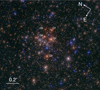 |
Fig. 1. JHK false colour image of the Quintuplet cluster from the GALACTICNUCLEUS survey. Credits: Nogueras-Lara et al. (2018,2019b). |
Massive young stellar clusters are of great interest to study the evolution of the most massive stars, those with masses in excess of a few tens of solar masses. The observable number of such stars in the Milky Way is small; they are very rare due to the stellar initial mass function that is a steep power law of mass (Hosek et al. 2019) and due to the very short lifetimes of these stars (at most a few Myr). The latter means that massive stars are typically located at distances of many kiloparsecs from Earth, and also that they are frequently still enshrouded in dusty molecular clouds and are therefore highly extinguished. Because they are two of the most massive young clusters in the Milky Way, the Arches and the Quintuplet have been the objects of intense study over the past three decades (Figer et al. 1999; Najarro et al. 2009, 2017; Clark et al. 2018b; Liermann et al. 2009, 2010, 2012; Hosek et al. 2019, among others), driven by ever-improving infrared imaging and spectroscopy instruments. Imaging, spectroscopic, and proper motion measurements in the infrared have provided us with our current ideas of mass, age, and metallicity of these clusters as the spectral types and mass of their ∼100 most massive stars, as described in the references cited above.
Highly complementary information on the properties of massive young stars can be obtained from radio observations. Radio continuum emission arises in the ionised winds of massive stars (see e.g. Bieging et al. 1989; Leitherer et al. 1997; Scuderi et al. 1998; Güdel 2002; Umana et al. 2015) and can provide essential information on mass-loss rates through stellar winds. Lang et al. (2005) carried out a multi-frequency, multi-configuration, and multi-epoch study of the Arches and Quintuplet clusters with the Very Large Array (VLA). They detected ten relatively compact radio sources. The majority of them had rising spectral indices, assuming the relation Sν ∝ να, with ν the observing frequency and Sν the measured flux density, as expected for young massive stars with powerful stellar winds. A few sources had clear near-infrared (NIR) counterparts.
In this work we study Quintuplet with the Karl G. Jansky Very Large Array (JVLA), taking advantage of the significantly increased sensitivity in comparison with the old VLA, as we did for the Arches cluster aiming to pick up the thermal and non-thermal emission from the ionised gas in the outer wind regions of young massive stars (see Gallego-Calvente et al. 2021).
2. Observations and imaging
We observed the radio continuum emission from the Quintuplet cluster using the National Radio Astronomy Observatory (NRAO)1 JVLA in 2016 and 2018. We acquired data in two bands (C and X), with X-band observations in three epochs, as detailed in Table 1.
Summary of observations.
The phase centre was taken at the position α, δ(J2000) = 17h46m15.26s, −28°49′33.0″. All observations were carried out in the A configuration to achieve the highest angular resolution. This configuration also helped us to filter out part of the extended emission that surrounds the Quintuplet cluster whose centre is located at a few arcminutes to the south-east of the Sickle H II region (G0.18−0.04) and at approximately 10″due north of the Pistol (G0.15−0.05) H II region. J1744−3116 was used as phase calibrator and J1331+305 (3C286) as band-pass and flux density calibrator at all frequencies.
The raw data were processed automatically performing an initial flagging and calibration through the JVLA calibration pipeline. Extra flagging was necessary to remove lost or corrupted data. The entire cluster was visible within the field of view (FoV) of the observations. The FoV can be defined as the FWHM of the primary beam of the VLA antennas (PB):  arcmin (8.4′ and 4.2′ in the C and X bands, respectively).
Properties of the images.
A very bright source was present in the FoV in both bands. This source is located at α, δ(J2000) = 17h46m21.04s, −28°50′03.11″. We identified it as SgrA-N3 using the VizieR Catalogue Service2. We carried out data reduction with the Common Astronomy Software Applications package (CASA) developed by an international consortium of scientists3 as follows.
We used the task tclean to create a model for the intense source in order to, later on, self-calibrate on this source. To filter out some of the extended emission near and around the target field we constrained the u − v range by excluding baselines shorter than 6000 m (10 000 m) at 10 GHz (6 GHz), because our goal was to detect the compact sources. These values turned out to be optimal after performing several tests. These two steps (i.e. model generation and calibration of the time-dependent antenna-based gains on the bright source) were repeated several times, thereby iteratively changing the parameter that controls the solution interval, solint, in the gaincal task. An improvement of 15% in the dynamic range was achieved through this iterative approach. We inserted the final model by means of the task ft from CASA. Since the diffraction pattern residuals of the bright (∼40 mJy) SgrA-N3 source interfered with our aim to detect faint sources, we subtracted it in the Fourier plane. Subsequently, we cleaned our new visibility data set, stored in a new table as a Measurement Set (MS), using tclean in interactive mode. We chose the interactive mode because the subtraction of SgrA-N3 was not completely perfect and the restriction of the u − v range did not entirely remove the extended emission.
We attempted to improve the images in all epochs through testing the more advanced form of imagingmulti-scale clean, which distinguishes emitting features with angular scales between point sources and extended emission. Its use did not improve the quality of the final images. Additionally, we probed different weighting schemes to correct for visibility sampling effects. The natural weighting scheme resulted in the images with the highest signal-to-noise ratio (S/N). The gain parameter in the clean algorithm was set to 0.05. With this procedure we reached an off-source rms noise level of 4.3 μJy beam−1 in the 2016 X-band image in the central regions of the FoV. The off-source thermal noise in the 2018 epochs was 5.7 and 6.6 μJy beam−1 for X and C bands, respectively.
All the images were primary-beam corrected to account for the change in sensitivity across the primary beam. Table 2 summarises the properties of the final images.
3. Results
3.1. Point source detection and flux density
Point sources were selected interactively in the cleaning procedure, as we specified in Sect. 2; we restricted ourselves to those at above five times the off-source rms noise level. We used the image-plane component fitting (imfit) task from CASA that takes into account the quality of the fit and each image rms to estimate the positions of the maxima, the total flux densities, and the errors of these values over the final primary-beam-corrected images for all bands in all epochs. We determined the uncertainties in the positions of the detected sources by adding in quadrature to the formal error of the fit, 0.5 θ/SNR (Reid et al. 1988), a systematic error of 0.05″ (Dzib et al. 2017). In the formal error, θ is the source size convolved with the beam and SNR the S/N. The systematic error addresses the thermal noise and uncertainties introduced by the phase calibration process. Likewise, we considered the percentage in the calibration error of the peak flux densities at the observed frequencies (Perley & Butler 2013) and the factor that considers whether a source is resolved or unresolved to evaluate the flux-density uncertainties.
This process led us to detect 29 and 28 point sources above 5σ at 10 GHz and 6 GHz, respectively. Figure 2 shows a closeup of the 2016 X-band image and a closeup of the 2018 C-band image of the cluster, both images corrected for primary-beam attenuation, with radio stars labelled. We note that some of the detected point sources lie outside of the FoV shown in the figure.
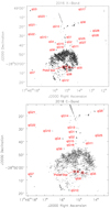 |
Fig. 2. Detected point sources above 5σ at 10 GHz and 6 GHz. Top: closeup of the Quintuplet cluster from the 2016 X-band image corrected for primary-beam attenuation. The clean beam is 0.47″ × 0.15″, PA = 25.29°. The off-source rms noise level is 4.3 μJy beam−1. The contour levels represent −1, 1, 2, 3, 4, 5, and 6 times 5 σ. Bottom: closeup of the Quintuplet cluster showing most of the detected sources from the 2018 C-band image corrected for primary-beam attenuation. The resolution is 0.62″ × 0.21″, PA = 19.97°. The off-source rms noise level is 6.6 μJy beam−1. The contour levels represent −1, 1, 2, 3, 4, 5, and 6 times 5 σ. |
The 2016 X-band image turned out to be the image with the highest S/N, so it provides the most complete list of point sources. Besides the rms noise, there is systematic noise present in the radio image, caused by remnant side lobes of SgrA-N3 that could not be fully removed from the image, and some diffuse flux still present in the u − v range considered for the image reconstruction. In addition, the Quintuplet region is full of ionised gas in clouds of variable compactness. The systematic noise and the ionised gas can give rise to numerous spurious detections, even at 5σ above the rms noise. Therefore, we compared the positions of detected radio point sources in our 2016 X-band image with the positions of stars on an HST/WFC3 F153M image of the Quintuplet cluster (Rui et al. 2019), downloaded from the HST archive4. All radio stars must necessarily be very bright infrared sources (massive young stars) that are detected at S/N values exceeding a few times 100. Only sources coincident within 0.05″ of the position of stars detected in the NIR were accepted as real. The tagged HST/WFC3 F153M image is shown in Fig. 3.
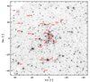 |
Fig. 3. HST/WFC3 F153M image of the Quintuplet cluster with identified radio stars labelled. |
Finally, we matched our sources with the ones provided by Tables A.1 and A.2 in Clark et al. (2018b), based on HST/NICMOS+WFC3 photometry and VLT/SINFONI+ KMOS spectroscopy for ∼100 and 71 cluster members, respectively. In this way we were able to obtain the spectral type of the radio stars.
Lang et al. (2005) reported nine compact radio sources and the Pistol Star. They referred to the former as QR1−QR9. QR1−3 were interpreted as the first detections of embedded massive stars in the Quintuplet cluster. As we can see in Fig. 3, these sources have no bright stellar NIR counterparts, as was clearly indicated by Lang et al. (2005) as well. To further investigate these sources, we superposed the HST/WFC3 F153M image from HST archive with a Paschen α image by Dong et al. (2011), see Fig. 4. From this figure we can see that QR1−3 are not stellar sources but are related to ionised gas clouds that have a similar appearance to many other such objects in this region.
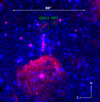 |
Fig. 4. Composition of the HST/WFC3 F153M image from HST archive with a Paschen α image by Dong et al. (2011). Blue: HST WFC3 F153M; Red: HST NIC3 Paschen α. The QR1−3 sources by Lang et al. (2005) are encircled. |
Considering this finding, we have renamed the Quintuplet cluster members to reassign a number to the detected radio sources from #1 to #29. We do not use the prefix QR used by Lang et al. (2005) to avoid confusion between the old QR1−3 and the new 1−3 numbered members, so we introduce a new prefix, qG. We confirm seven sources reported by Lang et al. (2005) as radio stars (QR4, QR5, QR6, QR7, QR8, QR9, Pistol Star). With a total of 29 sources reported here, this work quadruples the number of known radio stars associated with the Quintuplet cluster, with the faintest radio source having a flux density of 30 ± 7 μJy at X band.
Table A.1 shows the new and the old nomenclature, the identified NIR counterparts as listed in Clark et al. (2018b), determined positions, the X- and C-band flux densities for all radio sources measured in our 2016 and 2018 data sets or the upper limits of the undetected sources, and the spectral classification according to Clark et al. (2018b).
3.2. Spectral indices
We calculated the spectral indices (or their limits) of the radio stars, as well as the corresponding uncertainties using their measured X- and C-band fluxes. We proceeded as described in Gallego-Calvente et al. (2021). The spectral indices are listed in Col. (8) of Table A.1.
3.3. Mass-loss rates
We determined the mass-loss rates for the detected radio stars following the recipe described in Gallego-Calvente et al. (2021). We derived mass-loss rates corresponding to the observed flux densities at 6 GHz (C band) and 10 GHz (X band), assuming that the observed radio emission is due to free-free emission from ionised extended envelopes with a steady and completely ionised wind, with a volume filling factor f = 1, and an electron density profile ne ∝ r−2. For values of f < 1 our mass-loss rates must be multiplied by  , such that the mass-loss rate for f = 1 would be the maximum one. In the case of non-thermal contributions, our values (shown in Table A.2) represent upper limits to the true mass-loss rates.
For most Quintuplet cluster members, we can assume that helium stays singly ionised in the radio emitting region of the stellar wind, so the number of free electrons per ion and the mean ionic charge can be set γ = 1 = Z (Leitherer et al. 1997). However, in the case of the two luminous blue variables (LBVs), the Pistol Star and qG3, accounting for the fact that helium is predominantly neutral in the winds of these cool stars, we take γ = 0.8 and Z = 0.9, similarly to other LBV studies (e.g. Leitherer et al. 1995; Agliozzo 2019).
Table A.2 also shows the estimations done by Lang et al. (2005) from their 22.5 GHz flux densities when possible, and otherwise from their 8.5 GHz flux densities. They used their higher frequency observations as better tracers of the thermal component, and so give more reliable mass-loss rates because contamination of the flux density by the non-thermal component can occur at the lower frequencies (according to Contreras et al. 1996, among others). Lang et al. (2005) assumed a terminal wind velocity of 1000 km s−1 and a mean molecular weight equal to 2 for all sources. Thus, in order to compare our data with their data, we rescaled Lang’s values multiplying them by v∞/1000 and μ/2, where v∞ and μ are the values adopted in this work. We derived a significantly lower mass-loss rate for the Pistol Star than Lang et al. (2005); the latter work reports a roughly ten times higher flux density for this source. This may be explained through variability of the source (see below) or, possibly, the lower angular resolution of the observations of Lang et al. (2005), which may have resulted in the flux of the Pistol Star being contaminated by flux coming from the Pistol nebula, where it is embedded. Similar discrepancies exist for the sources qG13/QR4 and qG11/QR7.
We note that the estimated mass-loss rates show some differences between the C and the X bands by up to a few tens of percent. On average, mass-loss rates inferred in the C band are about 80% of those in the X band. This may be due to various reasons. For example, the mass-loss rates are estimated based on an idealised model of thermal winds. Thermal emission rises towards higher frequencies, while contamination from non-thermal effects can be significant in the C band. The lower angular resolution in the C band in this highly complex field may also bias the C-band estimates. In conclusion, the X-band mass-loss rates can be considered more reliable.
4. Properties of the sources
According to the spectral classification, most of the detected sources in the Quintuplet cluster are young massive post-main sequence stars, being the majority of the Wolf-Rayet spectral type (see Table A.1). In particular, two luminous blue variables, eight WC, six WN, seven B supergiants, and three sources of type O Ia have been found.
Leitherer et al. (1997) suggested that there is little variation in the mass-loss rates for Wolf-Rayet stars, with an average value of ∼4 × 10⁻⁵ M⊙ yr−1. Similar mean mass-loss rates for WR stars were found in more recent work (Cappa et al. 2004; Montes et al. 2015). The WR stars from our data set have Ṁ values ranging from 1.3 × 10⁻⁵ to 7.9 × 10⁻⁵ M⊙ yr−1. The mean WR mass-loss rate of our sample at 10 GHz is 4 ± 2 × 10⁻⁵ M⊙ yr−1, which agrees well with the previous measurements. This conclusion lead us to choose B1−2 Ia+ and B0−1 Ia+ as the most probable spectral types for qG13 and qG17, respectively, as their mass-loss rates are not in that range.
The spectral index, α, provides us with information about the nature of the observed emission. A value of α ≈ 0.6 is consistent with thermal emission, while a flat or negative α is indicative of non-thermal emission. The uncertainties of the spectral indices measured here are large, but we tentatively group the stars into three classes: (1) thermal emitters with α ≈ 0.6; (2) non-thermal emitters with a zero or negative α, considering the 1σ uncertainties in both cases; and (3) ambiguous sources, with very large uncertainties or values of α > 1.
With these criteria, qG2, qG4, qG6, qG10, qG13, qG14, qG15, qG17, qG18, qG23, and qG24 have spectral indices consistent with thermal emission from ionised stellar winds. On the other hand, qG1, qG5, qG7, qG8, qG9, qG11, qG16, qG19, qG20, and qG29 have flat or inverted spectral indices, which indicates the presence of non-thermal emission that may be attributed to colliding winds in binaries. Ambiguous cases are the Pistol Star, qG3, qG12, qG21, qG22, qG25, qG26, qG27, and qG28.
In thermal emitters, the divergence of α from the canonical value of 0.6 can occur for a number of reasons, such as deviations in the wind conditions possibly due to the presence of condensations (clumps) that produce a non-standard electron density profile (ne ∝ r−s, with s ≠ 2) and/or non-standard ionisation profiles or wind geometry (e.g. due to internal shocks). Flat to inverted spectra (α ≲ 0) can be found in binaries as a result of the contribution of non-thermal emission in colliding wind regions, provided this emission is not absorbed by the surrounding ionised wind, which is optically thick (Benaglia 2010; Montes et al. 2015). Thus, identifying binaries through radio observations is typically limited to the detection of wide binaries with periods of one year or longer (Sanchez-Bermudez et al. 2019). Therefore, in these systems, only the free-free thermal emission from the unshocked winds is thought to be detected, thereby masking any effect of their binarity. We can therefore not exclude that the systems with thermal emission are also binaries. Since most massive stars are born in multiples (e.g. Mason et al. 2009; Sana et al. 2011; Sota et al. 2014), this is rather likely.
In some short-period systems (depending on the geometry of the binary and of its interacting winds), emission from the shock region may escape, contributing to a composite spectrum with a flat spectral index at certain orbital phases in systems with significant eccentricity. This non-thermal emission can appear to be modulated by the orbital motion of the system (only if the orbit is non-circular), resulting in variability of the total spectrum with a periodicity related with the orbital period.
We can probe the existence of long-term variability since we have two epochs with X-band measurements. We contemplate the existence of flux density variability when the differences in the flux densities between the two epochs are higher than 5σ. With this criterion we consider the two LBVs (qG3 and the Pistol Star) as variable sources, as well as the sources qG1, qG8, qG12, qG20, and qG29. For qG10 and qG11 the variability is rather small, but taking into account the possible binary nature of qG11, we speculate that the contribution from non-thermal emission may be modulated by the orbital motion of the system, although there are other factors that may modulate the radio emission, such as projection effects, inclination, or dust creation. Further investigation would be necessary to find a correlation between the periodicity and the orbital period. In conclusion, we find that 9 out of the 29 radio sources, approximately 30%, display significant variability. This is a remarkably higher fraction than in the Arches cluster, where we find that ≲15% of the radio stars display variability (see Gallego-Calvente et al. 2021). We speculate that this may be related to the advanced evolutionary state of the older Quintuplet stars.
5. Analysis of the radio luminosity function
5.1. Basic assumptions
With assumptions about the age and mass of a young cluster, a comparison between the number and the observed flux of detected radio stars with predictions from theoretical stellar evolutionary models (isochrones) can help to assess the quality of these models, and also, if the theoretical isochrones are considered sufficiently reliable, to infer basic properties of the cluster. In Gallego-Calvente et al. (2021) we show that the observed number of radio stars in the Arches cluster appears to require a top-heavy initial mass function with a power-law exponent αIMF = −1.8 (at odds with the solar environment Salpeter exponent αIMF = −2.35).
In this work we tentatively take a step further and use the radio luminosity function (RLF) of the stars: we use the number of sources as well as their flux density for comparison with the models. We do this first for the Arches cluster and then for the Quintuplet cluster. We note that we cannot undertake an exhaustive study here, which would require taking into account a large number of potentially important parameters, such as the role of metallicity or the wind volume filling factor, which we neglect here. Nevertheless, with these basic assumptions we show that our simple toy modelling indicates that current theoretical models of the evolution of massive stars appear to be fairly realistic, and that we can infer constraints on the properties of the clusters by comparing radio observations with predictions from isochrones.
We use PARSEC5 (release v1.2S + COLIBRI S_37; Bressan et al. 2012; Chen et al. 2014, 2015; Tang et al. 2014; Marigo et al. 2017; Pastorelli et al. 2019, 2020) and MIST6 (Dotter 2016; Choi et al. 2016; Paxton et al. 2011, 2013, 2015) theoretical isochrones for solar metallicity. To convert the mass-loss rates from the theoretical isochrones to observable radio flux, we use the relation
![Mathematical equation: $$ \begin{aligned} \biggl [ \frac{S_{\nu }}{{\mathrm{mJy}}} \biggr ]&= (5.34 \times 10^{-4})^{-4/3}\, f^{1/2}\,\biggl [\frac{\dot{M}}{{M}_{\odot }\,\mathrm{yr}^{-1}} \biggr ] \biggl [ \frac{{v}_{\infty }}{\mathrm{km\,s}^{-1}}\biggr ]^{-4/3} \nonumber \\&\qquad \biggl [ \frac{d}{\mathrm{kpc}}\biggr ]^{-2}\, \biggl [ \frac{\nu }{\mathrm{Hz}}\biggr ]^{2/3}\,\biggl [ \frac{{\mu }^{2}}{Z^{2} \gamma g_{\nu }}\biggr ]^{-2/3}, \end{aligned} $$](/articles/aa/full_html/2022/08/aa41895-21/aa41895-21-eq3.gif) (1)
(1)
which has been reported before in similar versions (e.g. Gallego-Calvente et al. 2021; Montes et al. 2009; Leitherer et al. 1997). The observing frequency is ν = 10 GHz. We assume typical values, with a mean molecular weight μ = 1.3, a mean ion charge Z = 1, and a mean number of electrons per ion γ = 1. For the Gaunt factor,
 (2)
(2)
we use Te = 104 K. Any changes to these assumed values of the parameters by factors of two to a few do not significantly change the resulting radio flux. A potentially important factor that we have not yet mentioned is wind clumping. The volume filling factor, f, is one for a homogeneous stellar wind and smaller than one for a clumpy wind. For simplicity, we here assume f = 1.
The validity of such a rule-of-thumb approach is demonstrated in Fig. 5, where we compare the observed flux densities of radio stars in the Arches cluster with those computed from their individually determined mass-loss rates (Gallego-Calvente et al. 2021) and using the simplified assumptions. The differences appear to be small enough to justify an efficient simplified computation of the radio flux densities. From here on we use these simplified assumptions on the parameters that enter Eq. (1), and only consider the observed radio flux densities, not the mass-loss rates.
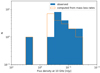 |
Fig. 5. Histogram of Sν of observed radio stars in Arches cluster. Blue solid histogram: Observed flux densities of radio stars in the Arches cluster (Gallego-Calvente et al. 2021). Orange outline: Radio fluxes of the same stars, using the mass-loss rates reported by Gallego-Calvente et al. (2021) and converting to radio flux density with Eq. (1) assuming the same parameters for all stars. |
For our cluster models we always use a one-segment power-law initial mass function (IMF) with an upper mass of 150 M⊙ and a lower mass of 0.8 M⊙. Our results are not sensitive to reasonable changes in these parameters. In addition, since our sources of interest represent only the very tip of the mass distribution, assuming a two-segment IMF does not introduce any significant changes.
We tested whether the random sampling of the high-mass end of the IMF is biasing our results by random realisations of clusters of given age, mass, and IMF. We only used MIST models for this test and assumed that we could only detect stars with a radio flux density ≳0.04 mJy, the approximate detection limit here and in Gallego-Calvente et al. (2021). We found that the age of the clusters can typically be recovered well (±1 Myr) and that the cluster parameters could best be recovered for an age of ∼3 Myr, where the number of bright radio stars peaks. Whether the IMF was top-heavy or not could also be recovered with great reliability. However, we found a degeneracy between the RLFs for the ages of 2 and 6 Myr. Since these values lie safely outside (or at the very extreme of) the ages reported for the Arches and Quintuplet clusters, we do not use them in our subsequent analyses.
5.2. Models
Figure 6 shows predictions at two different ages for a model cluster with a total initial stellar mass of 104 M⊙ and a power-law IMF with an exponent αIMF = −1.8 (Hosek et al. 2019), using MIST isochrones. We averaged and used the 1σ confidence intervals of the result of ten simulations of the cluster. The upper panel shows the present-day mass function, the middle panel shows histograms of the predicted radio flux density, and the lower panel shows cumulative histograms of the predicted radio flux density. Observed values in Arches and Quintuplet are overplotted in black. Finally, we show the same models, created with PARSEC isochrones, in Fig. 7. We can see differences due to the use of different theoretical isochrones, but we can also see the overall similarity of the predictions.
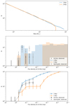 |
Fig. 6. Radio flux densities of massive stars in a model cluster, using MIST isochrones. Top: present-day mas function. Middle: histograms of predicted radio flux densities. Bottom: cumulative histograms of predicted radio flux densities. The black histogram corresponds to the observed data for the Arches cluster (Gallego-Calvente et al. 2021, dotted) and the grey histogram to the observed data for the Quintuplet cluster (this work, solid). |
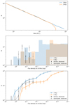 |
Fig. 7. Radio flux densities of massive stars in a model cluster, using PARSEC isochrones. Top: present-day mas function. Middle: histograms of predicted radio flux densities. Bottom: cumulative histograms of predicted radio flux densities. The black histogram corresponds to the observed data for the Arches cluster (Gallego-Calvente et al. 2021, dotted) and the grey histogram to the observed data for the Quintuplet cluster (this work, solid). |
Given the low flux density of radio stars and the sensitivity of our observations we can only observe the bright tail of the distribution. We show that the RLF can change drastically as a function of age. This is due to the rapid development of the extremely massive stars at such young ages. The latter also means that single stellar evolution models are expected to work well because we do not expect any significant effects such as mass transfer to occur in binaries at these timescales. In addition, stellar evolution happens so fast at these young ages that the radio flux of a binary will typically be dominated by one of the two sources, except in the unlikely case that the two stellar masses are exactly equal. Colliding wind binaries will be a source of uncertainty, but their observed single-band flux densities are not significantly different from those of the thermal emitters. We therefore assume they will affect the observed population statistics significantly. We do not test this assumption here, however, given that this would go beyond the simple model presented here. To avoid having to deal with complex binning issues we use cumulative luminosity functions from this point on.
A parameter of significant interest is the exponent of the power law of the IMF, αIMF, because it has a strong influence on the number of massive stars that initially form the cluster. In Gallego-Calvente et al. (2021) we showed that the observed number of radio stars in the Arches cluster favoured a top-heavy IMF. In Fig. 8 we illustrate how the bright end of the RLF changes as a function of αIMF. The RLF of the model cluster with a Salpeter IMF will only be similar to that of a cluster with a top-heavy IMF (αIMF = −1.8) for an initial mass that is four to five times higher. While uncertainties up to a factor two are possible in the observational determination of a young massive cluster’s mass (for example from optical or infrared observations), higher factors can generally be ruled out safely. Therefore, the observed RLF can help to constrain the exponent of the power-law IMF of a young massive cluster. The most important degeneracy to keep in mind is the one between cluster mass and IMF exponent. There is also some degeneracy with age, but it is less relevant because the shape of the bright end of the RLF changes sensitively as a function of age. With reasonable constraints on the age and mass of a cluster, its properties can therefore be constrained via the RLF.
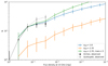 |
Fig. 8. Simulated radio luminosity functions for a 3 Myr old cluster with an initial stellar mass of 104 M⊙, using αIMF = −1.8 and the standard Salpeter value of αIMF = −2.35. |
Following the previous considerations, we proceed to fit cluster models to the observed radio luminosity functions of the Arches and Quintuplet clusters. This is a demonstration of the principle, so we limit ourselves to a crude exploration of parameter space with simple, brute-force Monte Carlo (MC) simulations. To create the MC samples, the observed radio flux densities were varied randomly assuming for each source a Gaussian normal distribution centred on the observed radio flux density and a conservative standard deviation of 30% from the mean value (assuming the same uncertainty for all sources). The parameter space was spanned by two values of αIMF = −1.8, −2.35; ages of 2.5, 3, 3.5, 4, 4.5, and 5 Myr; and cluster masses of 1.0, 1.5, and 2.0 × 10⁴ M⊙.
5.3. Arches cluster
We determined the best fit parameters for each of the 400 MC realisations of the RLF observed by Gallego-Calvente et al. (2021). Figure 9 shows the resulting distribution of the parameters of the best fit models with MIST isochrones and Fig. 10 with Parsec isochrones: Reduced  , αIMF, total cluster mass, and cluster age. There is no clear preference for the total cluster mass, but the top-heavy IMF provides the best solution in the vast majority of cases. The cluster age is broadly distributed, but peaks at 3 to 3.5 Myr, in agreement with the literature.
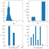 |
Fig. 9. Results of MC simulations of the Arches RLF, using MIST isochrones. |
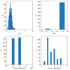 |
Fig. 10. Results of MC simulations of the Arches RLF, using PARSEC isochrones. |
5.4. Quintuplet cluster
We determined the best fit parameters for each of the 400 MC realisations of the RLF observed by us here. Figure 11 shows the resulting distribution of the parameters of the best fit models with MIST isochrones and Fig. 12 for Parsec isochrones. As in the case of the Arches cluster, the cluster mass does not appear to be well constrained, but again the top-heavy IMF provides the best solution in the vast majority of cases. The cluster age is broadly distributed and peaks at 3.5 to 4 Myr, in agreement with literature that assigns an older age to the Quintuplet than to the Arches.
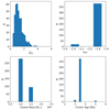 |
Fig. 11. Results of MC simulations of the Quintuplet RLF, using MIST isochrones. |
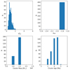 |
Fig. 12. Results of MC simulations of the Quintuplet RLF, using PARSEC isochrones. |
6. Discussion
We fitted very basic models to MC simulations of the Quintuplet and Arches RLFs. These models show that theoretical isochrones appear to provide reasonable matches to the observed RLFs of the two clusters; confirm a top-heavy IMF for the two clusters, which agrees with the conclusions of observational studies of the present-day mass functions of these clusters (Hußmann et al. 2012; Hosek et al. 2019); and cannot provide any significant constraints on the total cluster mass, but indicate roughly the correct ages of the clusters together with the older age of the Quintuplet cluster.
There are important caveats to keep in mind. Above all, not unexpectedly, we find a degree of degeneracy between the IMF slope and the mass of the cluster. Therefore, it is important to constrain the mass and FoV (typically the primary beam of the antennas of the array) of the study. This problem is more complicated due to the uncertain detection limit of our radio observations, which suffer from lower S/N and systematics outside of the centre of the FoV. Finally, mass segregation might have concentrated massive stars near the cluster centre, while three-body interactions may have ejected massive cluster members. All these factors increase the systematic uncertainty of this kind of work. Our next step must consist in improved radio observations of the clusters in order to push down the RLF completeness limit. This can mostly be achieved through a more complete UV coverage of the radio interferometric data by using longer integration times and multi-configuration observations, being sensitive to structures of different angular sizes, to image simultaneously both compact and extended sources. Finally, we can push the radio detections to the limit by keeping in mind that radio stars must necessarily have bright infrared counterparts. These observations will be very relevant for future SKA observations at mid-frequency (SKA-MID), which would permit the study of massive stars and their winds at all stages of evolution up to much lower mass-loss rates, increasing significantly the number of detections.
The NRAO is a facility of the National Science Foundation (NSF) operated under cooperative agreement by Associated Universities, Inc.
Scientists based at the National Radio Astronomical Observatory (NRAO), the European Southern Observatory (ESO), the National Astronomical Observatory of Japan (NAOJ), the Academia Sinica Institute of Astronomy and Astrophysics (ASIAA), the CSIRO division for Astronomy and Space Science (CASS), and the Netherlands Institute for Radio Astronomy (ASTRON) under the guidance of NRAO.
Based on observations made with the NASA/ESA Hubble Space Telescope, obtained from the data archive at the Space Telescope Science Institute. STScI is operated by the Association of Universities for Research in Astronomy, Inc., under NASA contract NAS 5-26555.
Acknowledgments
Karl G. Jansky Very Large Array (JVLA) of the National Radio Astronomy Observatory (NRAO) is a facility of the National Science Foundation (NSF) operated under cooperative agreement by Associated Universities, Inc. A. T. G.-C., R. S., A. A. and B. S. acknowledge financial support from the State Agency for Research of the Spanish MCIU through the “Center of Excellence Severo Ochoa” award for the Instituto de Astrofísica de Andalucía (SEV-2017-0709). A. T. G.-C., R. S., and B. S. acknowledge financial support from national project PGC2018-095049-B-C21 (MCIU/AEI/FEDER, UE). A. A. acknowledges support from national project PGC2018-098915-B-C21 (MCIU/AEI/FEDER, UE). F. N. acknowledges financial support through Spanish grants ESP2017-86582-C4-1-R and PID2019-105552RB-C41 (MINECO/MCIU/AEI/FEDER) and from the Spanish State Research Agency (AEI) through the Unidad de Excelencia “María de Maeztu”-Centro de Astrobiología (CSIC-INTA) project No. MDM-2017-0737. F. N.-L. gratefully acknowledges funding by the Deutsche Forschungsgemeinschaft (DFG, German Research Foundation) – Project-ID 138713538 – SFB 881 (“The Milky Way System”, subproject B8). F.N.-L. acknowledges the sponsorship provided by the Federal Ministry for Education and Research of Germany through the Alexander von Humboldt Foundation. The research leading to these results has received funding from the European Research Council under the European Union’s Seventh Framework Programme (FP7/2007-2013) / ERC grant agreement n° [614922].
References
- Agliozzo, C. 2019, in ALMA2019: Science Results and Cross-Facility Synergies, 66 [Google Scholar]
- Benaglia, P. 2010, in High Energy Phenomena in Massive Stars, eds. J. Martí, P. L. Luque-Escamilla, & J. A. Combi, ASP Conf. Ser., 422, 111 [Google Scholar]
- Bieging, J. H., Abbott, D. C., & Churchwell, E. B. 1989, ApJ, 340, 518 [NASA ADS] [CrossRef] [Google Scholar]
- Bressan, A., Marigo, P., Girardi, L., et al. 2012, MNRAS, 427, 127 [NASA ADS] [CrossRef] [Google Scholar]
- Cappa, C., Goss, W. M., van der Hucht, K. A. 2004, AJ, 127, 2885 [NASA ADS] [CrossRef] [Google Scholar]
- Chen, Y., Girardi, L., Bressan, A., et al. 2014, MNRAS, 444, 2525 [Google Scholar]
- Chen, Y., Bressan, A., Girardi, L., et al. 2015, MNRAS, 452, 1068 [Google Scholar]
- Choi, J., Dotter, A., Conroy, C., et al. 2016, ApJ, 823, 102 [Google Scholar]
- Clark, J. S., Lohr, M. E., Najarro, F., Dong, H., & Martins, F. 2018a, A&A, 617, A65 [NASA ADS] [CrossRef] [EDP Sciences] [Google Scholar]
- Clark, J. S., Lohr, M. E., Patrick, L. R., et al. 2018b, A&A, 618, A2 [NASA ADS] [CrossRef] [EDP Sciences] [Google Scholar]
- Contreras, M. E., Rodriguez, L. F., Gomez, Y., & Velazquez, A. 1996, ApJ, 469, 329 [NASA ADS] [CrossRef] [Google Scholar]
- Dong, H., Wang, Q. D., Cotera, A., et al. 2011, MNRAS, 417, 114 [Google Scholar]
- Dotter, A. 2016, ApJS, 222, 8 [Google Scholar]
- Dzib, S. A., Loinard, L., Rodríguez, L. F., et al. 2017, ApJ, 834, 139 [Google Scholar]
- Figer, D. F., McLean, I. S., & Morris, M. 1999, ApJ, 514, 202 [Google Scholar]
- Gallego-Calvente, A. T., Schödel, R., Alberdi, A., et al. 2021, A&A, 647, A110 [NASA ADS] [CrossRef] [EDP Sciences] [Google Scholar]
- Güdel, M. 2002, ARA&A, 40, 217 [Google Scholar]
- Hosek, Jr., M. W., Lu, J. R., Anderson, J., et al. 2019, ApJ, 870, 44 [NASA ADS] [CrossRef] [Google Scholar]
- Hußmann, B., Stolte, A., Brandner, W., Gennaro, M., & Liermann, A. 2012, A&A, 540, A57 [NASA ADS] [CrossRef] [EDP Sciences] [Google Scholar]
- Lang, C. C., Johnson, K. E., Goss, W. M., & Rodríguez, L. F. 2005, AJ, 130, 2185 [Google Scholar]
- Launhardt, R., Zylka, R., & Mezger, P. G. 2002, A&A, 384, 112 [NASA ADS] [CrossRef] [EDP Sciences] [Google Scholar]
- Leitherer, C., Chapman, J. M., & Koribalski, B. 1995, ApJ, 450, 289 [NASA ADS] [CrossRef] [Google Scholar]
- Leitherer, C., Chapman, J. M., & Koribalski, B. 1997, ApJ, 481, 898 [Google Scholar]
- Liermann, A., Hamann, W. R., & Oskinova, L. M. 2009, A&A, 494, 1137 [NASA ADS] [CrossRef] [EDP Sciences] [Google Scholar]
- Liermann, A., Hamann, W. R., Oskinova, L. M., Todt, H., & Butler, K. 2010, A&A, 524, A82 [NASA ADS] [CrossRef] [EDP Sciences] [Google Scholar]
- Liermann, A., Hamann, W. R., & Oskinova, L. M. 2012, A&A, 540, A14 [NASA ADS] [CrossRef] [EDP Sciences] [Google Scholar]
- Marigo, P., Girardi, L., Bressan, A., et al. 2017, ApJ, 835, 77 [Google Scholar]
- Mason, B. D., Hartkopf, W. I., Gies, D. R., Henry, T. J., & Helsel, J. W. 2009, AJ, 137, 3358 [Google Scholar]
- Montes, G., Pérez-Torres, M. A., Alberdi, A., & González, R. F. 2009, ApJ, 705, 899 [NASA ADS] [CrossRef] [Google Scholar]
- Montes, G., Alberdi, A., Pérez-Torres, M. A., & González, R. F. 2015, Rev. Mex. Astron. Astrofis., 51, 209 [NASA ADS] [Google Scholar]
- Najarro, F., Figer, D. F., Hillier, D. J., Geballe, T. R., & Kudritzki, R. P. 2009, ApJ, 691, 1816 [NASA ADS] [CrossRef] [Google Scholar]
- Najarro, F., Geballe, T. R., Figer, D. F., & de la Fuente, D. 2017, ApJ, 845, 127 [NASA ADS] [CrossRef] [Google Scholar]
- Nogueras-Lara, F., Gallego-Calvente, A. T., Dong, H., et al. 2018, A&A, 610, A83 [NASA ADS] [CrossRef] [EDP Sciences] [Google Scholar]
- Nogueras-Lara, F., Schödel, R., Gallego-Calvente, A. T., et al. 2019a, Nat. Astron., 4, 377 [Google Scholar]
- Nogueras-Lara, F., Schödel, R., Gallego-Calvente, A. T., et al. 2019b, A&A, 631, A20 [NASA ADS] [CrossRef] [EDP Sciences] [Google Scholar]
- Nogueras-Lara, F., Schödel, R., & Neumayer, N. 2021, A&A, 653, A133 [NASA ADS] [CrossRef] [EDP Sciences] [Google Scholar]
- Pastorelli, G., Marigo, P., Girardi, L., et al. 2019, MNRAS, 485, 5666 [Google Scholar]
- Pastorelli, G., Marigo, P., Girardi, L., et al. 2020, MNRAS, 498, 3283 [Google Scholar]
- Paxton, B., Bildsten, L., Dotter, A., et al. 2011, ApJS, 192, 3 [Google Scholar]
- Paxton, B., Cantiello, M., Arras, P., et al. 2013, ApJS, 208, 4 [Google Scholar]
- Paxton, B., Marchant, P., Schwab, J., et al. 2015, ApJS, 220, 15 [Google Scholar]
- Perley, R. A., & Butler, B. J. 2013, ApJS, 204, 19 [Google Scholar]
- Reid, M. J., Schneps, M. H., Moran, J. M., et al. 1988, ApJ, 330, 809 [Google Scholar]
- Rui, N. Z., Hosek, Jr., M. W., Lu, J. R., et al. 2019, ApJ, 877, 37 [NASA ADS] [CrossRef] [Google Scholar]
- Sana, H., & Evans, C. J. 2011, in IAU Symposium, eds. C. Neiner, G. Wade, G. Meynet, & G. Peters, IAU Symp., 272, 474 [NASA ADS] [Google Scholar]
- Sanchez-Bermudez, J., Alberdi, A., Schödel, R., et al. 2019, A&A, 624, A55 [EDP Sciences] [Google Scholar]
- Schneider, F. R. N., Izzard, R. G., de Mink, S. E., et al. 2014, ApJ, 780, 117 [Google Scholar]
- Scuderi, S., Panagia, N., Stanghellini, C., Trigilio, C., & Umana, G. 1998, A&A, 332, 251 [NASA ADS] [Google Scholar]
- Sota, A., Maíz Apellániz, J., Morrell, N. I., et al. 2014, ApJS, 211, 10 [Google Scholar]
- Tang, J., Bressan, A., Rosenfield, P., et al. 2014, MNRAS, 445, 4287 [NASA ADS] [CrossRef] [Google Scholar]
- Umana, G., Trigilio, C., Cerrigone, L., et al. 2015, in Advancing Astrophysics with the Square Kilometre Array (AASKA14), 118 [CrossRef] [Google Scholar]
Appendix A: Additional tables
JVLA flux densities of the compact sources of the Quintuplet cluster from these observations.
Radio mass-loss rates in the C-band epoch (2018) and in the two X-band epochs (2016, 2018).
All Tables
JVLA flux densities of the compact sources of the Quintuplet cluster from these observations.
Radio mass-loss rates in the C-band epoch (2018) and in the two X-band epochs (2016, 2018).
All Figures
|
Fig. 1. JHK false colour image of the Quintuplet cluster from the GALACTICNUCLEUS survey. Credits: Nogueras-Lara et al. (2018,2019b). |
| In the text | |
|
Fig. 2. Detected point sources above 5σ at 10 GHz and 6 GHz. Top: closeup of the Quintuplet cluster from the 2016 X-band image corrected for primary-beam attenuation. The clean beam is 0.47″ × 0.15″, PA = 25.29°. The off-source rms noise level is 4.3 μJy beam−1. The contour levels represent −1, 1, 2, 3, 4, 5, and 6 times 5 σ. Bottom: closeup of the Quintuplet cluster showing most of the detected sources from the 2018 C-band image corrected for primary-beam attenuation. The resolution is 0.62″ × 0.21″, PA = 19.97°. The off-source rms noise level is 6.6 μJy beam−1. The contour levels represent −1, 1, 2, 3, 4, 5, and 6 times 5 σ. |
| In the text | |
|
Fig. 3. HST/WFC3 F153M image of the Quintuplet cluster with identified radio stars labelled. |
| In the text | |
|
Fig. 4. Composition of the HST/WFC3 F153M image from HST archive with a Paschen α image by Dong et al. (2011). Blue: HST WFC3 F153M; Red: HST NIC3 Paschen α. The QR1−3 sources by Lang et al. (2005) are encircled. |
| In the text | |
|
Fig. 5. Histogram of Sν of observed radio stars in Arches cluster. Blue solid histogram: Observed flux densities of radio stars in the Arches cluster (Gallego-Calvente et al. 2021). Orange outline: Radio fluxes of the same stars, using the mass-loss rates reported by Gallego-Calvente et al. (2021) and converting to radio flux density with Eq. (1) assuming the same parameters for all stars. |
| In the text | |
|
Fig. 6. Radio flux densities of massive stars in a model cluster, using MIST isochrones. Top: present-day mas function. Middle: histograms of predicted radio flux densities. Bottom: cumulative histograms of predicted radio flux densities. The black histogram corresponds to the observed data for the Arches cluster (Gallego-Calvente et al. 2021, dotted) and the grey histogram to the observed data for the Quintuplet cluster (this work, solid). |
| In the text | |
|
Fig. 7. Radio flux densities of massive stars in a model cluster, using PARSEC isochrones. Top: present-day mas function. Middle: histograms of predicted radio flux densities. Bottom: cumulative histograms of predicted radio flux densities. The black histogram corresponds to the observed data for the Arches cluster (Gallego-Calvente et al. 2021, dotted) and the grey histogram to the observed data for the Quintuplet cluster (this work, solid). |
| In the text | |
|
Fig. 8. Simulated radio luminosity functions for a 3 Myr old cluster with an initial stellar mass of 104 M⊙, using αIMF = −1.8 and the standard Salpeter value of αIMF = −2.35. |
| In the text | |
|
Fig. 9. Results of MC simulations of the Arches RLF, using MIST isochrones. |
| In the text | |
|
Fig. 10. Results of MC simulations of the Arches RLF, using PARSEC isochrones. |
| In the text | |
|
Fig. 11. Results of MC simulations of the Quintuplet RLF, using MIST isochrones. |
| In the text | |
|
Fig. 12. Results of MC simulations of the Quintuplet RLF, using PARSEC isochrones. |
| In the text | |
Current usage metrics show cumulative count of Article Views (full-text article views including HTML views, PDF and ePub downloads, according to the available data) and Abstracts Views on Vision4Press platform.
Data correspond to usage on the plateform after 2015. The current usage metrics is available 48-96 hours after online publication and is updated daily on week days.
Initial download of the metrics may take a while.