| Issue |
A&A
Volume 692, December 2024
|
|
|---|---|---|
| Article Number | A23 | |
| Number of page(s) | 13 | |
| Section | Galactic structure, stellar clusters and populations | |
| DOI | https://doi.org/10.1051/0004-6361/202451771 | |
| Published online | 02 December 2024 | |
A multi-frequency, multi-epoch radio continuum study of the Arches cluster with the Very Large Array
1
Instituto de Astrofísica de Andalucía (CSIC), Glorieta de la Astronomía s/n,
18008
Granada,
Spain
2
School of Sciences, European University Cyprus,
Diogenes street, Engomi,
1516
Nicosia,
Cyprus
3
Centro de Astrobiología, CSIC-INTA,
Ctra de Torrejón a Ajalvir km 4,
28850
Torrejón de Ardoz, Madrid,
Spain
4
Universitat de València. Departament d’Astronomia i Astrofísica. Facultat de Física.
Av. Doctor Moliner, 50 -
Burjassot,
Valencia
★ Corresponding author; This email address is being protected from spambots. You need JavaScript enabled to view it.
Received:
2
August
2024
Accepted:
21
October
2024
Abstract
Context. The Arches cluster, one of the most massive clusters in the Milky Way, is located about 30 pc in projection from the central massive black hole Sagittarius A* at a distance of ≈8 kpc from Earth. With its high mass, young age, and location in the Galaxy’s most extreme star forming environment, the Arches is an extraordinary laboratory for studying massive stars and clusters.
Aims. Our objective is to improve our knowledge of the properties of massive stars and the Arches cluster through high-angular-resolution radio continuum studies.
Methods. We observed the Arches cluster with the Karl G. Jansky Very Large Array in the C- and X-bands (central frequencies of 6 and 10 GHz respectively) in two epochs at C-band and five epochs at X-band throughout 2016, 2018, and 2022, covering time spans ranging from 22 days to 6 years. We used the A-configuration to achieve the highest possible angular resolution and cross-matched the detected point-sources with stars detected in the infrared, using proper motion catalogues to ensure cluster membership.
Results. We report the most extensive radio point-source catalogue of the cluster to date, with a total of 25 radio detections (7 more than the most recent study). We also created the deepest (2.5 μJy in X-band) images of the cluster so far in the 4 to 12 GHz frequency range. Most of our stellar radio sources (12 out of 18) show a positive spectral index, indicating that the dominant emission process is free-free thermal radiation, which probably originates from stellar winds. We find that radio variability is more frequent than what was inferred from previous observations, and affects up to 60% of the sources associated with bright stellar counterparts, with two of them, F18 and F26, showing extreme flux variability. We propose four of our detections (F6, F18, F19, and F26) as primary candidates for colliding-wind binaries (CWBs) based on their consistent flat-to-negative spectral index. We classify F7, F9, F12, F14, and F55 as CWB binary candidates based on their high flux and/or spectral index variability, and X-ray counterparts. Thus, we infer a 14/23 ≈ 61% multiplicity fraction for the radio stars of the Arches cluster when combining our findings with recent infrared radial velocity studies.
Key words: stars: massive / Galaxy: center / open clusters and associations: individual: Arches cluster / radio continuum: stars
© The Authors 2024
 Open Access article, published by EDP Sciences, under the terms of the Creative Commons Attribution License (https://creativecommons.org/licenses/by/4.0), which permits unrestricted use, distribution, and reproduction in any medium, provided the original work is properly cited.
This article is published in open access under the Subscribe to Open model. This email address is being protected from spambots. You need JavaScript enabled to view it. to support open access publication.
1 Introduction
Young massive star clusters (YMCs) are targets of great interest in astrophysics. They can host from dozens to well over a hundred massive (≳10 M⊙) early-type stars, which dramatically affect their environment with their intense UV radiation, strong stellar winds, and dramatic demise as supernovae. As massive stars are short-lived, there are only a handful of known YMCs with masses above ~104 M⊙ in the Milky Way, all of them located several kiloparsecs (kpc) from Earth. Regarding extragalactic YMCs beyond the Milky Way and the Magellanic Clouds, their individual members cannot be easily separated and are much fainter than their Galactic counterparts. The Galactic centre (GC; at a distance of ≈8 kpc, GRAVITY Collaboration 2019) is host to three YMCs: the Arches (Figer et al. 2002) and Quintuplet clusters (Figer et al. 1999), and the 104 M⊙ of young massive stars within 0.5 pc of the supermassive black hole (von Fellenberg et al. 2022; Lu et al. 2013). Arches and Quintuplet are located around 30 pc in projection from Sgr A*, within the so-called central molecular zone (CMZ), the turbulent inner R ~ 100 pc of the Milky Way (Henshaw et al. 2023). Both clusters are around 2–5 Myr old, with masses of a few 104 M⊙ (Najarro et al. 2004; Martins et al. 2008; Liermann et al. 2012; Clark et al. 2018a,b).
The CMZ contains 3–10% of the molecular gas in the Milky Way, despite occupying ≤0.01% of its volume. The GC is the most prolific star forming region in the entire Galaxy and may be considered a local analogue of high-redshift starburst galaxies (Kruijssen & Longmore 2013). Our position within the Galactic disc makes the GC an extremely extinguished target (AV ~ 30 mag; e.g. Nishiyama et al. 2008; Nogueras-Lara et al. 2020). Thus, studies of the Arches and Quintuplet clusters are limited to the radio, infrared, and X-ray frequency domains (e.g. Gallego-Calvente et al. 2021; Clark et al. 2018a; Muno et al. 2009).
Radio emission from massive stars is associated with their strong ionised winds. There are two main non-exclusive emission mechanisms that cause radio emission from massive stars in the few GHz range. On the one hand, thermal free-free radiation is emitted by the so-called line-driven ionised winds of massive stars (Castor et al. 1975; Abbott 1980), while on the other, in a system of massive binaries, non-thermal synchrotron emission may arise from the so-called colliding-wind region between the stars. In order for this non-thermal emission to dominate over the free-free radiation arising from the winds of each star, the orbital separation must be sufficiently large (periods of more than a few weeks); otherwise, the synchrotron emission will be absorbed within the optically thick area of the colliding-wind region, thus masking the observational traces of binarity (De Becker 2007; Sanchez-Bermudez et al. 2019). Therefore, only a subset of all colliding-wind binaries (CWBs) present observable traces of a particle-accelerating mechanism, which is considered to be the main mechanism driving non-thermal emission in massive stars (De Becker 2007; De Becker & Raucq 2013).
With multi-frequency radio observations, we can measure the spectral index of a particular source, obtaining insight into its physical nature. Assuming a dependence of flux density with frequency of the form Sν ∝ να, where α is the spectral index, we can discriminate between thermal (free-free) and non-thermal (synchrotron) emission. The former is characterised by a positive spectral index (assuming a spherically symmetric, homogeneous wind arising from a single star: α ≈ 0.6 Wright & Barlow 1975). The latter is associated with a significantly lower spectral index (α ≲ 0.0, De Becker 2007). Furthermore, multi-epoch observations can provide information as to the orbital phase of a multiple system by offering means to study changes in the spectral index of a particular radio star (Dougherty et al. 2005; Sanchez-Bermudez et al. 2019). Highly eccentric systems, such as those purportedly hosted by the Arches cluster (Clark et al. 2023), can be especially prone to spectral index variability.
Deviations from the α ≈ 0.6 canonical value for free-free thermal emission are expected and can be caused by wind clumping and flares, a thermal contribution from a short-period CWB, or a contribution from non-thermal radiation within the colliding-wind region of a binary system. However, thermal radio emission arising from stable, fully ionised, isolated stars is not expected to display relevant flux variability on timescales shorter than the star’s evolutionary timescale, with the exception of the luminous blue variable phase. Therefore, radio variability may be an indirect indicator of a non-negligible, non-thermal component in the observed radio emission (De Becker & Raucq 2013) or (less likely in the case of Wolf-Rayet stars) of an eruptive mass-loss episode.
Massive stars are scarce and are located at relatively large (kpc) distances. Thus, the study of massive stellar evolution – especially the post main-sequence phase – is an area of ongoing development, both theoretical and observational (e.g. Andrews et al. 2019; Björklund et al. 2023; Toalá et al. 2024). We can use radio observations to detect free-free emission arising from the stellar winds of massive stars. This emission is sensitive to massloss, which plays a crucial role in their evolutionary pathway and can contain information about wind variability, geometry (clumping), and flaring events. As previously mentioned, evidence of non-thermal radio emission is a well-established indicator of multiplicity (De Becker & Raucq 2013), making radio continuum observations a complementary approach to spectroscopic studies of the binary fraction of massive stars. Moreover, whereas spectroscopic studies are more sensitive to short-period binaries (periods of a few days), non-thermal emission traces multiplicity in regions of the orbital parameter space that may not be available to radial velocity studies given the limited length of the spectroscopic campaigns themselves. In addition, non-thermal emission is not affected by the orbital inclination of the system with respect to the line of sight, which is an important bias to take into account in spectroscopic studies.
In our previous work (Gallego-Calvente et al. 2021), we studied the radio emission from the stars of the Arches cluster with the aim of establishing constraints on the properties of cluster members with radio observations only. With a relatively limited time span (only two observational epochs at our disposal: 2016 and 2018), and with most of the observations carried out at one band (X-band), our variability, spectral index, and massloss rate analyses were incomplete. In the present work, we build on our previous results by incorporating new multi-wavelength observations and proper motion measurements, quantitatively improving our variability, mass-loss, and spectral index analyses. This paper is structured as follows: Section 2 describes the data reduction and imaging process. In Sect. 3, we show how we extracted and analysed flux densities, source positions, and spectral indices, and present the main results of our study. Finally, in Sect. 4, we discuss our results and in Sect. 5 we summarise our conclusions.
2 Observations and imaging
We observed the Arches cluster (pointing position of αJ2000 = 17h45m50.49s, δJ2000 = −28°49′19.92″) with the Karl G. Jansky Very Large Array (VLA) in A-configuration in the C- and X-bands (central frequencies of 6 and 10 GHz respectively, both with a total bandwidth of 4 GHz and 3-bit sampling). Our seven observations were carried out in three different years: 2016, 2018 and 2022; see Table A.1 for details.
We used CASA 6.4.1 (Common Astronomy Software Applications, CASA Team et al. 2022) with the pipeline version 2022.2.0.64, and performed a standard continuum calibration of the data. We also calibrated our data manually for comparison, but the results in terms of point-source flux extraction and image quality were extremely similar. The data from 2016 and 2018 are identical to those described in Gallego-Calvente et al. (2021), but we re-reduced and calibrated the raw data again (see Sect. 4.1). We used 3C286 (J1331+3030) as the flux and bandpass calibrator for all observations. For the 2016 and 2018 observations, we used J1744–3116 as the phase calibrator, whereas we used J1820–2528 for 2022. This change was made because J1744–3116 showed some extended emission in A-configuration, but it did not result in any systematic flux difference between 2016, 2018, and 2022. As our main goal is to study radio point-sources, we reduced the contribution of the extended emission present in our field (see e.g. Lang et al. 2005; Heywood et al. 2022) by performing u-v cuts of 100 kλ and 150 kλ for the C- and X-bands, respectively. This enabled us to severely diminish the contribution of the extended emission present in the radio-bright zone of the GC; although this contribution was not fully removed, and some areas near the cluster core are still affected by it. This mainly results in higher rms noise in this particular region, especially in C-band.
We performed phase-only self-calibration for each individual observation, as well as for the combined data. We combined polarisations and spectral windows in order to achieve sufficient signal-to-noise ratios (S/N) in the self-calibration solutions. The optimal solution intervals (≲5% solutions with S/N < 5) range from 20 s to 30 s for all our observations. For the concatenated data of 2016 and 2022, we used the largest solution interval of the individual observations composing them. We used the aforementioned u-v cut to compute the self-calibration solutions with the gaincal task and to perform the subsequent imaging. We note that amplitude self-calibration did not improve the image quality or flux extraction in any significant way. Indeed, enforcing amplitude self-calibration incremented the total amount of flagged visibilities, which resulted in a poorer image quality, especially around the phase centre, and so we discarded that approach.
We deconvolved the images with the CLEAN algorithm (Högbom 1974) – implemented in the CASA task tclean. We used 4 pixels across the synthesised beam FWHM, which resulted in pixel sizes of ![Mathematical equation: $\[0^{\prime\prime}_\cdot 0825\]$](/articles/aa/full_html/2024/12/aa51771-24/aa51771-24-eq1.png) and
and ![Mathematical equation: $\[0^{\prime\prime}_\cdot 05\]$](/articles/aa/full_html/2024/12/aa51771-24/aa51771-24-eq2.png) for the C- and X-band images respectively. Although the VLA primary beam’s FWHM (in arcminutes) is ≈42 × (1 GHz/ν), for this work, we mainly focused on the 1′ × 1′ area centred on the Arches cluster, so that we covered the entire massive star catalogue of Clark et al. (2018a). We tried different weightings: natural, uniform, and Briggs with several robust parameters. We obtained the best results with Briggs weighting and a robust parameter of 0.5 in terms of point-source sensitivity, resolution, and rms noise. The gain parameter was set to 0.05 as in Gallego-Calvente et al. (2021) to facilitate spotting and masking of the faintest sources during the interactive cleaning. We imposed an rms-based stopping criterion of 5σ for all images. Table A.1 provides a list of the beam geometry and rms noise reached in all images.
for the C- and X-band images respectively. Although the VLA primary beam’s FWHM (in arcminutes) is ≈42 × (1 GHz/ν), for this work, we mainly focused on the 1′ × 1′ area centred on the Arches cluster, so that we covered the entire massive star catalogue of Clark et al. (2018a). We tried different weightings: natural, uniform, and Briggs with several robust parameters. We obtained the best results with Briggs weighting and a robust parameter of 0.5 in terms of point-source sensitivity, resolution, and rms noise. The gain parameter was set to 0.05 as in Gallego-Calvente et al. (2021) to facilitate spotting and masking of the faintest sources during the interactive cleaning. We imposed an rms-based stopping criterion of 5σ for all images. Table A.1 provides a list of the beam geometry and rms noise reached in all images.
Furthermore, we obtained deep radio images for each band by combining all visibilities of a given band using the CASA task concat. After concatenation, we performed global phaseonly self-calibration in order to align all sources. To this end, we used one solution interval per scan. Figure 1 shows the deep X-band image of the cluster along the detected sources (see Sect. 3.2).
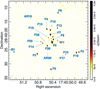 |
Fig. 1 Deep X-band image of the Arches cluster (see Table A.1 for details). Sources are labelled with the NIR stellar ID from Clark et al. (2018a) with the exception of the AR19 and AR20 sources (see Sect. 3.2). |
3 Analysis and results
3.1 Flux extraction and astrometry
We used the CASA task imfit to extract point-source fluxes, positions, and their related uncertainties (Condon 1997). Briefly, this task fits a single 2D Gaussian to the emission lying within a given region, which is provided by the user as input. We used circular regions with ![Mathematical equation: $\[1^{\prime\prime}_\cdot 5\]$](/articles/aa/full_html/2024/12/aa51771-24/aa51771-24-eq3.png) diameter so that a sufficiently large area was covered for local rms computation during the fit. We made sure the resulting fits were similar in shape to the synthesised beam geometry of each image. In some particularly faint cases (such as F55; see Sect. 3.2) that did not match the beam shape (especially for some sources near the cluster core at C-band, which is more prominently affected by the non-thermal extended emission), the peak flux was used instead of the integrated flux. Increasing the region size in imfit did not result in a significant difference in fluxes and their uncertainties. In addition to the flux error returned by the imfit task, we quadratically added systematic flux errors of 3 and 5% due to absolute calibration for the X- and C-band, respectively (Perley & Butler 2017).
diameter so that a sufficiently large area was covered for local rms computation during the fit. We made sure the resulting fits were similar in shape to the synthesised beam geometry of each image. In some particularly faint cases (such as F55; see Sect. 3.2) that did not match the beam shape (especially for some sources near the cluster core at C-band, which is more prominently affected by the non-thermal extended emission), the peak flux was used instead of the integrated flux. Increasing the region size in imfit did not result in a significant difference in fluxes and their uncertainties. In addition to the flux error returned by the imfit task, we quadratically added systematic flux errors of 3 and 5% due to absolute calibration for the X- and C-band, respectively (Perley & Butler 2017).
In a radio-interferometer, astrometric information is encoded in the phases. As the data were self-calibrated in phases, absolute astrometric information was lost and we found systematic coordinate offsets between all our observations. We referred all individual images to our deep X-band image, given that the position uncertainties returned by the imfit task depend in part on the S/N of a given detection, and the deep X-band image shows the best off-source rms noise of all our images. Once the coordinates of each individual observation were referenced to our deep X-band image, we used the Arches stellar catalogue provided by Hosek et al. (2022) to establish the astrometric reference frame. After correcting for an initial coordinate offset, our sources are cross-matched with their cluster members (Pclust > 0.7) within a median ![Mathematical equation: $\[0^{\prime\prime}_\cdot0003 \pm0^{\prime\prime}_\cdot0039\]$](/articles/aa/full_html/2024/12/aa51771-24/aa51771-24-eq4.png) in Right Ascension (RA) and
in Right Ascension (RA) and ![Mathematical equation: $\[-0^{\prime\prime}_\cdot001 \pm0^{\prime\prime}_\cdot013\]$](/articles/aa/full_html/2024/12/aa51771-24/aa51771-24-eq5.png) in Declination (Dec). The uncertainties represent the standard deviation of the previous offsets. Once we cross-matched our sources, all coordinate uncertainties were combined with the following expression:
in Declination (Dec). The uncertainties represent the standard deviation of the previous offsets. Once we cross-matched our sources, all coordinate uncertainties were combined with the following expression:
![Mathematical equation: $\[\sigma_{\mathrm{pos}}=\sqrt{\sigma_{\mathrm{fit}}^{2}+\sigma_{\mathrm{std}}^{2}+\sigma_{\theta}^{2}}\]$](/articles/aa/full_html/2024/12/aa51771-24/aa51771-24-eq6.png) (1)
(1)
where σfit is the positional uncertainty returned by the fit in our deep X-band image, σstd is the previously mentioned standard deviation of the offsets with respect to Hosek et al. (2022), and ![Mathematical equation: $\[\sigma_{\theta}=r_{\theta} \times \frac{\nu_{c}}{\nu_{0}}\]$](/articles/aa/full_html/2024/12/aa51771-24/aa51771-24-eq7.png) is a factor that takes into account the channel width (vc = 2000 kHz), central frequency (v0 = 10 GHz), and rθ, which is the distance of a given source from the phase centre (Thompson et al. 2017).
is a factor that takes into account the channel width (vc = 2000 kHz), central frequency (v0 = 10 GHz), and rθ, which is the distance of a given source from the phase centre (Thompson et al. 2017).
We present the most complete radio point-source catalogue and the deepest radio images (in the few GHz range) of the Arches cluster to date. Flux densities, positions, and their related uncertainties can be found in Table A.2.
3.2 Cross-matching with stars
We found a systematic coordinate offset of ≈1″ between our deep X-band detections and the Clark et al. (2018a) stellar catalogue. We computed median offsets of ![Mathematical equation: $\[-0^{\prime \prime}_\cdot 92 \pm 0^{\prime \prime}_\cdot03\]$](/articles/aa/full_html/2024/12/aa51771-24/aa51771-24-eq8.png) in RA and
in RA and ![Mathematical equation: $\[0^{\prime \prime}_\cdot 483 \pm 0^{\prime \prime}_\cdot008\]$](/articles/aa/full_html/2024/12/aa51771-24/aa51771-24-eq9.png) in Dec. between our bright (>0.1 mJy), isolated deep X-band detections and the near-infrared (NIR) sources from Clark et al. (2018a). The errors represent the standard deviation of the offsets. After correcting for the offsets, radio-NIR cross-matching was performed using a search radius of
in Dec. between our bright (>0.1 mJy), isolated deep X-band detections and the near-infrared (NIR) sources from Clark et al. (2018a). The errors represent the standard deviation of the offsets. After correcting for the offsets, radio-NIR cross-matching was performed using a search radius of ![Mathematical equation: $\[0^{\prime \prime}_\cdot 2\]$](/articles/aa/full_html/2024/12/aa51771-24/aa51771-24-eq10.png) around all our radio sources. Additionally, we used the HST Paschen-α catalogue from Dong et al. (2011) for the case of two radio sources with clear stellar counterparts that are not included in Clark et al. (2018a). In total, 23 out of the 25 point-sources in the deep X-band image have bright stellar counterparts. The first column of Table A.2 shows the NIR stellar identification of our radio point-sources, and Fig. 1 labels these sources in the deep X-band image.
around all our radio sources. Additionally, we used the HST Paschen-α catalogue from Dong et al. (2011) for the case of two radio sources with clear stellar counterparts that are not included in Clark et al. (2018a). In total, 23 out of the 25 point-sources in the deep X-band image have bright stellar counterparts. The first column of Table A.2 shows the NIR stellar identification of our radio point-sources, and Fig. 1 labels these sources in the deep X-band image.
3.3 Variability assessment
For a given detection and for each band, we followed a similar procedure to the one described in Zhao et al. (2020, see their Appendix A1) to quantify radio-variability. We identified a particular source as variable if it met the following criteria:
![Mathematical equation: $\[\sigma_{\mathrm{VAR}}=\frac{S_{\nu}^{\max }-S_{\nu}^{\min }}{\left(\sum_{i}^{N} \frac{1}{\sigma_{S_{i}}^{2}}\right)^{-1 / 2}}>5\]$](/articles/aa/full_html/2024/12/aa51771-24/aa51771-24-eq11.png) (2)
(2)
where ![Mathematical equation: $\[S_{\nu}^{\max }\]$](/articles/aa/full_html/2024/12/aa51771-24/aa51771-24-eq12.png) and
and ![Mathematical equation: $\[S_{\nu}^{\min }\]$](/articles/aa/full_html/2024/12/aa51771-24/aa51771-24-eq13.png) are, respectively, the maximum and minimum flux density values of a particular source at a given frequency ν, N is the number of observations in which a given source is detected, and
are, respectively, the maximum and minimum flux density values of a particular source at a given frequency ν, N is the number of observations in which a given source is detected, and ![Mathematical equation: $\[\sigma_{S_{i}}\]$](/articles/aa/full_html/2024/12/aa51771-24/aa51771-24-eq14.png) is the flux density uncertainty of that source in the i-eth observation. Therefore, we computed σVAR using five and two individual X- and C-band observations, respectively. We note that, as the absolute systematic error due to absolute calibration affects all sources equally for a given band, we excluded it from the variability analysis. Using individual observations only allows us to measure the brightest sources. In order to obtain variability data for the faintest radio detections, we performed an analogous assessment with the combined 2016 and 2022 X-band images. Thus, we computed σVAR for 23 radio stars, out of which 13 are noted as variables with this approach.
is the flux density uncertainty of that source in the i-eth observation. Therefore, we computed σVAR using five and two individual X- and C-band observations, respectively. We note that, as the absolute systematic error due to absolute calibration affects all sources equally for a given band, we excluded it from the variability analysis. Using individual observations only allows us to measure the brightest sources. In order to obtain variability data for the faintest radio detections, we performed an analogous assessment with the combined 2016 and 2022 X-band images. Thus, we computed σVAR for 23 radio stars, out of which 13 are noted as variables with this approach.
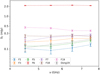 |
Fig. 2 Flux versus frequency plot in logarithmic space in the case of the C-band observations from 10 June 2018. |
3.4 Spectral indices
We derived the spectral indices of our radio stars using two different approaches. First, we divided the visibilities of each observation into four bandwidth chunks. Thus, we obtained four sub-images of 1 GHz bandwidth each. After measuring the fluxes of the sources in the sub-images, the spectral index of each source was computed via a least-squares linear fit with an inverse variance weighting in logarithmic space (see Fig. 2). In order for a spectral index to be computed this way, a source needed to be detected in all 1 GHz bandwidth images (minimum of four points for the linear fit). Furthermore, in the case of the C- and X-band observations carried out during 4 July 2022, we combined both measurement sets with the task concat and proceeded analogously. This resulted in a dataset with a broader bandwidth, ranging from 4 to 12 GHz, and thus a total of eight images of 1 GHz each, as well as a total of eight points to be fitted with the weighted least-squares method.
We took into account both the fitting error returned by imfit and the previously mentioned error due to absolute calibration when setting the weights of the least-squares fit.
Subsequently, for those sources that were too faint to be fitted in the sub-images, but were detected in both bands for a given year (2018 or 2022), we derived their spectral index as follows:
![Mathematical equation: $\[\alpha=\frac{\log \left(S_{~C} / S_{~X}\right)}{\log \left(v_{C} / v_{X}\right)}\]$](/articles/aa/full_html/2024/12/aa51771-24/aa51771-24-eq15.png) (3)
(3)
and their related uncertainties through conventional error propagation:
![Mathematical equation: $\[\sigma_{\alpha}=\frac{1}{\log \left(\nu_{C} / \nu_{X}\right)} \times \sqrt{\left(\frac{\sigma_{S_{~C}}}{S_{~C}}\right)^{2}+\left(\frac{\sigma_{S_{~X}}}{S_{~X}}\right)^{2}}\]$](/articles/aa/full_html/2024/12/aa51771-24/aa51771-24-eq16.png) (4)
(4)
where Sv and ![Mathematical equation: $\[\sigma_{S_{\nu}}\]$](/articles/aa/full_html/2024/12/aa51771-24/aa51771-24-eq17.png) are, respectively, the flux and flux error of a particular source for a given frequency ν, and νC and νX are the central frequencies of the C- and X-bands (6 and 10 GHz, respectively). We note that, if we use the latter method, as the C- and X-band 2018 observations were carried out two months apart, we must consider the possibility of source variability within this time span. If that were the case, the spectral index derived from this pair of observations would not be reliable. To address this issue, we used the two pairs of X-band observations from 2016 and 2022, which were taken a few months apart, and performed the same variability analysis described in Sect. 3.3. Thus, we found that two sources, F6 and F18, exhibit significant variability on a timescale of a few months. This makes their 2018 spectral indices derived with Eqs. (3) and (4) unreliable.
are, respectively, the flux and flux error of a particular source for a given frequency ν, and νC and νX are the central frequencies of the C- and X-bands (6 and 10 GHz, respectively). We note that, if we use the latter method, as the C- and X-band 2018 observations were carried out two months apart, we must consider the possibility of source variability within this time span. If that were the case, the spectral index derived from this pair of observations would not be reliable. To address this issue, we used the two pairs of X-band observations from 2016 and 2022, which were taken a few months apart, and performed the same variability analysis described in Sect. 3.3. Thus, we found that two sources, F6 and F18, exhibit significant variability on a timescale of a few months. This makes their 2018 spectral indices derived with Eqs. (3) and (4) unreliable.
Table 1 shows the spectral indices of our radio stars. In this table, the columns denoted ![Mathematical equation: $\[\alpha_{[\mathrm{band}]}^{[\mathrm{DD} /\mathrm{MM} / \mathrm{YY}]}\]$](/articles/aa/full_html/2024/12/aa51771-24/aa51771-24-eq24.png) correspond to the spectral indices derived from the least-squares method and those columns denoted α[year] correspond to the values obtained from the error propagation method using Eqs. (3) and (4).
correspond to the spectral indices derived from the least-squares method and those columns denoted α[year] correspond to the values obtained from the error propagation method using Eqs. (3) and (4).
In a similar way to the flux densities, we searched for significant changes in α throughout our observations. To this end, we computed the following quantity:
![Mathematical equation: $\[\Xi=\frac{\left|\alpha_{i}-\alpha_{j}\right|}{\left(\frac{1}{\mathrm{e} \alpha_{i}^{2}}+\frac{1}{\mathrm{e} \alpha_{j}^{2}}\right)^{-1 / 2}}\]$](/articles/aa/full_html/2024/12/aa51771-24/aa51771-24-eq25.png) (5)
(5)
where the sub-indices i, j represent the two different observations in each year, and eαi,j denotes their respective spectral index uncertainties. We refer to Sect. 4.2 for further discussion of the Ξ values obtained for our radio detections.
Spectral indices.
3.5 Proper motions and cluster membership
We used the proper motion catalogue by Hosek et al. (2022) (Arches absolute proper motions of μα cos δ =-0.80 ± 0.032 mas yr−1 and μδ = −1.89 ± 0.021 mas yr−1) to ensure cluster membership of our radio point-sources. Proper motions, as well as the cluster membership probability from their work are listed in Table 2 along with the corresponding NIR stellar ID.
With these results, we could confirm that Dong 19 and Dong96 are bona fide cluster members. Therefore, we included them in our analysis, despite them being separated by ≈30″ and ≈50″ from the cluster core, respectively. Figure 3 shows the positions of the two sources with respect to the Arches.
Table 2 also shows relatively low cluster membership probabilities for some of our detections; for example, F7. We note that Hosek et al. (2022) cluster membership probability is based on a proper motion-only Bayesian analysis, but we also considered detections close to the Arches core as cluster members because the possibility of random chance alignment between an isolated massive star and the cluster core is low (e.g. Clark et al. 2021).
Proper motions and cluster membership probability.
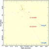 |
Fig. 3 Positions of Dong19 and Dong96 with respect to the cluster core. |
4 Discussion
4.1 Comparison with the pilot study
As explained in Sect. 2, for the sake of consistency, we decided to reduce all data, including those from 2016 and 2018, using the same version of the VLA pipeline. Our study presents two major improvements with respect to the pilot study of Gallego-Calvente et al. (2021). Firstly, while re-reducing the 2016 and 2018 data, we were able to achieve self-calibration, which drastically improved image quality. This resulted in more accurate flux extraction and better uncertainties, especially around the central, brightest source F6. Secondly, the addition of the 2022 data provided us with a longer temporal baseline wit which to asses variability, as well as another measurement of the spectral index and the deepest X-band images of any year. Also, the Hosek et al. (2022) proper motion study allowed us to confirm Dong 19 and Dong96 as cluster members based on their Bayesian analysis. Collectively, this led to the detection of 25 radio sources, which is 7 more than in Gallego-Calvente et al. (2021), as well as an expansion upon their variability analysis, in which they find that ≲15% of their sources are variable, strongly contrasting with the variability fraction we find, of ≲60%. Also, we did not have to correct for the factor ~2 offset between the 2016 and 2018 X-band observations as done by Gallego-Calvente et al. (2021), because we detected no systematic offset between these years. Finally, our approach to spectral index computation discussed in Sect. 3.4 allowed us to study the spectral behaviour of our radio stars at all the observed epochs, improving the spectral index uncertainties by a factor of between 2 and 3, especially for the brightest sources, which is relevant to the determination of spectral index variability, its possible correlation with flux density variability, and any potential connection with the phase of a multiple system.
4.2 Spectral index variability
Significant changes of the spectral index might be an indicator of changes in the relative weights of free-free and non-thermal emission, of an eruptive mass-loss episode, or of clumping and porosity in the stellar winds. Figure 4 shows the Ξ value from Eq. (5) as a function of mean spectral index. We classified sources as non-thermal if they showed negative or flat spectral indices consistently throughout our observations, and thermal sources as those with consistent positive α values throughout all epochs.
We set a threshold at Ξ > 5, as we did with flux variability, and we can see from Fig. 4 that, when compared to thermal radio stars, non-thermal sources are more likely to showcase spectral index variability between observations carried out in the same year (such is the case of F6, F26, and F19). This behaviour may be caused by the observed orbital phase of a binary or multiple system, during which the non-thermal synchrotron component becomes more or less prevalent (Dougherty et al. 2005; De Becker 2007; Sanchez-Bermudez et al. 2019). Also, we can see from Fig. 4 that thermal emitters tend to cluster around ![Mathematical equation: $\[\bar{\alpha} \sim 0.7\]$](/articles/aa/full_html/2024/12/aa51771-24/aa51771-24-eq26.png) (near the canonical α ~ 0.6 value from Wright & Barlow 1975) and Ξ ~ 2, suggesting that they are less likely to display spectral index variability on timescales of a few months.
(near the canonical α ~ 0.6 value from Wright & Barlow 1975) and Ξ ~ 2, suggesting that they are less likely to display spectral index variability on timescales of a few months.
However, we can also see that some thermal sources showcase significant spectral index variability (which is the case for F8 or Dong96 during the observations carried out during 2022). Given that their spectral indices do not show changes below the canonically thermal α ≈ 0.6 value at any epoch, these changes are possibly not due to a non-thermal emission contribution, but a change in the clumping structure and over-densities in the radio formation region.
In order to check whether or not four points are sufficient to properly characterise the spectral response of our sources, we divided the X-band 7 May dataset into eight parts, each of four windows (500 MHz each part) and performed the same least-squares fit as in the sub-images from Sect. 3.4. This resulted in a total of eight points to be fitted by a polynomial degree one. We obtained similar α values for our sources, but with a factor of 2 higher uncertainties. Therefore, we decided to use sub-images containing eight spectral windows (four total data points) as a better method of characterising the spectral indices of the Arches radio stars.
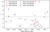 |
Fig. 4 Spectral index variation between observations in a given year as a function of mean spectral index. Red and blue markers represent thermal and non-thermal sources respectively. The horizontal dashed line represents the chosen variability threshold. |
4.3 Mass-loss rates and clumping ratios
In principle, one can estimate the mass-loss rates of our thermal radio stars using the prescriptions of Wright & Barlow (1975). Their model assumes a spherically symmetric wind, that only emits free-free emission. However, it is known that wind clumping can affect mass-loss rate estimates by factors of 3–4 (Smith 2014; Björklund et al. 2023). Therefore, for our thermal radio stars (α > 0), we computed the intrinsic mass-loss rates combined with the clumping factor (fcl ≡ ⟨ρ2⟩/⟨ρ⟩2) with the following expression (as in e.g. Andrews et al. 2019):
![Mathematical equation: $\[\dot{M} \sqrt{f_{\mathrm{cl}}^{[\text {band] }}}=0.095 \times \frac{\mu ~v_{\infty} ~S_{\nu}^{3 / 4} ~d^{3 / 2}}{Z\left(\gamma ~g_{\nu} ~\nu\right)^{1 / 2}}\left[M_{\odot} ~\mathrm{yr}^{-1}\right],\]$](/articles/aa/full_html/2024/12/aa51771-24/aa51771-24-eq27.png) (6)
(6)
with the free-free Gaunt factor gv defined as:
![Mathematical equation: $\[g_{\nu}=9.77\left(1+0.13 \log \left(\frac{T_{e}^{3 / 2}}{Z \nu}\right)\right),\]$](/articles/aa/full_html/2024/12/aa51771-24/aa51771-24-eq35.png) (7)
(7)
where μ is the mean molecular weight per ion, v∞ is the terminal wind velocity in units of km s−1 (both taken from Martins et al. 2008), Sν is the flux density in Janskys at the observing frequency ν in Hz, d represents the distance to the target in kpc units (we assume a distance of 8 kpc to the GC), Z is the ratio of electron to ion density, γ is the mean number of electrons per ion (both taken to be 1.0, as assumed in the Wolf-Rayet and O-type population of Andrews et al. 2019), and finally Te, the electron temperature, is assumed to be 104 K. Mass-loss rate uncertainties were calculated following the standard error propagation, ignoring the uncertainty related to the distance to the GC, for it systematically affects all cluster members in the same manner:
![Mathematical equation: $\[\begin{aligned}\frac{\sigma_M}{M_{\odot} ~\mathrm{yr}}= & \frac{\dot{M}}{M_{\odot} ~\mathrm{yr}}\left[\left(\frac{\sigma_{v_{\infty}}}{v_{\infty}}\right)^2+\left(\frac{\sigma_\mu}{\mu}\right)^2+\frac{9}{16}\left(\frac{\sigma_{S_\nu}}{S_\nu}\right)^2\right. \\& \left.+\left(\frac{\sigma_Z}{Z}\right)^2+\frac{1}{4}\left(\frac{\sigma_\gamma}{\gamma}\right)^2+\frac{1}{4}\left(\frac{\sigma_{g_\nu}}{g_\nu}\right)^2\right]^{1 / 2}.\end{aligned}\]$](/articles/aa/full_html/2024/12/aa51771-24/aa51771-24-eq36.png) (8)
(8)
We assumed 0.08 dex uncertainties for γ, Z, and μ, and a 10% relative error for the Gaunt factor as in Gallego-Calvente et al. (2021).
We used the combined X-band data from 2016 and 2022, given that none of these sources showcased significant variability on timescales of months, and because the combined images provide smaller flux uncertainties.
In addition, we also used the old VLA K-band data (central frequency of 22.5 GHz) from Lang et al. (2005) and computed the associated ![Mathematical equation: $\[\dot{M} \sqrt{f_{\mathrm{cl}}^{K}}\]$](/articles/aa/full_html/2024/12/aa51771-24/aa51771-24-eq37.png) values with Eq. (6). K-band fluxes are useful because they trace radio emission closer to the stellar atmosphere, and because non-thermal emission is less prominent at higher frequencies (Contreras et al. 1996), allowing us to establish an upper limit for the
values with Eq. (6). K-band fluxes are useful because they trace radio emission closer to the stellar atmosphere, and because non-thermal emission is less prominent at higher frequencies (Contreras et al. 1996), allowing us to establish an upper limit for the ![Mathematical equation: $\[\dot{M} \sqrt{f_{\mathrm{cl}}^{K}}\]$](/articles/aa/full_html/2024/12/aa51771-24/aa51771-24-eq38.png) value of F6. Table 3 shows the
value of F6. Table 3 shows the ![Mathematical equation: $\[\dot{M} \sqrt{f_{\mathrm{cl}}^{[\text {band] }}}\]$](/articles/aa/full_html/2024/12/aa51771-24/aa51771-24-eq39.png) factor derived for our thermal radio stars in both bands and the three different years.
factor derived for our thermal radio stars in both bands and the three different years.
Once the clumped mass-loss rates are associated with our thermal sources, we can gain some basic insight into their wind geometry by computing the clumping ratios ![Mathematical equation: $\[f_{\mathrm{cl}}^{\nu_{2}} / f_{\mathrm{cl}}^{\nu_{1}}\]$](/articles/aa/full_html/2024/12/aa51771-24/aa51771-24-eq40.png) , which follow from Eq. (6):
, which follow from Eq. (6):
![Mathematical equation: $\[\frac{f_{\mathrm{cl}}^{\nu_{2}}}{f_{\mathrm{cl}}^{\nu_{1}}}=\frac{g_{\nu_{1}}}{g_{\nu_{2}}} \frac{\nu_{1}}{\nu_{2}}\left(\frac{S_{\nu_{2}}}{S_{\nu_{1}}}\right)^{3 / 2} \text{where} ~\nu_{1}>\nu_{2}\]$](/articles/aa/full_html/2024/12/aa51771-24/aa51771-24-eq41.png) (9)
(9)
Again, we also used K-band fluxes from Lang et al. (2005) in Eq. (9) to better sample the radio-photosphere at different distances from the stellar surface. Table 4 shows the clumping ratios derived for our thermal sources.
We can see from the first two columns of Table 4 that, for most of our sources, clumping affects C- and X-bands similarly, while it may become more prevalent at K-band, which traces emission closer to the stellar surface. More multi-wavelength radio observations at higher frequencies (such as K-band) combined with infrared and submillimetre studies (carried out with instruments such as ALMA) may reveal a clearer picture of the radial dependence of clumping on observing frequency and thus help to establish stronger observational constraints on the intrinsic mass-loss of massive stars.
Although the clumping-scaled mass-loss rates broadly agree with existing literature (e.g. Vink 2022, Table 1), in this work we decided to refrain from making a detailed comparison between our results and current stellar evolutionary models, as it would be severely affected by uncertainties in extinction and clumping.
Differential extinction has been shown to be present throughout the GC (Schödel et al. 2010; Nogueras-Lara et al. 2021). Recent studies in the Arches field (Hosek et al. 2019) suggest lower mean extinction values (AKs ~ 2.4) than those provided by Figer et al. (2002), (AKs ~ 3.1) and Martins et al. (2008) (AKs ~ 2.8). Furthermore, recent quantitative spectroscopy of individual stars confirms the presence of differential extinction in the Arches and identifies large uncertainties in the resulting AKs depending on the adopted extinction laws, leading to up to 0.6 dex differences in the stellar luminosities (0.45 dex in mass-loss; Clark et al. 2023, see their Table 2).
Furthermore, using the clumping values shown in Clark et al. (2023) would be an oversimplification, because clumping is expected to be less prominent further away from the stellar surface (as shown in Runacres & Owocki (2002) models and our clumping ratios). The structure and geometry of massive stellar wind clumps are topics of ongoing research (e.g. Rubio-Díez et al. 2022) and a detailed observational analysis would require a multi-frequency, multi-facility study, which is left for future work and is beyond the scope of the present study.
![Mathematical equation: $\[\dot{M}^{[\mathrm{YY}]} \sqrt{f_{\mathrm{cl}}^{[\text {band] }}}\]$](/articles/aa/full_html/2024/12/aa51771-24/aa51771-24-eq28.png) factors for our sources.
factors for our sources.
Clumping ratios.
4.4 Nature of the sources
4.4.1 Colliding-wind binary candidates
We can distinguish between primary and secondary CWB candidates. To be placed in the former category, a given source must consistently present a negative or flat spectral index. However, significant flux variability could also be an indirect indicator of a particle-accelerating mechanism at work, as expected in colliding-wind regions (e.g. De Becker & Raucq 2013). Therefore, highly variable sources may be considered secondary candidates. Table 5 shows different parameters that may be used to discriminate CWBs among our radio detections.
In light of these results, we can confidently categorise F6, F19, F18, and F26 as primary CWB candidates due to their consistent α ≲ 0.0 values across the time span of our observations. Furthermore, F18 and F26 are clear examples of extreme variability (see Fig. 5) within months, which further strengthens their binary status. Moreover, the flux from F26 falls below the rms detection threshold (5.4 μJy/beam) for the 4 July observations in X-band. Such a drastic change in observed flux is not expected from the emission arising from the stellar winds of isolated stars.
As previously mentioned, some sources with α > 0 can still be considered secondary binary candidates. By looking at strong changes in flux (σVAR ≳ 10) over different observing epochs, we may categorise F7 and F9 as secondary CWB candidates. This hypothesis is further supported by the fact that these sources show clear X-ray counterparts detected by Chandra (Muno et al. 2009). Moreover, F7 has been identified as a long-period (P ≳ 1200 days) radial velocity binary candidate by Clark et al. (2023). Table 6 shows the properties of the Chandra counterparts to the radio detections.
It is possible that isolated massive stars produce thermal X-ray emission. Such emission can be caused by a difference in the velocity of two wind shocks travelling radially outwards from the stellar surface. However, the X-ray flux associated with such emission is estimated to be more than an order of magnitude lower than that produced in the colliding-wind region of a binary system (De Becker 2007) and therefore not in the detection limit of current X-ray observatories, such as Chandra, at the distance of the GC.
Finally, F12, F14, and F55 also show negative spectral indices (or compatibility with a flat spectrum within the uncertainties) at some point during our observations. In particular, F14 seems to show a change in the main emission mechanism from non-thermal during 2018 to thermal during 2022 observations. This could be indicating a binary system with a long orbital period, with the colliding-wind region changing from optically thin to optically thick. However, due to their relatively faint flux, especially in C-band, which is more prone to contamination from extended emission, we categorise these sources as secondary CWB candidates. Further monitoring of the Arches members with high-sensitivity, high-resolution radio-interferometers, such as the VLA or the future SKA-MID, may fully uncover the nature of the emission associated with these radio stars.
In all, out of the 23 radio stars we detect, we infer a binarity fraction of 9/23 ≈ 39% with radio data alone, which increases to 14/23 ≈ 61% if we take into account the radial velocity candidates from Clark et al. (2023). Furthermore, when we compare our candidates to those of Clark et al. (2023), we see that, with radio observations, we are able to discriminate two binary candidates – F19 and F26 – that did not meet the significance threshold of the radial velocity difference in their work, and we can add another candidate, F55, not present in their analysis.
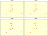 |
Fig. 5 Zoom onto the Arches cluster X-band images from 2016 (top) and 2022 (bottom). The blue and red circles show the positions of F18 and F26, respectively. |
Variability parameters.
Hardness ratios of the sources detected by Chandra.
4.4.2 Thermal radio stars
We can clearly categorise F3, Dong19, F5, F8, Dong96, and B1 as thermal sources whose emission is dominated by free-free emission from their stellar winds based on their consistently positive spectral indices and relatively low variability. However, it is still possible that the strong, optically thick winds of these Wolf-Rayet stars eclipse a potential non-thermal contribution from the colliding-wind region of a multiple system, especially in short-period binaries (De Becker 2007).
4.4.3 Ambiguous cases and other radio sources
The radio stars F1 and F2 show thermal spectral indices for most of the observations. However, in the case of F1, the X-band observations carried out on 11 April 2018 return a negative spectral index value (albeit with considerable uncertainties) and the 4 July 2022 observations show a considerably lower spectral index than the canonically thermal value of α ≈ 0.6, which may indicate a possible non-thermal component. Similar results are obtained for F2. The fact that this is a short-period (P ~ 10 day) binary with a low eccentricity (e = 0.075) orbit (Lohr et al. 2018) may explain why we do not detect clear traces of synchrotron emission in our observations with the exception of those carried out during 7 May 2022, whose spectral index is compatible with a flat spectrum – although uncertainties are large. Therefore, we cannot confidently classify these sources as CWB candidates with these results. In order to more reliably identify the nature of these radio stars, further ‘simultaneous’ multi-band observations are needed, which would result in more accurate computations of their spectral indices (we note that the spectral indices derived from the 4 July 2022 C- and X-band combined data have the lowest overall uncertainties in Table 1). Finally, despite showing significant variability, we categorise F4 as a thermal emitter given that its spectral index is consistently thermal in all our observations. A plausible explanation for F4 variability could be a large over-density in the winds in the radioemitting region. We deem it unlikely that F4 has undergone an eruptive mass-loss episode given its current evolutionary status, as these eruptive events are expected from luminous blue variables (e.g. Jiang et al. 2018), but not in WNh stars.
The rest of the detections not mentioned in the above subsections are too faint to be subject to the least-squared fitting from Sect. 3.4 or are not detected in a particular band, namely F16, F10, F15, F17, AR19, F28, and AR20. Most of them are 5σ detections in combined images or in the deep images. Given that they are mostly detected in X-band, we assumed thermal emission and included most of them in the mass-loss analysis (see Table 3). Furthermore, AR19 and AR20 are only detected in the X-band deep image, and they present no clear NIR stellar counterpart. For these reasons, they are excluded from the analysis presented in this work. In addition, some slightly extended sources near the cluster core can be seen in Fig. 1. As explained in Sect. 2, these sources are most likely remnants of the extended emission that were not fully removed by the u-v cut, as they do not present NIR stellar counterparts in the Hosek et al. (2022) catalogue, and do not match the synthesised beam shape in any image. Further observations carried out with different array configurations may help to better characterise this emission.
In the future, we will explore the full field of view of the observations and the properties of the non-stellar sources lying within the VLA primary beam.
5 Summary and conclusions
We present the most complete radio star catalogue (total of 23 radio stars) and the deepest (rms noise of ~2.5 μJy/beam in the case of X-band deep image) radio continuum C- and X-band images of the Arches cluster to date. With observations scattered across six years, the VLA sensitivity and angular resolution have allowed us to considerably improve our understanding of radio stars within the Arches cluster.
We find that around 60% of the radio stars in the Arches show significant flux variability on timescales of years. Furthermore, non-thermal sources are more likely to show drastic changes in flux densities on timescales of months.
We have also derived the clumping-scaled mass-loss rates of our thermal sources. These rates show values that are consistent with the existing literature. In addition, we provide a list of clumping ratios for our thermal sources. In general, according to the clumping ratios, the C- and X-band are similarly affected by clumping (ratios close to unity), but it may become more prominent at higher frequencies.
We classify four of our sources (F6, F18, F19, and F26) as CWBs, as they display α ≲ 0.0 across our observations. In addition, we show preliminary evidence that high radio-flux and/or spectral index variability may be an indirect indicator of multiplicity, an hypothesis that is strengthened by multi-wavelength counterparts to our radio detections (NIR radial velocity studies and X-ray point-sources). Therefore, we categorise F7, F9, F12, F14, and F55 as secondary CWB candidates, expanding the number of CWB candidates by four (F26 as a primary candidate and F7, F14, and F55 as secondary candidates) when compared to our pilot study (Gallego-Calvente et al. 2021). Most of the remaining radio stars for which spectral indices could be derived (12/18) show α ~ 0.6, which is consistent with thermal emission being the dominant mechanism at work. Thus, combining our CWB candidates with those from the radial velocity study of Clark et al. (2023), we find that 14/23 ≈ 61% of the radio stars of the Arches cluster are binary (or higher-order multiples) candidates.
We show preliminary evidence of spectral index variation in both thermal and non-thermal radio stars. Significant changes in α in the case of thermal emitters may be an indicator of changes in the clumping structure of their stellar winds or (more unlikely) eruptive episodes of mass-loss. Observed changes of flux and/or spectral index in non-thermal sources may be related to the orbital phases of binaries, but currently the data are still too incomplete for a conclusive study. Therefore, we emphasise the need for more surveys with more frequent, long-term sampling and simultaneous multi-band observations to disentangle the thermal and non-thermal contributions to the emission of a CWB candidate, which will help constrain the multiplicity of massive stars in regions of the parameter space not available for radial velocity studies.
Moreover, further simultaneous multi-wavelength observations may help to sample wind clumping at different atmospheric heights. Near-infrared, millimetre, and submillimetre radio observations, as well as centimetre radio continuum studies, could provide unprecedentedly detailed information on the clumping of massive stellar winds and thus improve our understanding of mass-loss and its effect on the poorly understood evolution of post main-sequence massive stars.
This study demonstrates the viability of using radio observations to discern thermal and non-thermal emission mechanisms of radio stars at the GC. Further monitoring, covering a dense temporal baseline, could help unravel the relationship between the dominant emission mechanism and the orbital phase of a multiple system, establishing radio continuum observations as a reliable and complementary method for studying the multiplicity fraction of young massive clusters.
Acknowledgements
We thank the NRAO staff for their help setting up the observations and their excellent guidance with the VLA pipeline and calibration process. Authors M.C.G., R.S., A.A., J.M., M.P.T., and A.T.G.C. acknowledge financial support from the Severo Ochoa grant CEX2021-001131-S funded by MCIN/AEI/10.13039/501100011033. M.G.C. and R.S. acknowledge support from grant EUR2022-134031 funded by MCIN/AEI/10.13039/501100011033 and by the European Union NextGenerationEU/PRTR. and by grant PID2022-136640NB-C21 funded by MCIN/AEI 10.13039/501100011033 and by the European Union. A.A. and M.P.T. acknowledge support from the Spanish National grant PID2020-117404GB-C21, funded by MCIN/AEI/10.13039/501100011033. A.T.G.C. acknowledges the Astrophysics and High Energy Physics programme supported by MCIN with funding from European Union NextGenerationEU (PRTR-C17.I1) and by Generalitat Valenciana. F.N., acknowledges support by grants PID2019-105552RB-C41 and PID2022-137779OB-C41 funded by MCIN/AEI/10.13039/501100011033 by “ERDF A way of making Europe”. Authors M.C.G., R.S. and J.M. acknowledge the Spanish Prototype of an SRC (SPSRC) service and support funded by the Ministerio de Ciencia, Innovación y Universidades (MICIU), by the Junta de Andalucía, by the European Regional Development Funds (ERDF) and by the European Union NextGenerationEU/PRTR. The SPSRC acknowledges financial support from the Agencia Estatal de Investigación (AEI) through the “Center of Excellence Severo Ochoa” award to the Instituto de Astrofísica de Andalucía (IAA-CSIC) (SEV-2017-0709) and from the grant CEX2021-001131-S funded by MICIU/AEI/10.13039/501100011033. J.M. acknowledges financial support from the grant PID2021-123930OB-C21 funded by MICIU/AEI/10.13039/501100011033 and by ERDF/EU.
Appendix A Additional material
Observations and image properties.
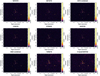 |
Fig. A.1 All images of the Arches cluster. |
Arches radio sources
References
- Abbott, D. C. 1980, ApJ, 242, 1183 [NASA ADS] [CrossRef] [Google Scholar]
- Andrews, H., Fenech, D., Prinja, R. K., Clark, J. S., & Hindson, L. 2019, A&A, 632, A38 [NASA ADS] [CrossRef] [EDP Sciences] [Google Scholar]
- Björklund, R., Sundqvist, J. O., Singh, S. M., Puls, J., & Najarro, F. 2023, A&A, 676, A109 [NASA ADS] [CrossRef] [EDP Sciences] [Google Scholar]
- CASA Team, Bean, B., Bhatnagar, S., et al. 2022, PASP, 134, 114501 [NASA ADS] [CrossRef] [Google Scholar]
- Castor, J. I., Abbott, D. C., & Klein, R. I. 1975, ApJ, 195, 157 [Google Scholar]
- Clark, J. S., Lohr, M. E., Najarro, F., Dong, H., & Martins, F. 2018a, A&A, 617, A65 [NASA ADS] [CrossRef] [EDP Sciences] [Google Scholar]
- Clark, J. S., Lohr, M. E., Patrick, L. R., et al. 2018b, A&A, 618, A2 [NASA ADS] [CrossRef] [EDP Sciences] [Google Scholar]
- Clark, J. S., Lohr, M. E., Najarro, F., Patrick, L. R., & Ritchie, B. W. 2023, MNRAS, 521, 4473 [NASA ADS] [CrossRef] [Google Scholar]
- Clark, J. S., Patrick, L. R., Najarro, F., Evans, C. J., & Lohr, M. 2021, A&A, 649, A43 [NASA ADS] [CrossRef] [EDP Sciences] [Google Scholar]
- Condon, J. J. 1997, PASP, 109, 166 [NASA ADS] [CrossRef] [Google Scholar]
- Contreras, M. E., Rodriguez, L. F., Gomez, Y., & Velazquez, A. 1996, ApJ, 469, 329 [NASA ADS] [CrossRef] [Google Scholar]
- De Becker, M. 2007, A&A Rev., 14, 171 [CrossRef] [Google Scholar]
- De Becker, M., & Raucq, F. 2013, A&A, 558, A28 [NASA ADS] [CrossRef] [EDP Sciences] [Google Scholar]
- Dong, H., Wang, Q. D., Cotera, A., et al. 2011, MNRAS, 417, 114 [Google Scholar]
- Dougherty, S. M., Beasley, A. J., Claussen, M. J., Zauderer, B. A., & Bolingbroke, N. J. 2005, ApJ, 623, 447 [NASA ADS] [CrossRef] [Google Scholar]
- Figer, D. F., McLean, I. S., & Morris, M. 1999, ApJ, 514, 202 [Google Scholar]
- Figer, D. F., Najarro, F., Gilmore, D., et al. 2002, ApJ, 581, 258 [Google Scholar]
- Gallego-Calvente, A. T., Schödel, R., Alberdi, A., et al. 2021, A&A, 647, A110 [NASA ADS] [CrossRef] [EDP Sciences] [Google Scholar]
- GRAVITY Collaboration (Abuter, R., et al.) 2019, A&A, 625, L10 [NASA ADS] [CrossRef] [EDP Sciences] [Google Scholar]
- Henshaw, J. D., Barnes, A. T., Battersby, C., et al. 2023, ASP Conf. Ser., 534, 83 [NASA ADS] [Google Scholar]
- Heywood, I., Rammala, I., Camilo, F., et al. 2022, ApJ, 925, 165 [NASA ADS] [CrossRef] [Google Scholar]
- Högbom, J. A. 1974, A&AS, 15, 417 [Google Scholar]
- Hosek, Matthew W., J., Lu, J. R., Anderson, J., et al. 2019, ApJ, 870, 44 [NASA ADS] [CrossRef] [Google Scholar]
- Hosek, M. W., Do, T., Lu, J. R., et al. 2022, ApJ, 939, 68 [NASA ADS] [CrossRef] [Google Scholar]
- Jiang, Y.-F., Cantiello, M., Bildsten, L., et al. 2018, Nature, 561, 498 [NASA ADS] [CrossRef] [Google Scholar]
- Kruijssen, J. M. D., & Longmore, S. N. 2013, MNRAS, 435, 2598 [Google Scholar]
- Lang, C., Johnson, K., Goss, W., & Rodriguez, L. 2005, AJ, 130, 2185 [NASA ADS] [CrossRef] [Google Scholar]
- Liermann, A., Hamann, W. R., & Oskinova, L. M. 2012, A&A, 540, A14 [NASA ADS] [CrossRef] [EDP Sciences] [Google Scholar]
- Lohr, M. E., Clark, J. S., Najarro, F., et al. 2018, A&A, 617, A66 [NASA ADS] [CrossRef] [EDP Sciences] [Google Scholar]
- Lu, J. R., Do, T., Ghez, A. M., et al. 2013, ApJ, 764, 155 [NASA ADS] [CrossRef] [Google Scholar]
- Martins, F., Hillier, D. J., Paumard, T., et al. 2008, A&A, 478, 219 [NASA ADS] [CrossRef] [EDP Sciences] [Google Scholar]
- Muno, M. P., Bauer, F. E., Baganoff, F. K., et al. 2009, ApJS, 181, 110 [CrossRef] [Google Scholar]
- Najarro, F., Figer, D. F., Hillier, D. J., & Kudritzki, R. P. 2004, ApJ, 611, L105 [Google Scholar]
- Nishiyama, S., Nagata, T., Tamura, M., et al. 2008, ApJ, 680, 1174 [Google Scholar]
- Nogueras-Lara, F., Schödel, R., & Neumayer, N. 2021, A&A, 653, A133 [NASA ADS] [CrossRef] [EDP Sciences] [Google Scholar]
- Nogueras-Lara, F., Schödel, R., Neumayer, N., et al. 2020, A&A, 641, A141 [EDP Sciences] [Google Scholar]
- Perley, R. A., & Butler, B. J. 2017, ApJS, 230, 7 [NASA ADS] [CrossRef] [Google Scholar]
- Rubio-Díez, M. M., Sundqvist, J. O., Najarro, F., et al. 2022, A&A, 658, A61 [NASA ADS] [CrossRef] [EDP Sciences] [Google Scholar]
- Runacres, M. C., & Owocki, S. P. 2002, A&A, 381, 1015 [NASA ADS] [CrossRef] [EDP Sciences] [Google Scholar]
- Sanchez-Bermudez, J., Alberdi, A., Schödel, R., et al. 2019, A&A, 624, A55 [EDP Sciences] [Google Scholar]
- Schödel, R., Najarro, F., Muzic, K., & Eckart, A. 2010, A&A, 511, A18 [Google Scholar]
- Smith, N. 2014, ARA&A, 52, 487 [NASA ADS] [CrossRef] [Google Scholar]
- Thompson, A. R., Moran, J. M., & Swenson, George W., J. 2017, Interferometry and Synthesis in Radio Astronomy, 3rd edn. (Berlin: Springer) [Google Scholar]
- Toalá, J. A., Todt, H., & Sander, A. A. C. 2024, MNRAS, 531, 2422 [CrossRef] [Google Scholar]
- Vink, J. S. 2022, ARA&A, 60, 203 [NASA ADS] [CrossRef] [Google Scholar]
- von Fellenberg, S. D., Gillessen, S., Stadler, J., et al. 2022, ApJ, 932, L6 [NASA ADS] [CrossRef] [Google Scholar]
- Wright, A. E., & Barlow, M. J. 1975, MNRAS, 170, 41 [Google Scholar]
- Zhao, J.-H., Morris, M. R., & Goss, W. M. 2020, ApJ, 905, 173 [NASA ADS] [CrossRef] [Google Scholar]
All Tables
All Figures
|
Fig. 1 Deep X-band image of the Arches cluster (see Table A.1 for details). Sources are labelled with the NIR stellar ID from Clark et al. (2018a) with the exception of the AR19 and AR20 sources (see Sect. 3.2). |
| In the text | |
|
Fig. 2 Flux versus frequency plot in logarithmic space in the case of the C-band observations from 10 June 2018. |
| In the text | |
|
Fig. 3 Positions of Dong19 and Dong96 with respect to the cluster core. |
| In the text | |
|
Fig. 4 Spectral index variation between observations in a given year as a function of mean spectral index. Red and blue markers represent thermal and non-thermal sources respectively. The horizontal dashed line represents the chosen variability threshold. |
| In the text | |
|
Fig. 5 Zoom onto the Arches cluster X-band images from 2016 (top) and 2022 (bottom). The blue and red circles show the positions of F18 and F26, respectively. |
| In the text | |
|
Fig. A.1 All images of the Arches cluster. |
| In the text | |
Current usage metrics show cumulative count of Article Views (full-text article views including HTML views, PDF and ePub downloads, according to the available data) and Abstracts Views on Vision4Press platform.
Data correspond to usage on the plateform after 2015. The current usage metrics is available 48-96 hours after online publication and is updated daily on week days.
Initial download of the metrics may take a while.