| Issue |
A&A
Volume 664, August 2022
|
|
|---|---|---|
| Article Number | A140 | |
| Number of page(s) | 12 | |
| Section | Interstellar and circumstellar matter | |
| DOI | https://doi.org/10.1051/0004-6361/202140914 | |
| Published online | 22 August 2022 | |
A multiwavelength study of the W33 Main ultracompact HII region
1
Indian Institute of Space Science and Technology (IIST),
Trivandrum
695 547, India
e-mail: skhan@mpifr-bonn.mpg.de
2
National Centre for Radio Astrophysics – Tata Institute of Fundamental Research,
Post Box 3,
Ganeshkhind PO,
Pune
411007, India
3
Max-Planck-Institut für Radioastronomie,
Auf dem Hügel 69,
53121
Bonn, Germany
4
IRAM,
300 rue de la piscine,
38406
Saint Martin d’Hères, France
Received:
28
March
2021
Accepted:
9
May
2022
Aims. The dynamics of ionized gas around the W33 Main ultracompact HII region is studied using observations of hydrogen radio recombination lines and a detailed multiwavelength characterization of the massive star-forming region W33 Main is performed.
Methods. We used the Giant Meterwave Radio Telescope (GMRT) to observe the H167α recombination line at 1.4 GHz at an angular resolution of 10″, and Karl. G. Jansky Very Large Array (VLA) data acquired in the GLOSTAR survey that stacks six recombination lines from 4–8 GHz at 25″ resolution to study the dynamics of ionized gas. We also observed the radio continuum at 1.4 GHz and 610 MHz with the GMRT and used GLOSTAR 4-8 GHz continuum data to characterize the nature of the radio emission. In addition, archival data from submillimeter to near-infrared wavelengths were used to study the dust emission and identify young stellar objects in the W33 Main star-forming region.
Results. The radio recombination lines were detected at good signal to noise in the GLOSTAR data, while the H167α radio recombination line was marginally detected with the GMRT. The spectral index of radio emission in the region determined from GMRT and GLOSTAR shows the emission to be thermal in the entire region. Along with W33 Main, an arc-shaped diffuse continuum source, G12.81–0.22, was detected with the GMRT data. The GLOSTAR recombination line data reveal a velocity gradient across W33 Main and G12.81–0.22. The electron temperature is found to be 6343 K and 4843 K in W33 Main and G12.81–0.22, respectively. The physical properties of the W33 Main molecular clump were derived by modeling the dust emission using data from the ATLASGAL and Hi-GAL surveys and they are consistent with the region being a relatively evolved site of massive star formation. The gas dynamics and physical properties of G12.81–0.22 are consistent with the HII region being in an evolved phase and its expansion on account of the pressure difference is slowing down.
Key words: stars: formation / HII regions / ISM: individual objects: W33 Main
© S. Khan et al. 2022
 Open Access article, published by EDP Sciences, under the terms of the Creative Commons Attribution License (https://creativecommons.org/licenses/by/4.0), which permits unrestricted use, distribution, and reproduction in any medium, provided the original work is properly cited.
This article is published in open access under the Subscribe-to-Open model. Subscribe to A&A to support open access publication.
1 Introduction
High-mass stars play an important role in the dynamics and evolution of the interstellar medium and the Galaxy. Along with supplying a large amount of ultraviolet (UV) photons to their surroundings, they also provide a feedback mechanism for the formation of the next generation of stars in a sequential manner (Elmegreen & Lada 1977; Lada 1987). The UV photons ionize the surrounding interstellar medium leading to the creation of HII regions. The HII regions may retain significant quantities of dust which can absorb an average of 34% of the UV photons (Binder & Povich 2018), re-emitting them at infrared wavelengths. While a massive star initially creates a hypercompact HII region with a typical size ≲ 0.05 pc, which expands to an ultracompact HII region with a size ≲0.1 pc, the Uv radiation from multiple massive stars may lead to the formation of a classical HII region complex in which the individual HII regions overlap with one another. These regions are bright at radio frequencies due to thermal bremsstrahlung emission. The study of these regions at radio wavelengths gives insight into the properties of the ionized gas. The physical conditions and the dynamics in HII regions can be probed by studying their emitted radio recombination lines (RRLs). In contrast, studies of HII regions at near-infrared wavelengths provide insight on the central stellar population, in particular on the massive young stellar objects (YSOs) they harbor. Thus, a multiwavelength study of HII regions can provide a comprehensive picture of the star formation activity in a massive star-forming region and their surroundings.
W33 is a massive star-forming region consisting of many HII regions, OB stars, and massive dust clumps in different evolutionary stages (Immer et al. 2014). Stier et al. (1984) conducted multi-band far-infrared (20–250 observations of the W33 complex and detected four distinct far-infrared sources in the complex, namely W33 Main, W33 A, W33 B, and W33 B1. Dust emission at 870 µm (ATLASGAL; Schuller et al. 2009) from the W33 complex reveals three large complexes – W33 A, W33 B, and W33 Main – along with several smaller clouds such as W33 A1, W33 B1, W33 Main1, among others. In this paper, we study the W33 Main region which hosts the brightest radio source in the W33 star-forming complex. The trigonometric parallactic distance to W33 determined from water masers is  kpc, which suggests an assignation to the Scutum spiral arm (Immer et al. 2013). The total bolometric luminosity and mass of the W33 complex are 5.5 – 105 L⊙ and 1.02 × 10⁴ M⊙, respectively (Immer et al. 2014).
W33 Main was found to have an enhanced ratio of the CO (32) to (1−0) line flux (R3−2/1−0 > 1.0; Kohno et al. 2018). This was interpreted as an indicator of the presence of massive stars since outflows and the strong radiation from massive stars heat the surrounding molecular clouds, resulting in a high value of R3−2/1−0. Messineo et al. (2015) performed a near-infrared spectroscopic survey of bright stars in selected regions of W33, which led to the identification of 14 early-type stars (OB and Wolf-Rayet type) with ages consistent with ~2–4 Myr.
Observations of H2CO and recombination lines toward the W33 complex reveal the presence of two velocity components at 35 km s−1 and 60 km s−1 which are associated with W33 Main and W33 B, respectively (Goss et al. 1978; Bieging et al. 1978). Similarly, Kohno et al. (2018) studied the molecular cloud of W33 using different CO lines and detected three velocity components at 35 km s−1, 45 km s−1, and 58 km s−1. Based on morphological correspondence and the fact that their R3−2/1−0 was greater than one, both the 35 km s−1 and the 58 km s−1 components were suggested to be associated with W33. In contrast, the association of the 45 km s−1 component with W33 is still not clear. Immer et al. (2013) found that water masers in W33 A, W33 Main (velocity of 35 km s−1), and W33 B (velocity of 58 km s−1) have the same parallactic distance which suggests that all of their molecular clumps belong to the W33 massive star-forming complex. Liu et al. (2021) studied the large-scale environment around W33 using the rotational (1−0) transitions of 12CO, 13CO, and C18O from the Purple Mountain Observatory and find evidence for a hub-filament system, with W33 being located at the central hub. Dewangan et al. (2020) also suggest that the star formation activity in W33 is triggered by converging and colliding flows from two velocity components ~35 and 53 km s−1.
Immer et al. (2014) constructed spectral energy distributions (SEDs) of the different clumps using data from the MSX, Hi-GAL, and ATLASGAL surveys. The SEDs were fit using a two component model from which the temperature of the cold dust component, peak H2 column density, and clump mass were determined. The temperature of the cold dust was found to vary between 25.0 and 42.5 K, suggesting that the clumps are in different evolutionary stages.
In this paper, we report the results of high resolution observations of the RRL and radio continuum at 1400 and 610 MHz, respectively, using the Giant Metrewave Radio Telescope (GMRT; Swarup et al. 1991) and continuum and RRL data from the GLOSTAR survey (Brunthaler et al. 2021) toward W33 Main. Also, based on data taken at submillimeter to near-infrared wavelengths, we present an analysis of the emission from the cool dust and the YSOs.
2 Observations and data analysis
2.1 GMRT radio observations
The 1400 MHz observations were carried out with the GMRT on 2016 August 23. The observations covered the H167α radio recombination line that has a rest frequency of 1399.368 MHz. The phase center for all the GMRT observation was 18h 14m 13s.96 and −17°55′44″.87. The GSB backend was used with a bandwidth of 16 MHz that was split into 512 channels giving a velocity resolution of 6.7 km s−1. The radio sources 3C48 and 3C286 were used as flux and bandpass calibrators, while 1911–201 was used as the gain calibrator. The total observing time was 4.6 h with an on-source integration time of approximately 3 h. The 610 MHz observations were carried out on 2016 September 16 with the GSB configured to have a bandwidth of 32 MHz and 256 channels. The sources 3C48 and 3C286 were used as primary calibrators, while 1911–201 and 1743–038 were used as gain calibrators. The W33 Main position was observed with an integration time of 30 minutes. The primary beam of a GMRT antenna at 1400 MHz and 610 MHz are 24′ and 43′, respectively. The details of the observations are listed in Table 1.
The data were reduced using the Astronomical Imaging and Processing Software (AIPS). The flagging of bad data and radio frequency interference and subsequent calibration were done using standard procedures. The continuum map of the region was then produced by imaging the line-free channels. Since GMRT does not carry out Doppler tracking, the spectral line data were first aligned using the task CVEL. The spectral line was found to be very weak with the line strength comparable to the residual ripple in the passband following bandpass calibration. However, the wavelength of the ripple was much larger than expected line width of the recombination line. Hence, the continuum was subtracted in a small sub-band of 32 channels around the line using the task UVLSF. The continuum subtracted data were then cleaned using standard procedures. In order to improve the signal-to-noise ratio (S/N), the spectral line cube was imaged using a uν taper of 50 kλ and natural weighting. The spectral line cube was seen to have stripe artifacts due to bad data from certain baselines. These data were identified and removed using the tasks UVMOD and UVSUB. The final angular resolution of the spectral cube is 10″, while that of the 1400 and 610 MHz continuum maps are 4.1″ × 2.1″ and 8.3″ × 4.2″, respectively. The data were then self-calibrated in order to reduce the residual calibration errors and improve the S/N.
The amplitudes of the 1400 and 610 MHz data have to be corrected for the contribution of the Galactic plane to the system temperature, which is not accounted for in the calibration process due to the calibrators being located outside the Galactic plane (Roy & Pramesh Rao 2004). The amplitudes were hence scaled by a correction factor of (Tgal + Tsys)/Tsys, where Tsys is the system temperatures corresponding to the calibrators and Tgal is the contribution of the Galaxy, which was estimated using the 408 MHz map of Haslam et al. (1982) and a spectral index of −2.6, where the flux density is defined as Sν ∝ να. The correction factors at 1400 MHz and 610 MHz were found to be 1.26 and 2.65, respectively. The data were then corrected for the response of the primary beam. The final root mean square (rms) in the radio maps were 1.6, 0.91, and 5.6 mJy beam−1 for the spectral cube, 1400 MHz continuum, and 610 MHz continuum, respectively.
Detail of the GMRT observation.
2.2 The GLObal view on STAR Formation in the Milky Way (GLOSTAR) VLA data
GLOSTAR is a survey of the Galactic Plane from 4-8 GHz covering 145 square degrees from 358° ≤ l ≤ 60°, |b| ≤1°, and the Cygnus X region. The survey was carried out using the Karl G. Jansky Very Large Array (VLA) in the compact D configuration and the more extended B configuration. The data products from the survey include continuum emission from 4.2-5.2 GHz and 6.4−7.4 GHz in full polarization, the H2CO line at 4.83 GHz, methanol maser line at 6.7 GHz, and seven radio recombination lines of hydrogen. The full technical details and data reduction of the survey are described in Brunthaler et al. (2021).
We obtained the GLOSTAR VLA-D configuration continuum image and the recombination line data cube. The continuum emission image is at a reference frequency of 5.8 GHz and has been constructed from mosaic of images of several frequency bins between 4 and 8 GHz (Medina et al. 2019; Brunthaler et al. 2021; Dzib et al., in prep.). The D-configuration continuum images are restored with a circular beam of 18″. We use six radio recombination lines observed in the GLOSTAR survey (H98α, H99α, H110α, H112α, H113α, H114α), which are stacked in velocity in order to increase the S/N. The data were gridded and imaged at a spectral resolution of 5 km s−1 and all the line cubes were smoothed to a spatial resolution of 25″ before stacking. The full description of the data reduction and calibration of the RRLs is given in Brunthaler et al. (2021) and Rugel et al. (in prep.).
2.3 Analysis of far-infrared data
In order to examine the cool emission toward W33 Main, we used data from the ATLASGAL (Schuller et al. 2009) and Hi-GAL (Molinari et al. 2010) surveys. We modeled the dust emission by fitting the SED from 870 to 70 µm on a per pixel basis. Since the images at different wavelengths have different resolution, plate scales, and data units, we first processed the data to have uniform resolution, plate scales, and data units. This analysis was carried out using the Herschel Interactive Processing Environment (HIPE). The data unit was converted to Jy pixel−1 for all wavelengths using the task “Convertlmage-Unit” Next, the task “PhotometricConvolution” was used to project the data to a common grid with the resolution and plate scale of the 500 µm map since it has the poorest resolution of all bands. The premade kernel (Aniano et al. 2011) was used for projecting the Herschel data, while the Gaussian kernel was used for the ATLASGAL data. After photometric convolution, all maps have the same resolution of 37″ and a plate scale of 7″ pixel−1. The maps show emission from the source as well as foreground and background emission from the Milky Way. After subtracting a constant background, the emission from each pixel was modeled by a gray body as given in Eq. (1):
 (1)
(1)
where Sν is the flux density of each pixel, Iν,bkg is the estimated background, Ω is the solid angle of an individual pixel (7″ × 7″), Bν is the Planck blackbody function, Td is the dust temperature, and τν is the optical depth, which depends on the frequency as τν = τ0(ν/ν0)ß, where ν0 is a reference frequency (chosen to correspond to a wavelength of 500 and β is the dust emissivity. The SED fits were carried out using the “MPFIT” function of Python’s “PYSPECKIT” module keeping Td, τ0, and β as free parameters with β being constrained to vary between one and three.
2.4 Ancillary data
Our study was complemented with data at mid-infrared and near-infrared wavelengths. We used data from the Spitzer GLIMPSE survey (3.6−8 µm; Benjamin et al. 2003), the UKIDSS Galactic Plane survey (1.25−2.15 µm;Lucas et al. 2008), and 2MASS (1.25−2.15 µm;Skrutskie et al. 2006) to study the YSO population and the ionizing stars in the region.
3 Results and discussion
3.1 Radio continuum emission
The left and middle panels of Fig. 1 shows the radio continuum emission toward the W33 Main region at 1400 MHz and 600 MHz. The angular size of the radio emission region of W33 Main is 64.8″ × 55.4″ which corresponds to linear sizes of 0.75 pc × 0.63 pc, respectively, at a distance of 2.4 kpc. Along with W33 Main, we also detected an arc-shaped diffuse continuum source, G12.81−0.22, which is located in southeast direction from W33 Main. The detail of radio continuum emission from both the sources at the GMRT frequencies are listed in Table 2.
The radio continuum emission at 5.8 GHz with a resolution of 18″ as seen in the GLOSTAR survey is shown in Fig. 1. While there is good correspondence between the radio emission at 5.8 and 1.4 GHz, the latter shows several diffuse emission components which are not visible in the GLOSTAR VLA-D configuration continuum map. At the GLOSTAR reference frequency (5.8 GHz), details on radio continuum emission are listed in Table 2.
The GMRT is an excellent instrument to look for and study the extended emission around ultracompact HII regions given the high sensitivity to extended emission, with 7′ being the largest detectable structure at 1400 MHz which is equivalent to 4.9 pc at 2.4 kpc. In order to check for the presence of extended emission, we generated a radio continuum map of the region at a resolution of 40″ and determined the total radio flux. Other than the presence of the diffuse region G12.81−0.22 to the southwest of W33 Main, we did not find any evidence for extended emission around W33 Main.
3.2 Spectral index map
In order to investigate the nature of the radio continuum emission (thermal versus nonthermal), we examined the spectral index of the radio emission. A spectral index that is larger than −0.1 typically indicates thermal emission, while a value lower than −0.5 suggests that the emission is nonthermal. First, we constructed a spectral index map from the GMRT 610 and 1400 MHz observations. One of the problems encountered when creating spectral index maps from interferometer observations is that the uν coverage of the antennas is different for different frequencies, resulting in varying sensitivities in different angular scales. To minimize this effect, we created maps of the region at both frequencies using the same uν coverage. The uν coverage of the 610 MHz observation ranges from 0.13 kλ to 50 kλ, while that of the 1400 MHz observation ranges from 0.21 kλ to 121 kλ. We imaged the region using a common cell size, angular resolution (specified by the BMAJ and BMIN keywords), and a common uν range of 0.21 kλ to 50 kλ. After this process, the beam size of both maps were 8.54″ × 4.15″ and the plate scale was 1″ per pixel.
Since the process of self-calibration results in the loss of absolute astrometry, determining the spectral index from the maps above could lead to systematic errors due to a position offset between the two maps. To correct for the differential astro-metric errors, we determined the positions of point sources that are detected at both frequencies using the task JMFIT and determined the position offset between the two maps. The 1400 MHz map was then shifted using the task GEOM, after which it was confirmed that the point sources line up on both maps accurately. Finally, the spectral index map was created using the task COMB with OPCODE set to “SPIX” or pixels having a radio continuum above the 5σ level at both frequencies. The spectral index map determined from this procedure is shown in the left panel of Fig. 2, with the uncertainty being shown in the right panel.
Since the GLOSTAR survey provides radio continuum images at several frequency bins, we determined the spectral index by fitting the flux density as a function of frequency at each pixel. Figure 3 shows the fit toward the peak emission of W33 Main and G12.81−0.22, and the values for the spectral index are tabulated in Table 3.
The spectral index determined from both GMRT observations and the GLOSTAR survey suggest that the emission is thermal in both sources. Furthermore, at the GMRT wavelengths, the continuum emission in W33 Main has a spectral index close to 2, while that in G12.81−0.22 is close to −0.1. At the location of peak emission, the spectral index between 610 MHz and 1.4 GHz is found to be 1.6 ± 0.3 and -0.02 ± 0.5 for W33 Main and G12.81−0.22, respectively (Table 3). At the frequencies corresponding to the GLOSTAR survey, the spectral index is found to be 0.35 ± 0.04 and -0.17 ± 0.09 at the location of peak emission of W33 Main and G12.81−0.22, respectively (Medina et al., in prep.). The W33 Main region shows a positive spectral index over the whole frequency range, while G12.81 −0.22 has a negative spectral index. This shows that the optical depth of radio continuum emission from W33 Main is very high at 1.4 GHz, reducing to moderate values in the 4−8 GHz band, while the radio continuum from G12.81−0.22 is optically thin even at 610 MHz.
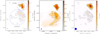 |
Fig. 1 Radio continuum map of source W33 Main and G12.81−0.20 at 1400 MHz (left panel) and 610 MHz (center panel) after primary beam correction and rescaling. The contour levels in the 1400 MHz map are at 3σ and factors of 3 thereafter. The contour levels in the 610 MHz map start at 3σ with a linear step size of 5σ thereafter, where σ is rms noise in the maps equivalent to 0.91 mJy beam−1 and 5.6 mJy beam−1 at 1400 and 610 MHz, respectively. Right panel: GLOSTAR wide-band reference frequency (5.8 GHz) map overlaid with the GMRT 1400 MHz contour. The blue-filled ellipse shows the corresponding beam size. |
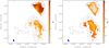 |
Fig. 2 Maps of the spectral index between the continuum emission at 610 MHz and 1400 MHz (left panel) and its uncertainty (right panel) of W33 Main and G12.81−0.22, overlaid with contours of the radio emission at 1400 MHz at full resolution. The contour levels are as described in Fig. 1 (left panel). The blue-filled ellipse shows the corresponding beam size. The blue cross corresponds to peak emission toward W33 Main and G12.81−0.22 at 1400 MHz. |
Summary of radio continuum emission toward W33 Main at different frequencies.
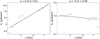 |
Fig. 3 Spectral index over 4−8 GHz from the GLOSTAR survey corresponding to peak emission toward W33 Main (left panel) and G12.81−0.22 (rightpanel; see also Medina et al., in prep.). |
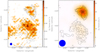 |
Fig. 4 Integrated line intensity map toward W33 Main and G12.81−0.22. Left panel: GMRT H167α at 10″ resolution. Right panel: GLOSTAR stacked recombination line at 25″ resolution, overlaid with contours of the radio emission at 1400 MHz at full resolution. The contour levels are as described in Fig. 1 (left panel). The blue-filled circle shows the corresponding beam size. |
Spectral index (α) of peak emission toward W33 Main and G12.81−0.22 between different frequency ranges.
3.3 Radio recombination lines
The GMRT observations included the low-frequency H167α recombination line, which can provide information on the diffuse ionized gas around W33 Main. The H167α line was marginally detected toward W33 Main and G12.81−0.22 at the 4.7σ and 4.4σ level, respectively. Since the emission was observed to be fragmented at the full resolution of the array, we restricted the resolution to 10″ for our analysis. The peak line strength toward W33 Main and G12.81−0.22 was 7.5 and 7.1 mJy beam−1, respectively, while the 1σ noise was 1.6 mJy beam−1. Figure shows the integrated intensity map of the H167α line. As expected, the line and the continuum emission are well correlated. Due to the poor S/N, the line profile could only be fitted at a few pixel locations. We are hence unable to trace the velocity field of ionized gas using the H167α line. The average line width of the H167α line was found to be 19.6 ± 7.5 and 18.1 ± 5.9 km s−1 toward W33 Main and G12.81−0.22, respectively. The line width in W33 Main is smaller than what is typically expected in compact HII regions.
The GLOSTAR survey provides recombination line data cubes by stacking six different recombination lines with a spectral resolution of 5 km s−1 and spatial resolution of 25″. The stacked recombination line was detected with a very good S/N and correlates well with the continuum emission at 1. and 5 GHz as shown in Fig.4. The peak line strength toward W33 Main and G12.81−0.22 was 680 and 83 mJy beam−1, respectively, while the 1σ noise in a line-free channel is 4.0 mJy beam−1. The average line width of the GLOSTAR stacked recombination line was found to be 36.3 ± 1.1 and 23.6 ± 1.4 km s−1 toward W33 Main and G12.81−0.22, respectively, which are comparable to typical line widths found in the compact and diffuse HII regions, respectively.
3.4 Electron temperature and photon hardening
The electron temperature can be determined using the radio continuum and recombination line data as long as the optical depth of the continuum emission is not very high. The methodology is described in Appendix A. As discussed in Sect. 3.2, while the radio continuum is optically thick in W33 Main at 1. GHz, the optical depth is moderate at the frequencies covered by the GLOSTAR survey.
Figure 5 shows the map of electron temperature in the region determined from the GLOSTAR survey. The average electron temperature toward W33 Main is found to be 6343 ± 222 K. This is consistent with earlier studies. Bieging et al. (1978) found an electron temperature of 6000 K, while Quireza et al. (2006) found an estimate of 7620 ± 100 K, with both studies using the H91α line, but at different angular resolutions. We are unable to determine the electron temperature at 1.4 GHz using the GMRT data toward the central regions of W33 Main due to the high optical depth of continuum emission. At the periphery of the HII region, where the optical depth is moderate, the electron temperature is measured to be 9145 ± 4710 K, where the large uncertainty is due to the poor S/N of the GMRT line data. Although the electron temperature cannot be determined from the recombination line when the radio continuum is optically thick, one can use the latter to obtain an estimate of the electron temperature. This is because the specific intensity of radio continuum emission is equal to the blackbody function of the electron temperature when the optical depth is very high, that is to say Iv = Bv(Te). Using this approach, we obtain an electron temperature of 10 000 to 12 100 K toward the central region of W33 Main. This is comparable to the results of Gardner et al. (1975), who derived the electron temperature toward peak emission to be between 10600 K to 12000 K using the H134α line. For the diffuse continuum source G12.81-0.22, the electron temperature is measured to be 4843 ± 355 K using GLOSTAR RRLs, and 6045 ± 2590 K using the GMRT observation of the H167α recombination line.
It can be seen that the electron temperature measured toward the central regions of W33 Main are significantly higher in GMRT compared to GLOSTAR. In contrast, the electron temperature measured toward G12.81−0.22 is broadly consistent at low and high frequencies. This is very likely due to the effects of photon hardening toward the boundary of HII regions (Wood & Mathis 2004). Since the bound-free absorption cross-section is lower at higher photon energy, the ionization at the edges of HII regions with a high optical depth is primarily driven by higher energy photons. Since the excess energy of the photons is converted into kinetic energy of the electrons, the electrons are expected to have a higher temperature. In the case of W33 Main, since the optical depth is high at 1.4 GHz, the continuum emission mainly originates from the outer edges of the HII region. Consequently, the electron temperature inferred from the radio continuum at 1.4 GHz is significantly higher than what is measured at GLOSTAR frequencies where the continuum optical depth is much lower. In G12.81−0.22, however, the optical depth of the radio continuum is low, even at 1.4 GHz, and the electron temperature measured using GMRT is found to be consistent with that of GLOSTAR. Even in G12.81−0.22, taking the center of the HII region to be the center of the arc, Fig. 5 shows that the electron temperature increases toward the outer regions, which may also be due to photon hardening. While noting that, Wilson et al. (2015) did not find evidence of photon hardening in Orion A and since the phenomenon of photon hardening is primarily discussed in the context of the warm diffuse interstellar medium of a galaxy, our observations suggest that it is detectable within individual HII regions as well.
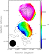 |
Fig. 5 Electron temperature map of W33 Main and G12.81−0.20 overlaid with contours of the radio emission at 1400 MHz at full resolution. The contour levels are as described in the left panel of Fig. 1. The black-filled circle represents the GLOSTAR beam size. |
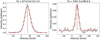 |
Fig. 6 Example of Gaussian fitted GLOSTAR stacked recombination line corresponding to the peak emission toward W33 Main (left panel) and G12.81−0.22 (right panel). Toward the peak emission of W33 Main, the line amplitude, line width, and velocity were found to be 622 ± 8.6 mJy beam−1, 39.3 ± 0.6 km s−1, and 36.7 ± 0.3 km s−1, respectively. For G12.81−0.22, toward the peak emission, the line amplitude, line width, and velocity were found to be 79.1 ± 2.9 mJy beam−1, 20.4 ± 0.9 km s−1 and 30.2 ± 0.4 km s−1, respectively. |
3.5 Gas dynamics
To investigate the dynamics of the ionized gas, we performed Gaussian fits to the GLOSTAR stacked recombination line data on a per pixel basis, with Fig. 6 showing sample fits toward the peak emission. The resulting maps of the velocity field and line width are shown in Fig. 7. The velocity field shows the presence of a velocity gradient in both the sources. In the case of W33 Main, the velocity increases from northeast to southwest with a velocity difference of around 10 km s−1. In the case of G12.81−0.22, there is a velocity gradient across the arc region in the radial direction, suggestive of expansion. The ratio of pressure in the HII region and the associated dust clump is given by the following:
 (2)
(2)
where 〈ne〉 and Te are the mean electron density and electron temperature of the HII regions, respectively (Tables 4 and 5); and 〈nD〉 and TD are the mean hydrogen density and dust temperature of the associated dust clump, respectively (see Sect. 3.7). For the HII regions toward W33 Main (regions 1, 2, and 3 as mentioned in Sect. 3.6), the ratio is 19, 13, and 20, respectively, which is ≫1. This suggests the ongoing pressure-driven expansion of HII regions. However, for G12.81−0.22, the ratio is close to unity, which indicates that the pressure-driven expansion for this HII region is coming to a halt.
Another interesting feature seen in the right panel of Fig. 7 is the presence of large line widths toward the northern region of W33 Main. W33 Main has an average electron temperature of 6360 K, which corresponds to a thermal line width of 17 km s−1. The northern region of W33 Main has a line width that is greater than 40 km s−1, which is significantly broader than the thermal broadening of the line. Following Keto et al. (2008), the recombination lines have a Voigt profile with a line width Δνv given by
![${\rm{\Delta }}{v_{\rm{V}}} = 0.5343{\rm{\Delta }}{v_{\rm{I}}} + {\left[ {{\rm{\Delta }}v_{\rm{G}}^2 + {{\left( {0.4657{\rm{\Delta }}{v_{\rm{I}}}} \right)}^2}} \right]^{1/2}},$](/articles/aa/full_html/2022/08/aa40914-21/aa40914-21-eq4.png) (3)
(3)
where ΔνI is the Lorentzian line width due to pressure broadening and ΔνG is the combination of thermal and dynamical broadening, given by
 (4)
(4)
Here, Δνt and Δνd refer to the thermal and dynamical broadening, respectively. The ratio of pressure and thermal broadening is given by (Brocklehurst & Seaton 1972),
 (5)
(5)
where n is transition number and ne is the electron density in cm−3. For the GLOSTAR survey, six recombination lines are observed, with the largest value of n being 114. The northern region of W33 Main has an electron density of 6.2 × 103 cm−3 (see Table 5), for which ΔνI/Δνt ≈ 0.23. Thus, the line width from pressure broadening is around 3.9 km s−1. Thus, from Eqs. (3) and (4), a line width in excess of 40 km s−1 implies dynamical broadening in excess of 30 km s−1. Balser et al. (2021) investigated the kinematic properties of Galactic HII regions using RRL emission and suggest that the HII regions with a center-peaked RRL width and velocity gradient favor solid-body rotation. In the case of W33 Main, by assuming the broad line width region to be the center, the velocity gradient structure suggests rotation motion. Balser et al. (2021) also report a velocity gradient for W33 Main. However, the spatial resolution of the GLOSTAR RRL map is increased compared to the observations used by Balser et al. (2021). Because of this, the velocity gradient does not appear to be homogeneous, but has a complex velocity structure. W33 Main consists of three HII regions (Anderson et al. 2014; see also Fig. 8 and Sect. 3.6), which have slightly different average velocities (Fig. 7). Also, the broad radio recombination lines are located toward the boundary of these HII regions. This indicates some complicated dynamic motions of the ionized gas inside W33 Main. For a detailed examination of the kinematics of the region, high-resolution molecular line observations are required.
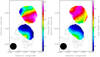 |
Fig. 7 Velocity field and a map of the line width obtained from the Gaussian fitting of GLOSTAR stacked recombination line data is shown in the left and right panels respectively. The maps are overlaid with contours of the radio emission at 1400 MHz at full resolution. The contour levels are as described in Fig. 1 (left panel). The black-filled circle represents the GLOSTAR beam size. |
3.6 Physical properties of the ionized gas
Anderson et al. (2014) made a catalog of over 8000 HII regions using data from the WISE satellite based on the morphology of mid-infrared emission. In the W33 Main region, four HII regions were identified (Table 4), of which three are toward W33 Main and one is toward the diffuse continuum source, G12.81−0.22 (see Fig. 8).
One can determine the physical properties of the HII regions using the electron temperature (Fig. 5) and the distance to the source; the results are tabulated in Table 5. The radii of the different regions are slightly different from that given by Anderson et al. (2014) to avoid overlap between the different regions and for better correlation between the infrared and radio emission. The peak emission measure can be estimated from the optical depth and electron temperature determined at the peak continuum emission using Eq. (A.4). The average electron density, Lyman continuum photon rate, and ionized mass are estimated using the equations given in Appendix B. Assuming that all the ionizing radiation comes from a single star, one can estimate the spectral type of the ionizing star using the Lyman continuum photon rate from Martins et al. (2005). Table 5 shows that the properties of W33 Main are consistent with it being an ultracompact HII region.
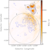 |
Fig. 8 GLIMPSE 8 µm map overlaid with blue contours of the radio emission at 1400 MHz at full resolution. The contour levels are as described in the left panel of Fig. 1. The black circles represent the HII regions toward W33 Main and G12.81−0.22 taken from the WISE catalog of Galactic HII regions (Anderson et al. 2014). Some regions have been slightly adjusted in order to avoid overlap and for better correlation with radio and 8 µm emission. |
HII regions in the W33 Main region from the WISE catalog of Galactic HII regions of Anderson et al. (2014).
Physical properties of regions.
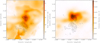 |
Fig. 9 Maps of the dust temperature (left panel) and H2 column density (right panel). The 1400 MHz radio continuum is overlaid as black contours with the contour levels as described in Fig. 1 (left panel). |
3.7 Emission from cold dust
Figure 9 shows the map of the dust temperature determined from the pixel-by-pixel fitting of the dust SED from 870 to 70 µm. We derived the column density of molecular hydrogen N(H2) from the dust optical depth at 500 µm using the following equation:
 (6)
(6)
where mH is the mass of the hydrogen atom, µ is the mean molecular weight, Kν is the dust opacity at 500 µm, and R is the gas-to-dust ratio. We have taken µ to be 2.8, assuming a hydrogen mass fraction of 0.7 (Kauffmann et al. 2008); the dust opacity at 500 µm to be 5.04 cm2 g−1, which is appropriate for dust grains with thin ice mantles (Ossenkopf & Henning 1994); and R to be 100. The right panel of Fig. 9 shows the distribution of the column density of molecular hydrogen in the region.
The peak dust temperature is seen to be ~45 K in the region. This is consistent with the dust temperature derived by Immer et al. (2014) who found a value of 42.5 ± 12.6 K. The dust temperature in the region is significantly higher than the mean kinetic temperature (based on NH3 observations) toward infrared dark clouds (14.8 K; Pillai et al. 2006) and 6.7 GHz methanol maser sites (26.0 K; Pandian et al. 2012). The high dust temperature can be inferred to reflect the more evolved state of the region. The peak column density of the clump in W33 Main is found to be 1.47 × 1023 cm−2 and the average column density in the region is 5.0 x 1022 cm−2. Immer et al. (2014) found the peak H2 column density (4.6 ± 1.6 × 1023 cm−2), which is higher than what is found in our study. However, this is in part due to them using the dust opacity from Hildebrand (1983), which is a factor of 2 smaller than that of Ossenkopf & Henning (1994) which have used in our study.
The total mass of the W33 Main molecular clump is estimated to be 4.6 × 10³ M⊙. This is consistent with the observation of Immer et al. (2014) who estimated the mass to be 4.0 ± 2.5 × 10³ M⊙. The mean hydrogen number density is found to be 4.7 × 104 cm−3, assuming an effective radius of 0.7 pc. The effective radius is obtained by Gaussian fitting of the clump and is given by reff = (θ1θ2/π)1/2, where θ1 and θ2 are the FWHM of the major and minor axes of the Gaussian, respectively. Kohno et al. (2018) used the C18O J = 1 − 0 observation to find the mass, number density, and mean hydrogen column density of W33 Main to be 9.5 × 10³ M⊙, 1.5 x 105 cm−3, and 5.1 × 1022 cm−2, respectively, which is roughly consistent with our value.
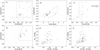 |
Fig. 10 Identification of YSOs using color-color criteria of (a) Allen et al. (2004), (b) Simon et al. (2007), (c) Gutermuth et al. (2008; Class I protostars), (d) Gutermuth et al. (2008; Class II YSOs), (e) Gutermuth et al. (2008) with NIR data from 2MASS, and (f) Gutermuth et al. (2008) with NIR data from UKIDSS. The cross, filled star, and filled triangles represent Class I, Class II, and Class I/II YSOs, respectively. |
3.8 Young stellar object population
The YSO population in the W33 Main region has been identified using the mid- and near-infrared colors. We first searched for point sources in the GLIMPSE, 2MASS, and UKIDSS (Galactic Plane Survey) catalogs within a 5′ region centered at (α, δ) = (18h 14m14s.6, −17°55−47″.5). We then constructed color–color diagrams (Fig. 10) and used the criteria mentioned in Allen et al. (2004), Simon et al. (2007), and Gutermuth et al. (2008) to identify and classify YSOs.
We used the criteria of Allen et al. (2004) in the [3.6]−[4.5] versus [5.8]−[8.0] color-color diagram (Fig. 10a) to identify ten Class I and three Class I/II YSOs in the region of interest. Simon et al. (2007) outlined criteria to identify YSOs based on the [3.6]−[4.5] versus [4.5]−[8.0] color-color diagram. This was used to identify 13 YSOs in the region (Fig. 10b). Gutermuth et al. (2008) used criteria on the [3.6]−[4.5] and [4.5]−[5.8] colors to identify Class I YSOs, and additional criteria based on [3.6]−[4.5] and [5.8]−[8.0] colors to detect Class II YSOs. Using these techniques, we identified 12 Class I and 11 Class II YSOs in the region (Figs. 10c and d). Using all four IRAC bands, we identified a total of 13 Class I, eight Class II, and four Class I/II YSOs.
The criteria above require photometry in all four IRAC bands for YSO identification. However, the GLIMPSE image shows the presence of significant extended emission at 8 µm in the vicinity of the radio continuum emission due to which photometry at 8 µm is often missing for sources that are detected in other IRAC bands. Hence, we used near-infrared photometry in J, H, and K bands from 2MASS and UKIDSS surveys and determined the intrinsic [K-[3.6]] and [3.6]−[4.5] colors following the method given in Gutermuth et al. (2008). While the 2MASS counterparts to the GLIMPSE point sources are provided in the GLIMPSE catalog, the UKIDSS counterparts were identified using a matching radius of 1.2″. The UKIDSS colors and magnitudes were then converted to the 2MASS photometric system using the transformations of Carpenter (2001), after which the intrinsic colors were calculated. Using 2MASS and UKIDSS photometry bands, we identified 11 Class I and eight Class II YSOs, and 21 Class I and 16 Class II YSOs, respectively. The number of YSOs detected using the UKIDSS band is larger than the 2MASS band due to the higher sensitivity of the UKIDSS survey. We detect a total of 25 Class I and 23 Class II sources in the region using this method after cross-matching (Figs. 10e and f).
Combining the various detection techniques, we have identified a total of 40 Class I, 29 Class II, and two Class I/II sources in the region. Figure 11 shows the distribution of identified YSOs on the map of the column density of molecular hydrogen. It is found that there is little correlation between the distribution of molecular gas and the distribution of YSOs, except for a small group of Class I YSOs to the west of W33 Main. This is mostly due to the significant extended emission associated with the HII region, which caused only very few point sources to be detected in the molecular clump. Moreover, the column density distribution of molecular hydrogen suggests that the extinction in the K band in the central region of W33 Main is as high as 7.5 magnitudes, which is equivalent to visual extinction of AV ≈67. The high extinction even in near- and mid-infrared wavelengths along with the presence of diffuse emission (Fig. 12) allow for a significant undetected YSO population in W33 Main. The YSO population is seen to correlate with the large-scale cloud structure well in the W33 region (Dewangan et al. 2020; Liu et al. 2021).
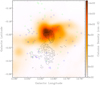 |
Fig. 11 Locations of Class I (blue cross), Class II (red cross) and Class I/II (magenta cross) YSOs overlaid on the hydrogen column density map with the 1400 MHz black contours. The contour levels are as described in Fig. 1 (left panel). |
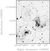 |
Fig. 12 Gray-scale UKIDSS K-band image of W33 Main. The black circles represent the HII region residing inside W33 Main. |
3.9 Nature of G12.81−0.22
The spectral index of radio emission in G12.81−0.22 shows that the emission is optically thin thermal emission. This together with the arc-like morphology of the source suggests that it traces part of an older HII region. The size and emission measure of G12.81 −0.22 (Table 5) also show it to be consistent with a compact HII region. The radial velocity gradient across the arc suggests that the HII region is expanding with a velocity ~6 km s−1. The Strömgren radius (Rst) of HII region is given by the following (Tielens 2005):
 (7)
(7)
where NLy is the Lyman continuum photon rate and  is the mean hydrogen density. Assuming that G12.81−0.22 had an initial hydrogen density that is characteristic of what is observed toward W33 Main at the present time, the Strömgren radius (Rst) of the region is 0.03 pc, which is much smaller than the current size of the HII region (~0.4 pc). This, together with the low continuum optical depth even at 610 MHz, shows that G12.81−0.22 is a much more evolved HII region and it is expanding on account of the pressure difference between the HII region and the ambient medium. Furthermore, this expansion is likely to be slowing down as mentioned in Sect. 3.5. Assuming expansion into a homogeneous molecular cloud, the dynamical age of the HII region was estimated using following equation (Wood & Churchwell 1989):
![${t_{{\rm{dyn}}}} = {4 \over 7}{{{R_{{\rm{st}}}}} \over {{c_{\rm{s}}}}}\left[ {{{\left( {{{{R_{\rm{f}}}} \over {{R_{{\rm{st}}}}}}} \right)}^{7/4}} - 1} \right],$](/articles/aa/full_html/2022/08/aa40914-21/aa40914-21-eq10.png) (8)
(8)
where Rf is the final radius of the HII region and cs is the isothermal sound speed. Taking the final radius as 0.4 pc and adopting a sound speed of 0.5 km s−1 (corresponding to a mean cold dust temperature of 35 K), we estimate the dynamical age of G12.81−0.22 to be 3.1 Myr. This is consistent with the stellar age ~2−4 Myr of the massive stars in the W33 massive star-forming region (Messineo et al. 2015).
4 Summary
We have carried out a multiwavelength study of the W33 Main region. High-resolution observations at 1400 and 610 MHz, using the GMRT and 4–8 GHz data from GLOSTAR, reveal the presence of two radio continuum sources in the region. The HII region associated with W33 Main is found to be moderately optically thick at 4–8 GHz and optically thick at 1.4 GHz, while the diffuse continuum source G12.81−0.22 is optically thin at all observed frequencies. Radio recombination lines are detected toward both continuum sources at a good S/N in GLOSTAR, while the H167α line was marginally detected by GMRT. The GLOSTAR recombination line data show the presence of a velocity gradient across W33 Main. Our work shows that the HII regions toward W33 Main are expanding and interacting with the surrounding material. The peak dust temperature in the region was found to be 45 K, which is consistent with W33 Main being a relatively evolved massive star-forming region. While a total of 71 YSOs were detected in the region, the presence of extended emission and high extinction at K band allows for the presence of a significant population of undetected YSOs that would be directly associated with the W33 Main molecular cloud. The physical properties of W33 Main reflect the evolved stage of the region and the properties of the diffuse continuum source, G12.81−0.22, the dynamics of ionized gas, and its dynamical age are consistent with the stellar age of the W33 complex.
Acknowledgements
We thank the staff of the GMRT that made these observations possible. GMRT is run by the National Center for Radio Astrophysics (NCRA) of the Tata Institute of Fundamental Research. DVL acknowledges the support of the Department of Atomic Energy, Government of India, under project no. 12-R&D-TFR-5.02−0700.
Appendix A Derivation of electron temperature
The detection of the recombination line allowed us to determine the electron temperature of the region using the line-to-continuum ratio using the following equations:
![${\tau _C} = - \ln \left[ {1 - {{{c^2}{I_C}} \over {2k{T_{\rm{e}}}{v^2}}}} \right]$](/articles/aa/full_html/2022/08/aa40914-21/aa40914-21-eq11.png) (A.1)
(A.1)
![${\tau _L} = - \ln \left[ {1 - {{{I_L}} \over {{I_C}}}\exp \left( {{\tau _C}} \right)\left( {1 - \exp \left( { - {\tau _C}} \right)} \right)} \right],$](/articles/aa/full_html/2022/08/aa40914-21/aa40914-21-eq12.png) (A.2)
(A.2)
where IC and IL refer to the specific intensity of the continuum and line, respectively, and τC and τL are the continuum and line optical depth, respectively. The optical depth τL corresponds to the center frequency of the line in terms of the emission measure given by the following (Wilson et al. 2009):
 (A.3)
(A.3)
where Δν is the line width. Under the Altenhoff approximation (Altenhoff et al. 1960), the continuum optical depth is given by
 (A.4)
(A.4)
When the radio continuum has a moderate optical depth, the electron temperature (Te) can thus be obtained from the ratio of line-to-continuum optical depth:
![${T_{\rm{e}}} = {\left[ {2.33 \times {{10}^4}{{\left( {{v \over {{\rm{GHz}}}}} \right)}^{2.1}}\left( {{{{\rm{kHz}}} \over {{\rm{\Delta }}v}}} \right){{{\tau _C}} \over {{\tau _L}}}} \right]^{1/1.15}}.$](/articles/aa/full_html/2022/08/aa40914-21/aa40914-21-eq15.png) (A.5)
(A.5)
When the radio continuum is optically thin, one can approximate τC/τL to be IC/IL in eq. (A.5) and it can estimate the electron temperature using the following equation (see, eg., Wenger et al. (2019)):
![$\left( {{{{T_{\rm{e}}}} \over {\rm{K}}}} \right) = {\left\{ {3.661 \times {{10}^4}{{{\rm{\Delta }}n} \over n}{f_{nm}}{{\left( {{v \over {{\rm{GHz}}}}} \right)}^{1.1}}\left( {{{{I_C}} \over {{I_L}}}} \right){{\left( {{{{\rm{\Delta }}\upsilon } \over {{\rm{km}}\,{{\rm{s}}^{ - 1}}}}} \right)}^{ - 1}}{{\left[ {1 + {{n\left( {^4{\rm{H}}{{\rm{e}}^ + }} \right)} \over {n\left( {{{\rm{H}}^ + }} \right)}}} \right]}^{ - 1}}} \right\}^{0.87}},$](/articles/aa/full_html/2022/08/aa40914-21/aa40914-21-eq16.png) (A.6)
(A.6)
where the expression fnm is the absorption oscillator strength and its approximation is given by (Menzel 1968)
 (A.7)
(A.7)
the expression (Δn/n fnm) = 0.19345 for Δn = 1 and n=107. After substitution, the final expression for the electron temperature is given by
![$\left( {{{{T_{\rm{e}}}} \over {\rm{K}}}} \right) = {\left\{ {7082.2{{\left( {{v \over {{\rm{GHz}}}}} \right)}^{1.1}}\left( {{{{I_C}} \over {{I_L}}}} \right){{\left( {{{{\rm{\Delta }}\upsilon } \over {{\rm{km}}\,{{\rm{s}}^{ - 1}}}}} \right)}^{ - 1}}{{\left[ {1 + {{n\left( {^4{\rm{H}}{{\rm{e}}^ + }} \right)} \over {n\left( {{{\rm{H}}^ + }} \right)}}} \right]}^{ - 1}}} \right\}^{0.87}},$](/articles/aa/full_html/2022/08/aa40914-21/aa40914-21-eq18.png) (A.8)
(A.8)
where Δν is the line width and n(4He+)/n(H+) is the ionic abundance ratio, which is considered to be a constant value of 0.07 ± 0.02 (Quireza et al. 2006).
When the optical depth was moderate, an iterative procedure was followed, wherein an initial guess for Te was provided to obtain the values of τC and τL from eqs. (A.1) and (A.2) after which a revised estimate of Te was obtained from eq. (A.5). The process was repeated until Te converged.
Appendix B Physical parameters of HII regions
The electron density and Lyman continuum flux rate at 5.8 GHz can be estimated using the equation given in Schmiedeke et al. (2016):
 (B.1)
(B.1)
 (B.2)
(B.2)
where θsource is the source size taken from the catalog of Anderson et al. (2014), Fv is the flux density at frequency ν, and D is the distance to the source.
Furthermore, the corresponding mass of ionized gas was estimated using the following equation (Tielens 2005):
 (B.3)
(B.3)
References
- Allen, L. E., Calvet, N., D’Alessio, P., et al. 2004, ApJS, 154, 363 [Google Scholar]
- Altenhoff, W., Mezger, P., Wendker, H., & Westerhout, G. 1960, Bonn, 59, 48 [NASA ADS] [Google Scholar]
- Anderson, L. D., Bania, T. M., Balser, D. S., et al. 2014, ApJS, 212, 1 [Google Scholar]
- Aniano, G., Draine, B. T., Gordon, K. D., & Sandstrom, K. 2011, PASP, 123, 1218 [Google Scholar]
- Balser, D. S., Wenger, T. V., Anderson, L. D., et al. 2021, ApJ, 921, 176 [NASA ADS] [CrossRef] [Google Scholar]
- Benjamin, R. A., Churchwell, E., Babler, B. L., et al. 2003, PASP, 115, 953 [Google Scholar]
- Bieging, J. H., Pankonin, V., & Smith, L. F. 1978, A&A, 64, 341 [NASA ADS] [Google Scholar]
- Binder, B. A., & Povich, M. S. 2018, ApJ, 864, 136 [CrossRef] [Google Scholar]
- Brocklehurst, M., & Seaton, M. J. 1972, MNRAS, 157, 179 [NASA ADS] [CrossRef] [Google Scholar]
- Brunthaler, A., Menten, K. M., Dzib, S. A., et al. 2021, A&A, 651, A85 [EDP Sciences] [Google Scholar]
- Carpenter, J. M. 2001, AJ, 121, 2851 [Google Scholar]
- Dewangan, L. K., Baug, T., & Ojha, D. K. 2020, MNRAS, 496, 1278 [NASA ADS] [CrossRef] [Google Scholar]
- Elmegreen, B. G., & Lada, C. J. 1977, ApJ, 214, 725 [Google Scholar]
- Gardner, F. F., Wilson, T. L., & Thomasson, P. 1975, Astrophys. Lett., 16, 29 [NASA ADS] [Google Scholar]
- Goss, W. M., Matthews, H. E., & Winnberg, A. 1978, A&A, 65, 307 [NASA ADS] [Google Scholar]
- Gutermuth, R. A., Myers, P., Megeath, S., et al. 2008, AJ, 674, 336 [NASA ADS] [CrossRef] [Google Scholar]
- Haslam, C. G. T., Salter, C. J., Stoffel, H., & Wilson, W. E. 1982, A&AS, 47, 1 [NASA ADS] [Google Scholar]
- Hildebrand, R. H. 1983, QJRAS, 24, 267 [NASA ADS] [Google Scholar]
- Immer, K., Reid, M. J., Menten, K. M., Brunthaler, A., & Dame, T. M. 2013, A&A, 553, A117 [NASA ADS] [CrossRef] [EDP Sciences] [Google Scholar]
- Immer, K., Galván-Madrid, R., König, C., Liu, H. B., & Menten, K. M. 2014, A&A, 572, A63 [NASA ADS] [CrossRef] [EDP Sciences] [Google Scholar]
- Kauffmann, J., Bertoldi, F., Bourke, T. L., Evans, N. J. I., & Lee, C. W. 2008, A&A, 487, 993 [NASA ADS] [CrossRef] [EDP Sciences] [Google Scholar]
- Keto, E., Zhang, Q., & Kurtz, S. 2008, ApJ, 672, 423 [NASA ADS] [CrossRef] [Google Scholar]
- Kohno, M., Torii, K., Tachihara, K., et al. 2018, PASJ, 70, S50 [Google Scholar]
- Lada, C. J. 1987, in IAU Symposium, Star Forming Regions, eds. M. Peimbert, & J. Jugaku, 115, 1 [NASA ADS] [Google Scholar]
- Liu, X.-L., Xu, J.-L., Wang, J.-J., et al. 2021, A&A, 646, A137 [NASA ADS] [CrossRef] [EDP Sciences] [Google Scholar]
- Lucas, P. W., Hoare, M. G., Longmore, A., et al. 2008, MNRAS, 391, 136 [Google Scholar]
- Martins, F., Schaerer, D., & Hillier, D. J. 2005, A&A, 436, 1049 [NASA ADS] [CrossRef] [EDP Sciences] [Google Scholar]
- Medina, S. N. X., Urquhart, J. S., Dzib, S. A., et al. 2019, A&A, 627, A175 [NASA ADS] [CrossRef] [EDP Sciences] [Google Scholar]
- Menzel, D. H. 1968, Nature, 218, 756 [CrossRef] [Google Scholar]
- Messineo, M., Clark, J. S., Figer, D. F., et al. 2015, ApJ, 805, 110 [Google Scholar]
- Molinari, S., Swinyard, B., Bally, J., et al. 2010, PASP, 122, 314 [Google Scholar]
- Ossenkopf, V., & Henning, T. 1994, A&A, 291, 943 [NASA ADS] [Google Scholar]
- Pandian, J. D., Wyrowski, F., & Menten, K. M. 2012, ApJ, 753, 50 [NASA ADS] [CrossRef] [Google Scholar]
- Pillai, T., Wyrowski, F., Carey, S. J., & Menten, K. M. 2006, A&A, 450, 569 [NASA ADS] [CrossRef] [EDP Sciences] [Google Scholar]
- Quireza, C., Rood, R. T., Bania, T. M., Balser, D. S., & Maciel, W. J. 2006, ApJ, 653, 1226 [Google Scholar]
- Roy, S., & Pramesh Rao, A. 2004, MNRAS, 349, L25 [NASA ADS] [CrossRef] [Google Scholar]
- Schmiedeke, A., Schilke, P., Möller, T., et al. 2016, A&A, 588, A143 [NASA ADS] [CrossRef] [EDP Sciences] [Google Scholar]
- Schuller, F., Menten, K. M., Contreras, Y., et al. 2009, A&A, 504, 415 [NASA ADS] [CrossRef] [EDP Sciences] [Google Scholar]
- Simon, J. D., Bolatto, A. D., Whitney, B. A., et al. 2007, ApJ, 669, 327 [NASA ADS] [CrossRef] [Google Scholar]
- Skrutskie, M. F., Cutri, R. M., Stiening, R., et al. 2006, AJ, 131, 1163 [NASA ADS] [CrossRef] [Google Scholar]
- Stier, M. T., Jaffe, D. T., Rengarajan, T. N., et al. 1984, ApJ, 283, 573 [NASA ADS] [CrossRef] [Google Scholar]
- Swarup, G., Ananthakrishnan, S., Kapahi, V. K., et al. 1991, Curr. Sci., 60, 95 [Google Scholar]
- Tielens, A. G. G. M. 2005, The Physics and Chemistry of the Interstellar Medium [Google Scholar]
- Wenger, T. V., Balser, D. S., Anderson, L. D., & Bania, T. M. 2019, ApJ, 887, 114 [NASA ADS] [CrossRef] [Google Scholar]
- Wilson, T. L., Rohlfs, K., & Hüttemeister, S. 2009, Tools of Radio Astronomy [Google Scholar]
- Wilson, T. L., Bania, T. M., & Balser, D. S. 2015, ApJ, 812, 45 [NASA ADS] [CrossRef] [Google Scholar]
- Wood, D. O. S., & Churchwell, E. 1989, ApJS, 69, 831 [Google Scholar]
- Wood, K., & Mathis, J. S. 2004, MNRAS, 353, 1126 [NASA ADS] [CrossRef] [Google Scholar]
All Tables
Spectral index (α) of peak emission toward W33 Main and G12.81−0.22 between different frequency ranges.
HII regions in the W33 Main region from the WISE catalog of Galactic HII regions of Anderson et al. (2014).
All Figures
|
Fig. 1 Radio continuum map of source W33 Main and G12.81−0.20 at 1400 MHz (left panel) and 610 MHz (center panel) after primary beam correction and rescaling. The contour levels in the 1400 MHz map are at 3σ and factors of 3 thereafter. The contour levels in the 610 MHz map start at 3σ with a linear step size of 5σ thereafter, where σ is rms noise in the maps equivalent to 0.91 mJy beam−1 and 5.6 mJy beam−1 at 1400 and 610 MHz, respectively. Right panel: GLOSTAR wide-band reference frequency (5.8 GHz) map overlaid with the GMRT 1400 MHz contour. The blue-filled ellipse shows the corresponding beam size. |
| In the text | |
|
Fig. 2 Maps of the spectral index between the continuum emission at 610 MHz and 1400 MHz (left panel) and its uncertainty (right panel) of W33 Main and G12.81−0.22, overlaid with contours of the radio emission at 1400 MHz at full resolution. The contour levels are as described in Fig. 1 (left panel). The blue-filled ellipse shows the corresponding beam size. The blue cross corresponds to peak emission toward W33 Main and G12.81−0.22 at 1400 MHz. |
| In the text | |
|
Fig. 3 Spectral index over 4−8 GHz from the GLOSTAR survey corresponding to peak emission toward W33 Main (left panel) and G12.81−0.22 (rightpanel; see also Medina et al., in prep.). |
| In the text | |
|
Fig. 4 Integrated line intensity map toward W33 Main and G12.81−0.22. Left panel: GMRT H167α at 10″ resolution. Right panel: GLOSTAR stacked recombination line at 25″ resolution, overlaid with contours of the radio emission at 1400 MHz at full resolution. The contour levels are as described in Fig. 1 (left panel). The blue-filled circle shows the corresponding beam size. |
| In the text | |
|
Fig. 5 Electron temperature map of W33 Main and G12.81−0.20 overlaid with contours of the radio emission at 1400 MHz at full resolution. The contour levels are as described in the left panel of Fig. 1. The black-filled circle represents the GLOSTAR beam size. |
| In the text | |
|
Fig. 6 Example of Gaussian fitted GLOSTAR stacked recombination line corresponding to the peak emission toward W33 Main (left panel) and G12.81−0.22 (right panel). Toward the peak emission of W33 Main, the line amplitude, line width, and velocity were found to be 622 ± 8.6 mJy beam−1, 39.3 ± 0.6 km s−1, and 36.7 ± 0.3 km s−1, respectively. For G12.81−0.22, toward the peak emission, the line amplitude, line width, and velocity were found to be 79.1 ± 2.9 mJy beam−1, 20.4 ± 0.9 km s−1 and 30.2 ± 0.4 km s−1, respectively. |
| In the text | |
|
Fig. 7 Velocity field and a map of the line width obtained from the Gaussian fitting of GLOSTAR stacked recombination line data is shown in the left and right panels respectively. The maps are overlaid with contours of the radio emission at 1400 MHz at full resolution. The contour levels are as described in Fig. 1 (left panel). The black-filled circle represents the GLOSTAR beam size. |
| In the text | |
|
Fig. 8 GLIMPSE 8 µm map overlaid with blue contours of the radio emission at 1400 MHz at full resolution. The contour levels are as described in the left panel of Fig. 1. The black circles represent the HII regions toward W33 Main and G12.81−0.22 taken from the WISE catalog of Galactic HII regions (Anderson et al. 2014). Some regions have been slightly adjusted in order to avoid overlap and for better correlation with radio and 8 µm emission. |
| In the text | |
|
Fig. 9 Maps of the dust temperature (left panel) and H2 column density (right panel). The 1400 MHz radio continuum is overlaid as black contours with the contour levels as described in Fig. 1 (left panel). |
| In the text | |
|
Fig. 10 Identification of YSOs using color-color criteria of (a) Allen et al. (2004), (b) Simon et al. (2007), (c) Gutermuth et al. (2008; Class I protostars), (d) Gutermuth et al. (2008; Class II YSOs), (e) Gutermuth et al. (2008) with NIR data from 2MASS, and (f) Gutermuth et al. (2008) with NIR data from UKIDSS. The cross, filled star, and filled triangles represent Class I, Class II, and Class I/II YSOs, respectively. |
| In the text | |
|
Fig. 11 Locations of Class I (blue cross), Class II (red cross) and Class I/II (magenta cross) YSOs overlaid on the hydrogen column density map with the 1400 MHz black contours. The contour levels are as described in Fig. 1 (left panel). |
| In the text | |
|
Fig. 12 Gray-scale UKIDSS K-band image of W33 Main. The black circles represent the HII region residing inside W33 Main. |
| In the text | |
Current usage metrics show cumulative count of Article Views (full-text article views including HTML views, PDF and ePub downloads, according to the available data) and Abstracts Views on Vision4Press platform.
Data correspond to usage on the plateform after 2015. The current usage metrics is available 48-96 hours after online publication and is updated daily on week days.
Initial download of the metrics may take a while.